Deep Transfer Learning for Modality Classification of Medical Images


1
School of Computer Science and Technology, Dalian University of Technology, Dalian 116024, China
2
School of Computer Science & Engineering, Dalian Minzu University, Dalian 116600, China
3
School of Software Engineering, Dalian University of Foreign Languages, Dalian 116044, China
*
Author to whom correspondence should be addressed.
Information 2017, 8(3), 91; https://doi.org/10.3390/info8030091
Submission received: 7 July 2017
/
Revised: 26 July 2017
/
Accepted: 27 July 2017
/
Published: 29 July 2017
Abstract
:Medical images are valuable for clinical diagnosis and decision making. Image modality is an important primary step, as it is capable of aiding clinicians to access required medical image in retrieval systems. Traditional methods of modality classification are dependent on the choice of hand-crafted features and demand a clear awareness of prior domain knowledge. The feature learning approach may detect efficiently visual characteristics of different modalities, but it is limited to the number of training datasets. To overcome the absence of labeled data, on the one hand, we take deep convolutional neural networks (VGGNet, ResNet) with different depths pre-trained on ImageNet, fix most of the earlier layers to reserve generic features of natural images, and only train their higher-level portion on ImageCLEF to learn domain-specific features of medical figures. Then, we train from scratch deep CNNs with only six weight layers to capture more domain-specific features. On the other hand, we employ two data augmentation methods to help CNNs to give the full scope to their potential characterizing image modality features. The final prediction is given by our voting system based on the outputs of three CNNs. After evaluating our proposed model on the subfigure classification task in ImageCLEF2015 and ImageCLEF2016, we obtain new, state-of-the-art results—76.87% in ImageCLEF2015 and 87.37% in ImageCLEF2016—which imply that CNNs, based on our proposed transfer learning methods and data augmentation skills, can identify more efficiently modalities of medical images.
1. Introduction
With the ease of Internet access, the size of the medical literature has grown exponentially over the past few years [1]. Medical images in articles provide basic knowledge in visualization of body parts, in their treatment, and in tracking disease, which makes the clinical care and diagnosis of diseases practicable [2,3,4]. Different sorts of medical image technologies provide an enormous amount of images with various medical modalities and other image types, such as Computerized Tomography, X-ray, or generic biomedical illustrations [5]. To aid the clinician and the researcher to retrieve required images, many tools have been developed to formulate and execute queries based on the visual content [6]. Content-based medical image retrieval systems, such as OPENi [7], could be improved by filtering our non-relevant image types using the modality information [6,8], but not all medical images are annotated appropriately.
To overcome the limited number of labeled images with reliable modality information, one way is to assign manually modalities to all medical images. However, this is both time consuming and costly. Another possibility is to perform automatic modality classification of the images using feature engineering methods [9,10,11,12,13,14] (see Section 2). The performance of these approaches is good but limited to the choice of “hand-crafted” features and a clear awareness of prior domain knowledge. Learning features from data has become popular both in academia and in industry, because many interesting priors can be conveniently captured by a learner [15].
Convolutional neural networks (CNNs) are designed to learn features from data that come in the form of multiple arrays, for example, a color image. They achieve many practical successes [16,17,18,19] (see Section 2) in ImageNet benchmark [20] and have recently been widely adopted by the computer vision community [21]. When large scale training datasets are available, CNNs are capable of learning more expressive representations of image data in general object recognition [20]. However, in real world applications (e.g., the medical images modality classification), it is expensive or impossible to re-collect the needed training data and train CNNs from scratch. CNNs may be hindered to disentangle the factors of variation by the limited samples with highly variable [22].
Transfer learning between task domains would be desirable. For the task of medical image classification, the training dataset is not large (thousands), therefore it is a good choice [23,24] to pre-train a CNN on a very large dataset (e.g., ImageNet, which contains 1.2 million natural images with 1000 categories), and then use the pre-trained CNN either as an initialization for further fine-tuning [25,26] or a fixed feature extractor [27] (see Section 2). Since the current medical dataset is small, it is likely best to only train a linear classifier rather than to fine-tune the pre-trained CNN due to overfitting concerns. Because the medical dataset is very different from the original natural dataset of ImageNet, another classifier needs to be trained from activations somewhere earlier [28] in the network. Features extracted from the top of the pre-trained network may be too dataset-specific and would not be able to distinguish medical images.
In this article, we first train from scratch a deep CNN without too many layers on medical data to capture domain-specific information. Then, we explore another transfer learning framework to capture both generic and domain-specific features. We reserve generic characteristics by fixing most layers of deeper CNNs pre-trained on ImageNet and learn new specific representations through replacing and retraining the classifier (top layers) on top of the pre-trained network on medical datasets. To address the greatest challenge that is the small scale of current dataset. We employ two methods of data augmentation to aid CNNs to reach their full potential and further improve modality classification performance. After evaluating our proposed model on the subfigure classification task in ImageCLEF2015 and ImageCLEF2016, we obtain better performance than the state of the art visual methods—76.87% in ImageCLEF2015 and 87.37% in ImageCLEF2016.
2. Related Work
Due to its importance in detecting modalities of medical images, a lot of research has been proposed for the task of modality classification, including feature engineering methods [9,10,11,12,13,14] and deep learning-based approaches [25,27]. Since deep learning-based methods do not need hand-crafted features, they have shown promising potential in dealing with modality classification task.
Over the years, various effective feature engineering techniques for medical image classification have been developed. De Herrera et al. [9] combine SIFT (Scale Invariant Feature Transform) [29] with BoC (Bag-of-Colors) [30] features to represent medical images. Pelka et al. [10,14] extract eight kinds of low-level features from images to train a multiclass linear SVM and a obtain state-of-the-art visual result (60.91%) in ImageCLEF2015. Koitka et al. [11] apply many state-of-the-art visual descriptors to describe an image with color, texture, and shape information. Valavanis [12] adopts various visual features, such as Bag-of-Visual-Words [31] and Quad-Tree [32] BoC (Bag-of-Colors). Li, P. et al. [13] also apply a hierarchical classifier using multiple visual descriptors. The performance of these approaches depends on the quality of features hand-crafted by domain experts. It is hard to capture a substantial number of possible input variations very well.
CNNs have led to a series of breakthroughs for image classification [16,17,18,19,20]. There are four key ideas [21] behind CNNs: local connections, shared weights, pooling, and the use of many layers. Different feature maps are responsible to detect local distinctive motifs. Sharing the same weights among units at different locations tend to detect the same pattern in different parts of the image. The role of the pooling layer is to merge semantically similar features into one, reduce the dimension of the representation, and create an invariance to small shifts and distortions. Recently, with the popularity of CNNs, deeper and deeper networks have been proposed, e.g., AlexNet [16], VGGNet [17], GoogLeNet [18], and ResNet [19]. The initial landmark breakthrough of Krizhevsky et al. [16] is achieved by their AlexNet CNN with eight weight layers. Simonyan et al. [17] propose VGGNet with 16 weight layers to investigate how the CNNs’ depth affects their accuracy in the large-scale image recognition setting. Szegedy et al. [18] introduce GoogLeNet architecture with more weight layers but much fewer parameters than AlexNet and VGGNet. He et al. [19] present deep residual networks (ResNet) with a depth of up to 152 weight layers, which address the degradation problem by introducing a deep residual learning framework. CNNs generally require a large-scale dataset to reach their full potential. It is difficult to acquire large, expertly labeled training datasets in consideration of the time and labor cost involved. Take ImageCLEF medical [5,33,34] as an example; it provides thousands of labeled medical images for modality classification, which is a much smaller amount than the ImageNet dataset [20], which contains 1.2 million natural images.
Our previous work [22] in ImageCLEF2013 is the first attempt to train from scratch multiple CNNs to learn features from medical images for describing their modalities, and it achieves a competitive result. Since deep CNNs take several weeks to train across multiple GPUs on ImageNet, it is common to see people release their final network checkpoints for the benefit of others who can use the networks as a fixed-feature extractor or for fine-tuning. Koitka et al. [12] extract visual features from the top of the pre-trained ResNet [19] to train another classifier to predict modality and achieve state-of-the-art performance (85.38%) in ImageCLEF2016. Kumar et al. [25] combine fine-tuned AlexNet [16] and GoogLeNet [18] to distinguish subtle differences between image modalities. Zhang et al. [26] use the synergic signal system to combine dual ResNets, which are pre-trained on large scale natural images and fine-tuned on medical figures. However, it is hard to capture nuances between modalities by fine-tuning CNNs with enormous parameters under the circumstance that there are not sufficient training samples.
The ImageCLEF dataset is small and very different from the ImageNet dataset. We keep some of earlier layers fixed (due to overfitting concerns) and only retrain the higher-level portion of the network. This is motivated by the observation that the earlier features of a CNN contain more generic features (e.g., edge detectors or color blob detectors) that may be useful to current task, but later layers of the CNN become progressively more specific to the details of the classes contained in the ImageNet dataset. To address the difficulty of learning from the imbalanced dataset with limited samples, other CNN-based methods for modality classification have expanded the training dataset [22,25,27].
3. Methods
This section describes the architecture of our proposed model including three types of deep convolutional neural networks (CNNs) with different depths and a different voting system (see Figure 1).
3.1. Convolutional Neural Networks
We first took two types of very deep CNNs (VGGNet-16 and ResNet-50, shown in Figure 1) with different depths that had been pretrained (initialised) on natural image dataset (ImageNet). Then we trained from scratch a “shallower” CNN (CNN-6) on the medical dataset. The softmax function is implemented at the final layer to output the prediction probabilities, to determine the class of the image.
We used the following different CNNs, with their own different capabilities, to explore the central importance of networks’ depth:
1. CNN-6
This CNN has only six weight layers similar to [22,35,36]. The first two convolutional layers contain 32 kernels of size 3 × 3, and the second two convolutional layers have 64 kernels of size 3 × 3. The second and fourth convolutional layers are interleaved with max pooling layers of dimension 2 × 2 with a dropout of 0.25. Then a full-connected layer with 512 neurons and a dropout of 0.5 is followed by a full-connected layer with 30 neurons. The ReLU activation function is applied to all four convolutional layers and the first full-connected layer. We use Glorot [37] uniform to initial weights and train the model from scratch.
2. VGGNet-16
This deeper CNN has a depth of 16 weight layers proposed by the Visual Geometry Group [17], which not only achieves excellent accuracy on the ImageNet classification task [20] but is also applicable to other image recognition datasets. Very small 3 × 3 filters are used in all convolutional layers to reduce the number of parameters in such deep networks.
3. ResNet-50
This extremely deep residual networks is presented by He et al. [19] and obtains state-of-the-art results on the ImageNet classification task [20]. We use ResNet-50—a deep residual network of a depth of 50 weight layers—as our preliminary work in modality classification.
Pretrained VGGNet and ResNet are designed for 1000 classes; therefore, we replace the last full-connected layer with 30 neurons to output thirty posterior probabilities. We implement our methods in Python, using the Keras library for our implementation of deep CNNs. For our experiments, we load weights of pre-trained CNNs provided by Keras.
3.2. Transfer Learning
It is natural to use the transfer learning method to apply the knowledge gained while solving the problem of natural image recognition to solve a different problem of medical images classification. One transfer learning method is to remove the last fully-connected layer on the top of the pre-trained DNN on ImageNet, because this layer’s outputs are the 1000 class scores for a different task like ImageNet, and treat the rest of the network as a fixed feature extractor for the current dataset. The features extracted are used to train a linear classifier (e.g., Softmax or SVM). Another transfer learning method is to not only replace and retrain the classifier on top of the network on the new dataset, but also to fine-tune the weights of the pre-trained network by continuing the back-propagation.
Consider two facts, as follows: firstly, the scale of the medical dataset (thousands) is much smaller than the natural dataset (millions); secondly, two datasets contain images from completely different domains—that is, they have a different data distribution. We employ another form of transfer learning similar to the first one described above for modality classification. We adjust the transfer learning method by fixing most earlier layers to reserve generic information and only retraining from scratch the last full-connected layer(s) of VGGNet-16 and ResNet-50 to capture domain-specific features. Then, we train from scratch CNN-6 on the medical dataset to capture more domain-specific information.
Specifically, VGGNet-16 and ResNet-50 we used are pre-trained on the ImageNet [20] natural image dataset. After taking pre-trained CNNs, we first replace the last full-connected layer with 30 neurons. Then, we use the Glorot [37] uniform to reinitialize weights of the last three full-connected layers of VGGNet-16 and the last one of ReNet-50, but fix all other layers of the networks. We use the Admax [38] optimizer and the Categorical Cross-Entropy loss function to train the model on the ImageCLEF dataset over shuffled mini-batches of 32.
Let be the medical training dataset of n images. Training top layer(s) from scratch is an iterative process that finds weights that minimize the CNN’s empirical loss.
The updated weights are calculated from the gradient of the loss when applied to the mini-batch using the current weights. We use Admax [38] to compute individual adaptive learning rates to controlling the size of the updates to the weights.
3.3. Data Augmentation
The easiest and most common method to reduce overfitting on image data is to artificially enlarge the dataset using label-preserving transformations [16,25]. Furthermore, some image categories are represented by few annotated examples; thus, we introduce new images in order to counteract the imbalanced dataset. Additional datasets created are described below:
DS_Original: The original training collection distributed for the subfigure classification task in ImageCLEF2015 and ImageCLEF2016, described in Section 4.1.
DS_Aug1: Similar to [10,27], we use the sub-collection with 1800 single-modality figures for the Modality Classification task in ImageCLEF 2013 without the ‘COMP’ category to expand the original training set in ImageCLEF2015 and ImageCLEF2016.
DS_Aug2: Generating batches of label-preserved images with real-time data augmentation including rotation, zoom, shift, and flip transformations.
3.4. Voting System
The Voting System receives the intensities computed for each modality by three CNNs. The combination of the outputs of the CNNs is responsible for producing the final intensity for each modality. Our Voting System is an adaptation of the weighted majority vote from Kuncheva et al. [39], where we use a combination rule called average vote and give different weights to the intensities produced by each CNNs (see Formula (3)).
4. Experiments
In this section, we describe baseline methods, which get the highest accuracies of the subfigure classification task in ImageCLEF2015 and ImageCLEF2016 in comparison with our proposed model. Then, we present the experimental results of our approaches, as well as of the baselines.
4.1. Datasets
To facilitate research and development in this field, the Image Cross-Language Evaluation Forum (ImageCLEF) has run the medical task since 2004. The subtask of subfigure classification was first introduced in ImageCLEF2015 [33] and continued in ImageCLEF2016 [34], but was similar to the modality classification subtask organized in ImageCLEF2013 [5]. This subtask aims to classify images into the 30 modalities of the hierarchy. The images of the training and test datasets are subfigures extracted from compound figures from the medical literature. Figure 2 shows six subfigures from a compound figure with three different modalities. For this subtask, visual and textual methods are possible; however, visual features play a major role when making predictions based on cross-media [5,33,34]. In this article, we focus on implementing and evaluating visual approaches for the task of subfigure classification.
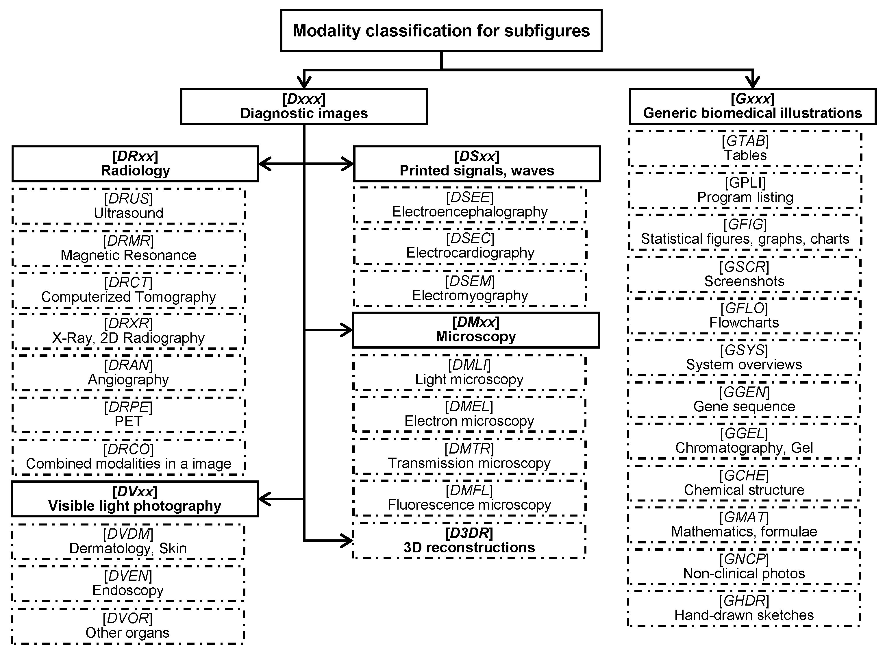
For our experiments, we utilize ImageCLEF2015 and ImageCLEF2016 subfigure classification datasets [33,34] created from a subset of PubMed Central. This task makes training data and test data available containing subfigures extracted from compound figures of the biomedical literatures in PubMed (see Figure 2). Similar to the modality classification task organized in ImageCLEF2013, thirty hierarchical modality classes proposed by [41], except for compound images (COMP), are used in subfigure classification task, shown in Figure 3. In ImageCLEF2015 [33], the training set contains 4532 figures and the test set 2244 figures. In ImageCLEF2016 [34], they expand the training set to 6776 figures and the test set to 4166 figures.
Before inputting figures into CNNs, we resize them to a square of 224 × 224 pixels. After loading an image into PIL (Python Imaging Library) format, we convert a PIL image instance to a NumPy array. Using preprocessing tools of Keras, we prepare inputs of shape for CNNs, where is the number of instances.
4.2. Baselines
This section describes the baseline methods, and their results in both ImageCLEF2015 and ImageCLEF2016.
FHDO BCSG [10,14]—The FHDO Biomedical Computer Science Group in the University of Applied Science and Arts, Dortmund—obtained the best visual result with an accuracy of 60.91% in ImageCLEF2015 labeled as Baseline_2015 (see Table 1). They extracted eight kinds of low-level features from image and fed them to a classifier of the multiclass linear kernel Support Vector Machine (SVM).
4.3. Expeimental Setup
We compare accuracies of three CNNs (CNN-6, VGGNet-16, ResNet-50) to baselines (Baseline_2015 and Baseline_2016) and also inspect the performance of our proposed model based on the voting system.
In accordance with the evaluation criterion of the benchmark, we evaluate our approach based on 30-classes of classification accuracy for all experiments, unless otherwise stated. Cross-validation is generally used to select the optimal CNN training parameters. Given that CNN training can take an extensive amount of time, we choose original small training set to implement fully independent experiments with 10-fold cross validation (10FCV) for model selection (see Table 1 and Table 2). But when training multiple CNNs on DS_Aug2, the number of epochs are reduced due to the fact that the running time is too long (see Section 4.4.3) and validation accuracy doesn’t change much after 5 epochs.
Most codes are modified from our previous work [22,35,36] and are implemented with the neural network library of Keras, running on top of Theano. After loading the Theano version of weights, not including the top layer(s), we add new full-connected layer(s) at the top of the CNNs (VGGNet-16 and ResNet-50) and initialize their weights using Glorot [37] uniform. All default parameters are used, except for those parameters mentioned in Section 2. Our networks are trained on one NVIDIA Tesla K20c GPU—4 G memories—in a 64 bit Dell computer with two 2.40 GHz CPUs, 64 G main memories, and Ubuntu 12.04.
4.4. Experimental Results and Discussion
4.4.1. Deep Transfer Learning
We obtained good performance [36] using CNN-6 in the Compound Figure Detection Task [33,34]. The first experiment of training CNN-6 from scratch (with random initialization) on the subfigure classification task is designed for rapidly getting results rather than optimal performance. Similar to our previous work [22,35,36], although combining more networks provides more performance gain, and considering the huge cost time of the training network on DS_Aug2 (described in Section 3.3), we train only 5 networks for each CNN. From Table 1 and Table 2, we can see that the results of CNN-6 are promising—66.13% in ImageCLEF2015 and 81.86% ImageCLEF2016. The results of CNN-6 demonstrate that it can capture domain-specific information from the medical dataset, which benefits from the training approach, even with only six weight layers.
Now that CNN-6 is effective in this task, we attempt to train deeper CNNs. We train five CNNs for each of CNN-6, VGGNet-16, or ResNet-50, using parameters described in Table 3.
Table 1 and Table 2 demonstrate that the performance of three CNNs exist in a positive correlation to the depth of the networks in all three datasets described in Section 3.3. These results give obvious evidence of the central importance of network depth. Both in ImageCLEF2015 and ImageCLEF2016, Resnet-50 has a higher accuracy than baseline, which indicates that it plays a leading role in our proposed model.
Unlike the similar accuracies in ImageCLEF2016, all pre-trained CNNs achieve better performance than the baseline method in ImageCLEF2015, although it uses several state-of-the-art traditional features engineering methods. Especially, CNN-6 with only six layers beat Baseline_2015, which provides more evidence that the feature learning method is also very effective in current task.
4.4.2. Data Augmentation
The original training set of the subfigure classification task in ImageCLEF2015 (4532 images) and in ImageCLEF2016 (6776 images) is much smaller than the ImageNet training set (about 1.2 million images). To address this problem, we augment the dataset from two perspectives: bringing new images into the original training set (DS_Aug1) and transforming original images (DS_Aug2).
By horizontal comparison of the results in Table 1 and Table 2, we find that our proposed model and three CNNs achieve higher accuracies after introducing new images (DS_Aug1) and create new label-preserved images (DS_Aug2). More evidence of the positive effects of the two data augmentation strategies is that ResNet-50 has surpassed the baseline, not only in ImageCLEF2015, but also in ImageCLEF2016 after expanding data. Specially, on the one hand, it is effective to increase the data variety to some extent by introducing figures from ImageCLEF2013 with single-modality, so accuracies of our proposed models increase by more than 3 percentage points (see Table 1 and Table 2). On the other hand, we implement image data transformation in real time with Keras API of the ImageDataGenerator, and use the following parameters: random rotations ([0, 20] degrees), random shift horizontally ([0, 20] of total width and height), random zoom ([80%, 120%]), and random flip horizontally and vertically. Although not performing transformation parameters tuning, our proposed model achieved acceptable results—accuracies increased from 76.07 to 76.87% in ImageCLEF2015, and from 86.07 to 87.37% in ImageCLEF2016 (see Table 1 and Table 2). There is room to improve the performance of our model when choosing parameters based on a grid search or introducing new transformation techniques.
Our proposed model takes advantage of the different depths of the networks and the two data augmentation methods to achieve better performances (76.78% in 2015 and 86.92% in 2016) than the baselines (60.91% in 2015 and 85.38% in 2016) described in Section 3.3. With weights of [0.1, 0.2, 0.7] based on the grid search, our fusion models achieve accuracies (76.87% and 87.37%) beyond baselines (60.91% and 85.38%) in ImageCLEF2015 and ImageCLEF2016.
4.4.3. Running Time
The running time of our networks is listed in Table 4. For comparative purposes, we present the running time on training or testing one sample from the DS_Original dataset, excluding data preprocessing, and record the training time in one epoch. Without surprise, we find that VGGNet-16 tends to need more running time than CNN-6 (see Table 4), because VGGNet-16 has more parameters. Although ResNet-50 has more layers, it relies on its advantage of having a smaller parameter size, and has a roughly equivalent training time to VGGNet-16, and a lower testing time.
At the same time, we record our training time of all the samples in one epoch on two expanded datasets. From Table 5, we can see that it takes much more time to train networks when applying common real-time data augmentation with rotation, zoom, shift, and flip transformation.
5. Conclusions
We have presented a model for medical image modality classification that is composed of three CNNs with different depths, which are combined by weighted averaging of the prediction probabilities. The depth of network is of central importance for current task, as is demonstrated by the dominance performance of ResNet in ImageCLEF2015 and ImageCLEF2016. Our proposed transfer learning method can benefit from generic features captured by CNNs pre-trained on ImageNet, and domain-specific features captured by the top layers of extremely deep CNNs and another “shallower” CNN, which are trained from scratch on medical images. Our model—based on this transfer learning method and two data augmentation strategies—could identify efficiently the modality of medical images. We hope to include more powerful CNNs such as ResNet with 152 layers or other new state-of-the-art models for image classification into our system, and to focus on improving the performance for this task. Furthermore, we plan to explore more complicated fusion strategies, such as using the MKL (Multiple Kernel Learning) algorithm to fuse models in feature level or introduce the synergic signal system to fuse results in the model level.
Acknowledgments
This research was supported by the National Natural Science Foundation of China (No. 61272373, No. 61202254, and No. 71303031), the Fundamental Research Funds for the Central Universities (No. DC13010313, No.DCPY2016077, Natural Science Foundation of Liaoning Province, China (201602195 and No. DC201502030202), and the Doctoral Scientific Research Foundation of Liaoning (NO. 201601084). The authors also gratefully acknowledge the helpful comments and suggestions of the reviewers, which improve the presentation.
Author Contributions
Yuhai Yu designed and wrote paper; Hongfei Lin supervised the work; Jiana Meng, Xiaocong Wei, and Hai Guo conceived and designed the experiments; Yuhai Yu and Zhehuan Zhao performed the experiments; Yuhai Yu analyzed the data. All authors have read and approved the final manuscript.
Conflicts of Interest
The authors declare no conflict of interest.
References
- Lu, Z. PubMed and beyond: A survey of web tools for searching biomedical literature. Database 2011. [Google Scholar] [CrossRef] [PubMed]
- Khan, F.F.; Saeed, A.; Haider, S.; Ahmed, K.; Ahmed, A. Application of medical images for diagnosis of diseases-review article. World J. Microbiol. Biotechnol. 2017, 2, 135–138. [Google Scholar]
- Shi, J.; Zheng, X.; Li, Y.; Zhang, Q.; Ying, S. Multimodal Neuroimaging Feature Learning with Multimodal Stacked Deep Polynomial Networks for Diagnosis of Alzheimer’s Disease. IEEE J. Biomed. Health Inform. 2017. [Google Scholar] [CrossRef] [PubMed]
- Shi, J.; Wu, J.; Li, Y.; Zhang, Q.; Ying, S. Histopathological image classification with color pattern random binary hashing based PCANet and matrix-form classifier. IEEE J. Biomed. Health Inform. 2016. [Google Scholar] [CrossRef] [PubMed]
- De Herrera, A.G.S.; Kalpathy-Cramer, J.; Fushman, D.D.; Antani, S.; Müller, H. Overview of the ImageCLEF 2013 medical tasks. In Proceedings of the Working Notes of CLEF, Valencia, Spain, 23–26 September 2013. [Google Scholar]
- Müller, H.; Michoux, N.; Bandon, D.; Geissbuhler, A. A review of content-based image retrieval systems in medical applications—Clinical benefits and future directions. Int. J. Med. Inform. 2004, 73, 1–23. [Google Scholar] [CrossRef] [PubMed]
- Demner-Fushman, D.; Antani, S.; Simpson, M.; Thoma, G.R. Design and development of a multimodal biomedical information retrieval system. J. Comput. Sci. Eng. 2012, 6, 168–177. [Google Scholar] [CrossRef]
- Tirilly, P.; Lu, K.; Mu, X.; Zhao, T.; Cao, Y. On modality classification and its use in text-based image retrieval in medical databases. In Proceedings of the 9th International Workshop on Content-Based Multimedia Indexing (CBMI) 2011, Madrid, Spain, 13–15 June 2011. [Google Scholar]
- De Herrera, A.G.S.; Markonis, D.; Müller, H. Bag-of-Colors for Biomedical Document Image Classification. In Medical Content-Based Retrieval for Clinical Decision Support (MCBR-CDS) 2012, Lecture Notes in Computer Science; Springer: Berlin/Heidelberg, Germany, 2013. [Google Scholar]
- Pelka, O.; Friedrich, C.M. FHDO biomedical computer science group at medical classification task of ImageCLEF 2015. In Proceedings of the Working Notes of CLEF, Toulouse, France, 8–11 September 2015. [Google Scholar]
- Cirujeda, P.; Binefa, X. Medical Image Classification via 2D color feature based Covariance Descriptors. In Proceedings of the Working Notes of CLEF, Toulouse, France, 8–11 September 2015. [Google Scholar]
- Valavanis, L.; Stathopoulos, S.; Kalamboukis, T. IPL at CLEF 2016 Medical Task. In Proceedings of the Working Notes of CLEF, Évora, Portugal, 5–8 September 2016. [Google Scholar]
- Li, P.; Sorensen, S.; Kolagunda, A.; Jiang, X.; Wang, X.; Kambhamettu, C.; Shatkay, H. UDEL CIS Working Notes in ImageCLEF 2016. In Proceedings of the Working Notes of CLEF, Évora, Portugal, 5–8 September 2016. [Google Scholar]
- Pelka, O.; Friedrich, C.M. Modality prediction of biomedical literature images using multimodal feature representation. GMS Med. Inform. Biom. Epidemiol. 2016, 12. [Google Scholar] [CrossRef]
- Bengio, Y.; Courville, A.; Vincent, P. Representation learning: A review and new perspectives. IEEE Trans. Pattern Anal. Mach. Intell. 2013, 35, 1798–1828. [Google Scholar] [CrossRef] [PubMed]
- Krizhevsky, A.; Sutskever, I.; Hinton, G.E. Imagenet classification with deep convolutional neural networks. In Proceedings of the Advances in Neural Information Processing Systems, Lake Tahoe, NV, USA, 3–6 December 2012. [Google Scholar]
- Simonyan, K.; Zisserman, A. Very deep convolutional networks for large-scale image recognition. Comput. Sci. 2014; arXiv:1409.1556. [Google Scholar]
- Szegedy, C.; Liu, W.; Jia, Y.; Sermanet, P.; Reed, S.; Anguelov, D.; Erhan, D.; Vanhoucke, V.; Rabinovich, A. Going deeper with convolutions. In Proceedings of the IEEE Conference on Computer Vision and Pattern Recognition, Hynes Convention Center, Boston, MA, USA, 7–12 June 2015. [Google Scholar]
- He, K.; Zhang, X.; Ren, S.; Sun, J. Deep residual learning for image recognition. In Proceedings of the IEEE Conference on Computer Vision and Pattern Recognition, Seattle, WA, USA, 27–30 June 2016. [Google Scholar]
- Russakovsky, O.; Deng, J.; Su, H.; Krause, J.; Satheesh, S.; Ma, S.; Huang, Z.; Karpathy, A.; Khosla, A.; Bernstein, M.; Berg, A.C.; Li, F.F. Imagenet large scale visual recognition challenge. Int. J. Comput. Vis. 2015, 115, 211–252. [Google Scholar] [CrossRef]
- LeCun, Y.; Bengio, Y.; Hinton, G. Deep learning. Nature 2015, 521, 436–444. [Google Scholar] [CrossRef] [PubMed]
- Yu, Y.; Lin, H.; Meng, J.; Zhao, Z.; Li, Y.; Zuo, L. Modality classification for medical images using multiple deep convolutional neural networks. J. Colloid Interface Sci. 2015, 11, 5403–5413. [Google Scholar] [CrossRef]
- Ravishankar, H.; Sudhakar, P.; Venkataramani, R.; Thiruvenkadam, S.; Annangi, P.; Babu, N.; Vaidya, V. Understanding the Mechanisms of Deep Transfer Learning for Medical Images. In Deep Learning and Data Labeling for Medical Applications. Lecture Notes in Computer Science; Springer International Publishing: Cham, Switzerland, 2016; pp. 188–196. [Google Scholar]
- Shin, H.C.; Roth, H.R.; Gao, M.; Lu, L.; Xu, Z.; Nogues, I.; Yao, J.; Mollura, D.; Summers, R.M. Deep convolutional neural networks for computer-aided detection: CNN architectures, dataset characteristics and transfer learning. IEEE Trans. Med. Imaging 2016, 35, 1285–1298. [Google Scholar] [CrossRef] [PubMed]
- Kumar, A.; Kim, J.; Lyndon, D.; Fulham, M.; Feng, D. An ensemble of fine-tuned convolutional neural networks for medical image classification. IEEE J. Biomed. Health Inform. 2017, 21, 31–40. [Google Scholar] [CrossRef] [PubMed]
- Zhang, J.; Xia, Y.; Wu, Q.; Xie, Y. Classification of Medical Images and Illustrations in the Biomedical Literature Using Synergic Deep Learning. Comput. Sci. 2017; arXiv:1706.09092. [Google Scholar]
- Koitka, S.; Friedrich, C.M. Traditional feature engineering and deep learning approaches at medical classification task of ImageCLEF 2016. In Proceedings of the Working Notes of CLEF, Évora, Portugal, 5–8 September 2016. [Google Scholar]
- Donahue, J.; Jia, Y.; Vinyals, O.; Hoffman, J.; Zhang, N.; Tzeng, E.; Darrell, T. Decaf: A deep convolutional activation feature for generic visual recognition. In Proceedings of the International Conference on Machine Learning, Beijing, China, 21–26 June 2014. [Google Scholar]
- Lowe, D.G. Distinctive image features from scale-invariant keypoints. Int. J. Comput. Vis. 2004, 60, 91–110. [Google Scholar] [CrossRef]
- Wengert, C.; Douze, M.; Jégou, H. Bag-of-colors for improved image search. In Proceedings of the 19th ACM International Conference on Multimedia, New York, NY, USA, 28 November–1 December 2011. [Google Scholar] [CrossRef] [Green Version]
- Yang, J.; Jiang, Y.G.; Hauptmann, A.G.; Ngo, C.W. Evaluating bag-of-visual-words representations in scene classification. In Proceedings of the International Workshop on ACM Multimedia Information Retrieval, University of Augsburg, Augsburg, Germany, 28–29 September 2007. [Google Scholar]
- Yin, X.; Düntsch, I.; Gediga, G. Quadtree representation and compression of spatial data. Trans. Rough Sets XIII 2011, 207–239. [Google Scholar] [CrossRef]
- De Herrera, A.G.S.; Müller, H.; Bromuri, S. Overview of the ImageCLEF 2015 medical classification task. In Proceedings of the Working Notes of CLEF, Toulouse, France, 8–11 September 2015. [Google Scholar]
- De Herrera, A.G.S.; Schaer, R.; Bromuri, S.; Müller, H. Overview of the ImageCLEF 2016 medical task. In Proceedings of the Working Notes of CLEF, Évora, Portugal, 5–8 September 2016. [Google Scholar]
- Yu, Y.; Lin, H.; Meng, J.; Zhao, Z. Visual and Textual Sentiment Analysis of a Microblog Using Deep Convolutional Neural Networks. Algorithms 2016, 9, 41. [Google Scholar] [CrossRef]
- Yu, Y.; Lin, H.; Meng, J.; Wei, X.; Zhao, Z. Assembling Deep Neural Networks for Medical Compound Figure Detection. Information 2017, 8, 48. [Google Scholar] [CrossRef]
- Glorot, X.; Bengio, Y. Understanding the difficulty of training deep feedforward neural networks. In Proceedings of the 13th International Conference on Artificial Intelligence and Statistics (AISTATS), Sardinia, Italy, 13–15 May 2010. [Google Scholar]
- Kingma, D.; Ba, J. Adam: A method for stochastic optimization. Comput. Sci. 2014; arXiv:1412.6980. [Google Scholar]
- Kuncheva, L.I.; Rodríguez, J.J. A weighted voting framework for classifiers ensembles. Knowl. Inf. Syst. 2014, 38, 259. [Google Scholar] [CrossRef]
- Chen, D.; Riddle, D.L. Function of the PHA-4/FOXA transcription factor during C. elegans post-embryonic development. BMC Dev. Biol. 2008, 8, 26. [Google Scholar] [CrossRef] [PubMed]
- Müller, H.; Kalpathy-Cramer, J.; Demner-Fushman, D.; Antani, S. Creating a classification of image types in the medical literature for visual categorization. In Proceedings of the SPIE Medical Imaging, San Francisco, CA, USA, 21–26 January 2012. [Google Scholar]
Figure 1.
Architecture of our proposed model for subfigure classification. Deep CNNs are denoted as “network name-(depth)”.
Figure 1.
Architecture of our proposed model for subfigure classification. Deep CNNs are denoted as “network name-(depth)”.
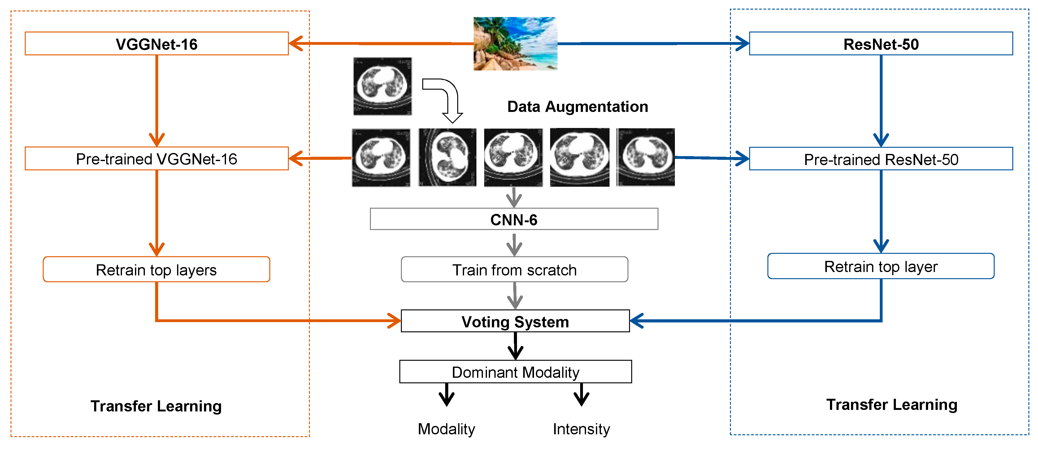
Figure 2.
Example of medical figures with different modalities in a biomedical article [40]. ImageCLEF provides subfigures extracted from these compound figures in the subfigure classification task. (A) pha-4 RNAi treatment efficiently inhibits pha-4 transcription. Semi-quantitative RT-PCR shows pha-4 and rpl-21 transcription levels in daf-7(e1372) and daf-2(e1370) dauer larvae treated with the RNAi control (lanes 1, 3) and pha-4 RNAi (lanes 2, 4). RT-PCR experiments were performed three times with consistent results using three independent RNA preparations. (B) PHA-4 is needed for dauer recovery. Dauer larvae formed constitutively at 25 °C in the presence of pha-4 RNAi from hatching showed significantly decreased recovery upon downshift to 15 °C compared to control daf-7(e1372), daf-1(m40), daf-2(e1370), and age-1(m865) mutants. Percentages of dauer recovery, numbers of animals scored, and p values for t-tests were shown in Table 1 [40]. The entire experiment was performed twice with triplicates for each treatment. (C-F) pha-4 is involved in gonad and vulva development. (C) Control post-dauer daf-7(e1372) adult; (D) pha-4 RNAi-treated post-dauer daf-7(e1372) adult; (E) control post-dauer daf-2(e1370) adult; (F) pha-4 RNAi-treated post-dauer daf-2(e1370) adult.
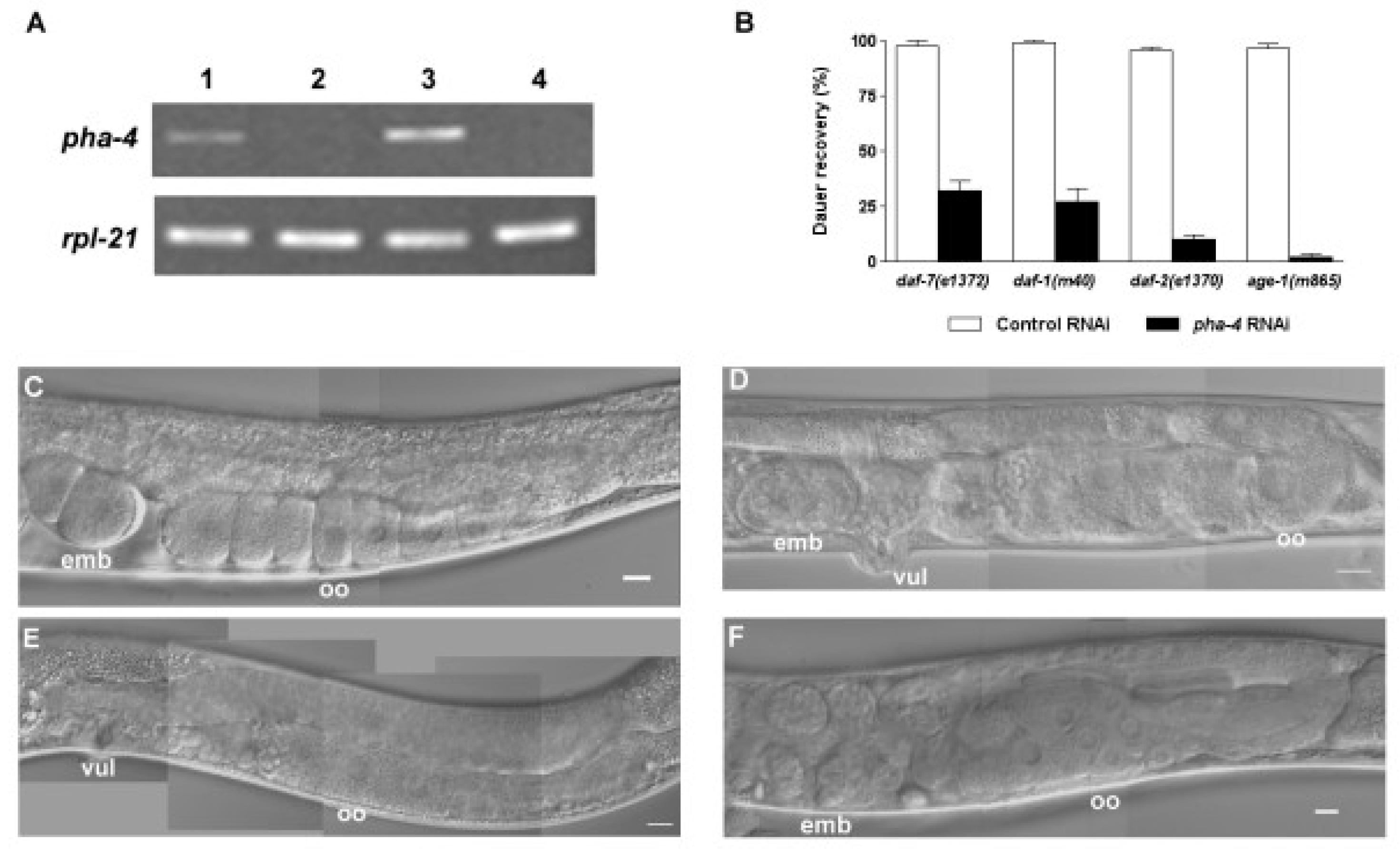
Figure 3.
Thirty modality classes, along with the class codes in brackets.

Table 1.
Accuracy of visual methods in ImageCLEF2015.
| Methods | 10FCV | Evaluation | ||
|---|---|---|---|---|
| DS_Original | DS_Original | DS_Aug1 | DS_Aug2 | |
| Baseline_2015 [10,14] | - | - | 60.91 | - |
| CNN-6 | 59.95 | 57.09 | 58.33 | 66.13 |
| VGGNet-16 | 87.27 | 67.83 | 70.50 | 71.61 |
| ResNet-50 | 89.34 | 72.10 | 75.75 | 76.78 |
| Our proposed model | 90.22 | 72.42 | 76.07 | 76.87 |
Table 2.
Accuracy of visual methods in ImageCLEF2016.
| Methods | 10FCV | Evaluation | ||
|---|---|---|---|---|
| DS_Original | DS_Original | DS_Aug1 | DS_Aug2 | |
| Baseline_2016 [23] | - | - | 85.38 | - |
| CNN-6 | 75.87 | 70.67 | 74.70 | 81.86 |
| VGGNet-16 | 85.13 | 78.99 | 81.73 | 83.54 |
| ResNet-50 | 87.47 | 82.51 | 85.25 | 86.92 |
| Our proposed model | 88.40 | 82.61 | 86.07 | 87.37 |
Table 3.
Training parameters in ImageCLEF2015 and ImageCLEF2016.
| CNNs | Epochs | Learning Rate | Batch Size | |||
|---|---|---|---|---|---|---|
| 10FCV | DS_Original | DS_Aug1 | DS_Aug2 | |||
| CNN-6 | 25 | 25 | 25 | 5 | 0.001 | 32 |
| VGGNet-16 | 15 | 15 | 15 | 5 | 0.0002 | 32 |
| ResNet-50 | 30 | 30 | 30 | 5 | 0.0002 | 32 |
Table 4.
Training and testing time of CNNs on DS_Original dataset.
| Methods | Training (ms) | Test (ms) |
|---|---|---|
| CNN-6 | 18.2 | 4 |
| VGGNet-16 | 28.4 | 20.5 |
| ResNet-50 | 29 | 10.7 |
Table 5.
Training time of CNNs on augmented dataset.
| Methods | ImageCLEF2015 (s) | ImageCLEF2016 (s) | ||
|---|---|---|---|---|
| DS_Aug1 | DS_Aug2 | DS_Aug1 | DS_Aug2 | |
| CNN-6 | 143 | 4315 | 170 | 4688 |
| VGGNet-16 | 224 | 5757 | 280 | 6299 |
| ResNet-50 | 229 | 6532 | 267 | 7112 |
© 2017 by the authors. Licensee MDPI, Basel, Switzerland. This article is an open access article distributed under the terms and conditions of the Creative Commons Attribution (CC BY) license (http://creativecommons.org/licenses/by/4.0/).
Share and Cite
MDPI and ACS Style
Yu, Y.; Lin, H.; Meng, J.; Wei, X.; Guo, H.; Zhao, Z. Deep Transfer Learning for Modality Classification of Medical Images. Information 2017, 8, 91. https://doi.org/10.3390/info8030091
AMA Style
Yu Y, Lin H, Meng J, Wei X, Guo H, Zhao Z. Deep Transfer Learning for Modality Classification of Medical Images. Information. 2017; 8(3):91. https://doi.org/10.3390/info8030091
Chicago/Turabian StyleYu, Yuhai, Hongfei Lin, Jiana Meng, Xiaocong Wei, Hai Guo, and Zhehuan Zhao. 2017. "Deep Transfer Learning for Modality Classification of Medical Images" Information 8, no. 3: 91. https://doi.org/10.3390/info8030091
Note that from the first issue of 2016, this journal uses article numbers instead of page numbers. See further details here.