A Practical Point Cloud Based Road Curb Detection Method for Autonomous Vehicle


1
School of Engineering, Anhui Agriculture University, Hefei 230036, China
2
School of Automotive and Transportation Engineering, Hefei University of Technology, Hefei 230009, China
3
Department of Automation, University of Science and Technology of China, Hefei 230026, China
4
Institute of Applied Technology, Hefei Institutes of Physical Science, Chinese Academy of Sciences, Hefei 230031, China
5
Ma’anshan Power Supply Company, Ma’anshan 243000, China
*
Author to whom correspondence should be addressed.
Information 2017, 8(3), 93; https://doi.org/10.3390/info8030093
Submission received: 22 May 2017
/
Revised: 21 July 2017
/
Accepted: 21 July 2017
/
Published: 30 July 2017
(This article belongs to the Special Issue Intelligent Transportation Systems)
Abstract
:Robust and quick road curb detection under various situations is critical in developing intelligent vehicles. However, the road curb detection is easily affected by the obstacles in the road area when Lidar based method is applied. A practical road curb detection method using point cloud from a three-dimensional Lidar for autonomous vehicle is reported in this paper. First, a multi-feature, loose-threshold, varied-scope ground segmentation method is presented to increase the robustness of ground segmentation with which obstacles above the ground can be detected. Second, the road curb is detected by applying the global road trend and an extraction-update mechanism. Experiments show the robustness and efficiency of the road curb detection under various environments. The road curb detection method is 10 times the speed of traditional method and the accuracy is much higher than existing methods.
1. Introduction
Environment perception is an indispensable component for autonomous vehicle as it provides real-time environment information. Driving safety and intelligence of autonomous vehicle is based on accurate and quick understanding of the driving environment. Among the elements that consist the driving environment, road curbs are especially important for being boundaries of the drivable area.
To detect road curbs quickly and accurately, a variety of sensors are used including cameras and lasers. In the past decades, great achievements have been made in computer vision and some of the proposed methods have been successfully applied to detect lane marks, traffic participants and traffic signs including vehicle, bicycle and pedestrian, and traffic lights [1,2,3,4,5,6,7,8]. However cameras are sensitive to light changes and no distance information is provided. Compared with cameras, Lidars can provide accurate distance information and they are not affected by light conditions. 2D-Lidars were widely used to detect obstacles in advanced driver assistant system on vehicles [9]. While the data is too sparse for environment perception of autonomous vehicles. In recent researches on autonomous vehicles, 3D Lidar plays a more and more import role as it provides sufficient information, in the form of point cloud, to model the 3D environment. 3D Lidar is a kind of multi-beam Lidar which percept the environment by transmitting and receiving multiple laser rays. In 2005 DARPA Grand Challenge, only the team from Velodyne, a famous 3D Lidar manufacturer, was equipped with a 3D Lidar. While 6 of the 11 teams entered the final competition of 2007 DARPA Urban Challenge were equipped with a 3D Lidar [10,11]. Recently, Google, Ford and Baidu choose 3D Lidars as the main sensor to obtain environment information [12,13,14,15,16].
Ground segmentation is another way of saying obstacle detection. Height difference based methods were proposed to detect obstacles [17,18,19,20,21]. Besides, a combination of height difference and convexity criterion was proposed to segment the ground in [22]. Cheng et al. [23] proposed a Ring Gradient-based Local Optimal Segmentation (RGLOS) algorithm to segment the ground based on the gradient feature between the rings. The common problem for the aforementioned method is that a single or multiple features are adopted in ground segmentation, resulting in over segmentation with strict threshold while under-segmentation with loose threshold. To overcome this shortcoming, ground segmentation method based on the multi-feature with loose threshold is presented in [24]. These two methods take advantage of local road features to detect curbs without considering the global road trend. However, our experiment found that the applied scope of different features should be considered in greater detail because the geometric properties vary with different features.
Road curbs can be deemed as special obstacles which are boundaries of the drivable area. Chen et al. [25] selected the initial curb points from the individual scan lines by using the distance criterion, Hough Transform (HT), and the iterative Gaussian Process Regression (GPR). Zhao [26] obtained the seed points that meet three criteria and modeled the curb as a parabola while using a random sample consensus (RANSAC) algorithm to remove the false positives that do not match the parabolic model. Least trimmed squares (LTS) regression method is applied to fit a function in the curb candidate points in [27] while a sliding window is applied to obtain curb points in [28]. In the study of Liu et al. [24], distance transformation is performed on the obstacle map and threshold segmentation is used to increase the continuity of the map. Thereafter, the drivable area is obtained by region growing, and the road curb points are obtained by searching. All the aforementioned methods shared the drawback of being easily affected by the obstacle inside the road area, especially for road with considerable number of vehicles, because of the lack of the overall road shape information. They are based on local features of the road rather than the global road trend.
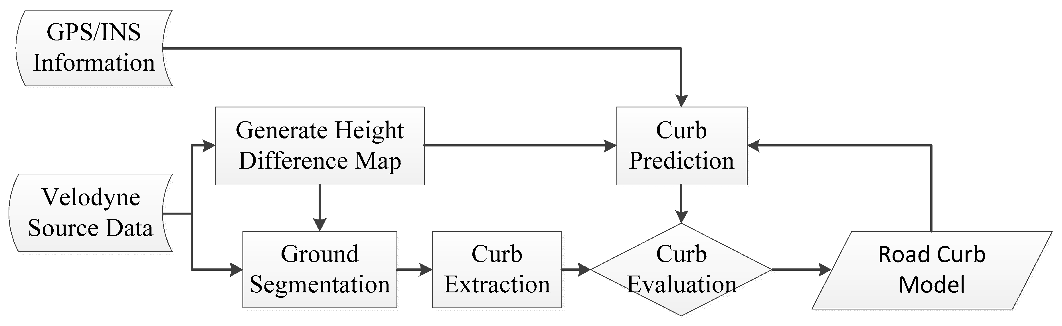
Based on the aforementioned considerations, a road curb detection method, which takes global trend of road curb into consideration, is proposed in this study and shown in Figure 1. First, a multi-feature, loose-threshold, varied-scope ground segmentation method is presented in this work. Features used in the segmentation process are discussed in detail. Second, a road curb detection process is proposed. The road curb can be obtained through extraction or tracking, which is switched by evaluating the predicted road curb. If the predicted road curb based on the motion of the vehicle is evaluated to be the right curb, then a simple update of the road curb is sufficient. Otherwise, the road curb should be obtained through extraction.
The main contributions of this work are threefold. First, a multi-feature, loose-threshold, varied-scope ground segmentation method is presented to increase the robustness of ground segmentation. Second, a road curb extraction method based on the analysis of the road shape information, which consists of road trend information and road width distribution information, is proposed. Third, a framework for road curb detection is proposed based on the multi-index evaluation of the road curb in three aspects, namely, the shape of the road curb, the fit degree between the road curb and the scene, and the variance between the curve and history information.
The succeeding portions of this paper are organized as follows: The segmentation of the ground is described in Section 2. The road curb detection method is discussed in Section 3. Experiment and results are introduced in Section 4. Section 5 provides our conclusions on this method and discusses future work that needs to be completed.
2. Ground Segmentation
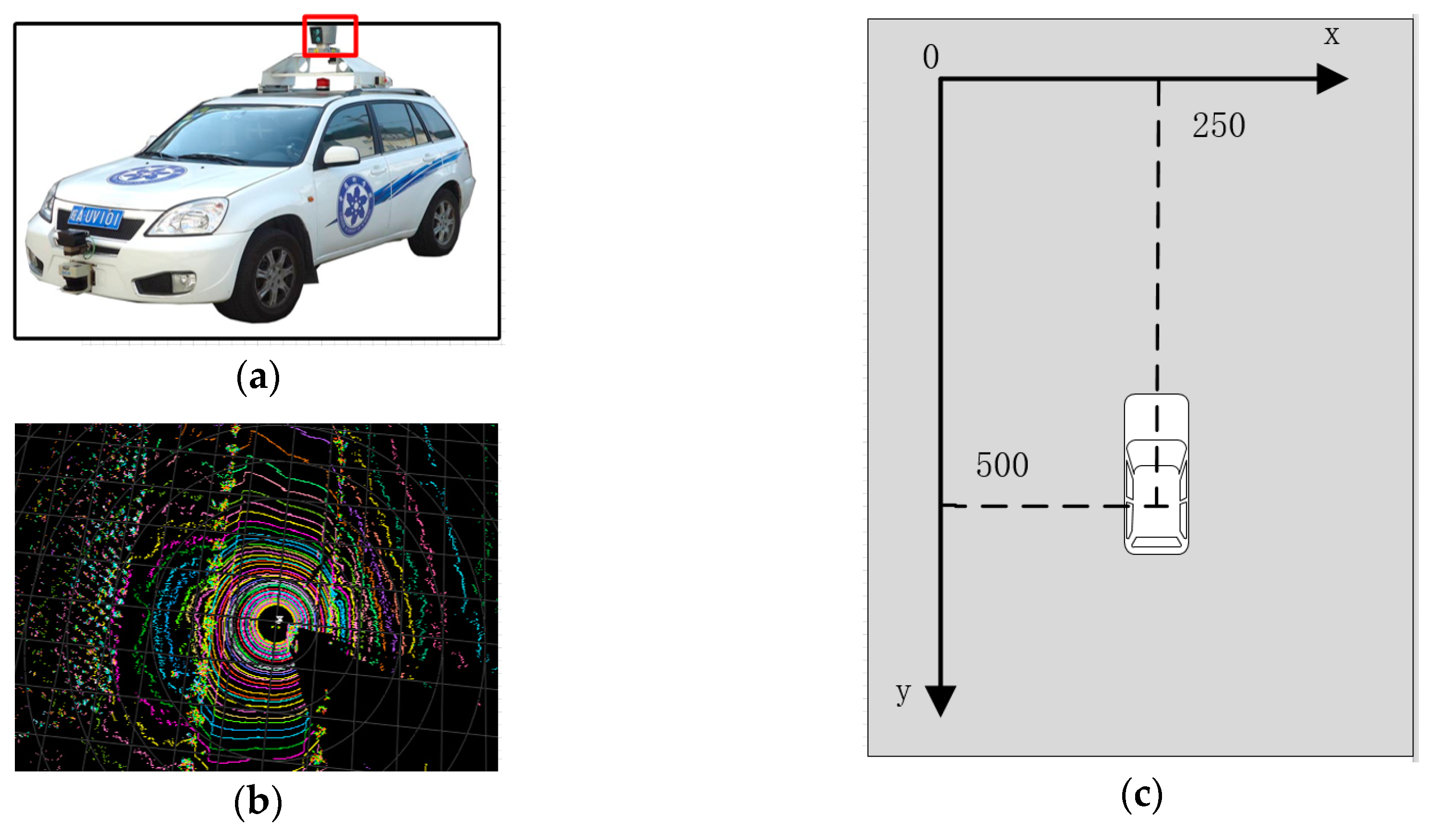
The experimental platform and a point cloud are shown in Figure 2. A Velodyne 3D-Lidar, which contains 64 laser transmitters, is mounted on the top of the vehicle. Each laser transmitter returns 1800 points per frame and they form a circle after projecting the points onto the horizontal plane. As a build-in feature of the Velodyne 3D-Lidar, the projected circles will be broken if obstacles are detected. Thus, ground segmentation can be completed by removing the continuous part of the circles. While the road surfaces are not entirely flat and the effects of different laser transmitters are different as a result of different scan ranges. It is difficult to segment the ground with a single feature because of the difficulty in definition of feature threshold. Strict or loose threshold will result in a low accuracy. Moreover, the scope should be considered as different features have different geometric properties. Based on the aforementioned considerations, a philosophy for multi-feature based ground segmentation is proposed. Features are analyzed and tested in various driving environments. Then the distinctive and robust ones will be applied in ground segmentation. Threshold and scope are set to remove as many ground points as possible while ensuring that no obstacle point is removed. The geometric characteristic of the remaining ground points is analyzed, and new features are constructed to remove the remaining ground points. After extensive experiments under various environments, features adopted in this study are discussed in the subsequent subsections.
2.1. Maximum Height Difference in One Grid (MaxHD)
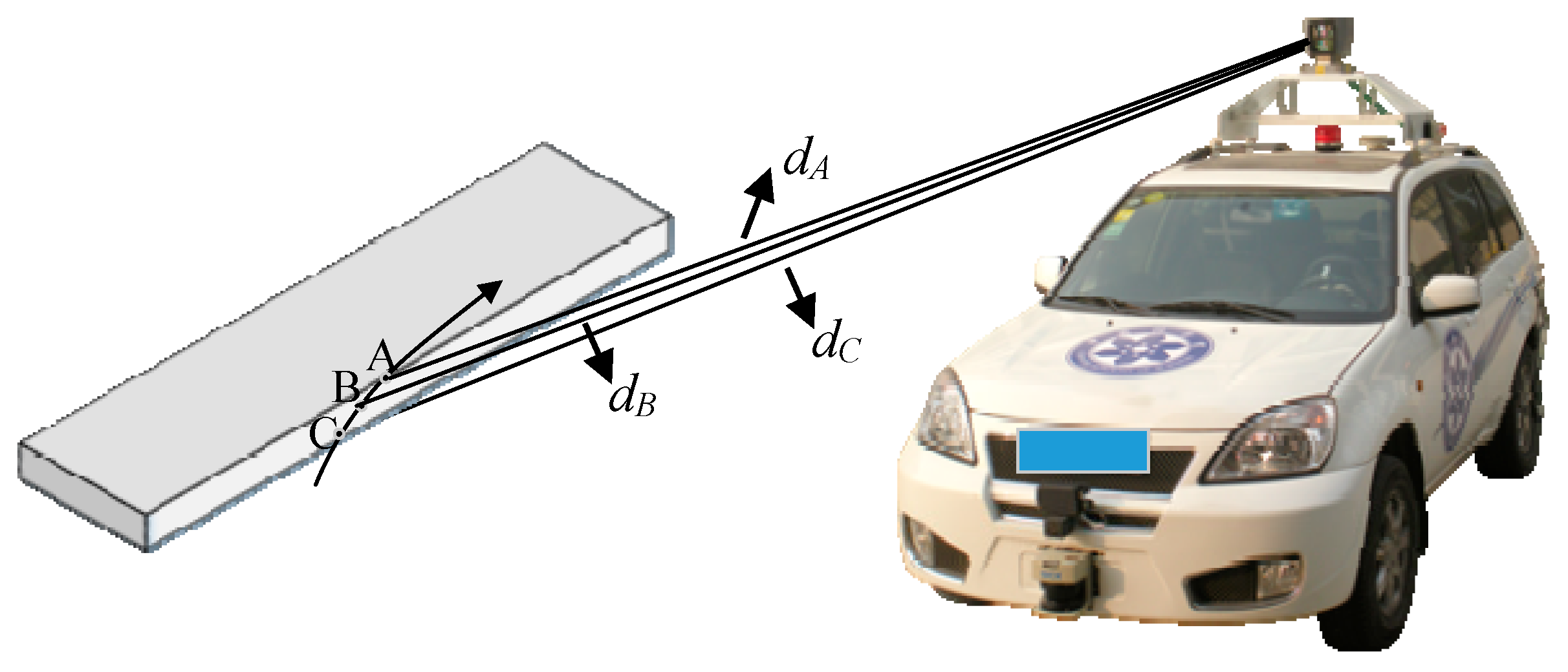
A 750 × 500 grid map can be obtained by projecting the point cloud onto the horizontal plane and the resolution is 20 cm × 20 cm. The local coordinate is shown in Figure 2c and the origin of the map is set as the left top point of the map. The Lidar is placed in (500, 250), thus, a range of 150 m × 100 m is covered. The maximum height difference is calculated by comparing the highest point and the lowest point projected onto the same grid cell, which is small in a flat area. However, our experiments show that this feature is not effective for wet ground and distant low obstacles. The height measurement of the point from wet ground is inaccurate and many laser points are lost as mirror reflection. When points are projected onto the distant low obstacle, the height change in one grid cell is excessively small, as illustrated in Figure 3.
In Figure 3, A–C are points on a distant low curb. The height difference of the three points is too small to be used to detect obstacles. Figure 4 shows an example of the failure of the feature of maximum height difference in a grid cell. Figure 4a shows that the experimental scene is a wide road with low stone curbs, which are approximately 10 cm high. Figure 4b shows the grid map generated from a frame of Velodyne raw data whose partially enlarged detail map is shown in Figure 4c. The figure shows that a segment of the distant stone curb is scanned by only one beam consisting of 10 pixels with an accumulated height difference of approximately 10 cm. The average height difference of one pixel is approximately 1 cm. Thus, it is difficult to distinguish the points and ground points with maximum height difference feature.
2.2. Tangential Angle Feature (TangenAngle)
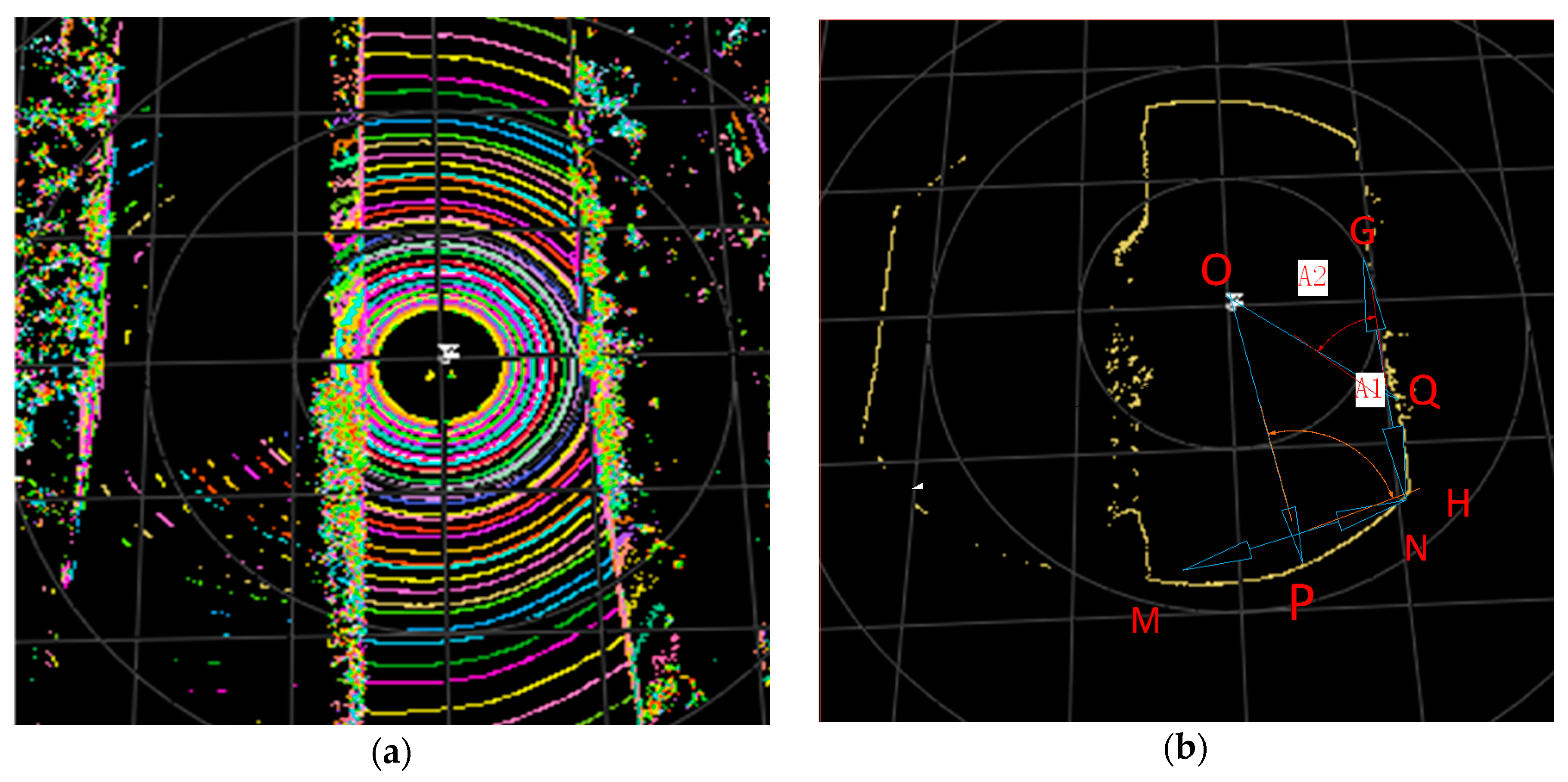
This feature is described in [23] which can be obtained with radial and tangential angle as shown in Figure 5. The Lidar is positioned on O and P is a point on road. Q is an obstacle point. The radial direction of P is represented with and tangential direction is represented with . M and N are adjacent points of P on both sides. Thus, the tangential angles for P and Q in Figure 5 are A1 and A2, respectively, and the cosine value of the tangential angle is calculated with (1) for P.
Figure 5 shows that, when a point is projected onto the ground, e.g., P, the value of AngleFeature is approximately 0 because the two directions are nearly vertical. By contrast, when a point is projected onto the obstacle, e.g., Q, the value of AngleFeature is higher because the angle between the two directions is acute.
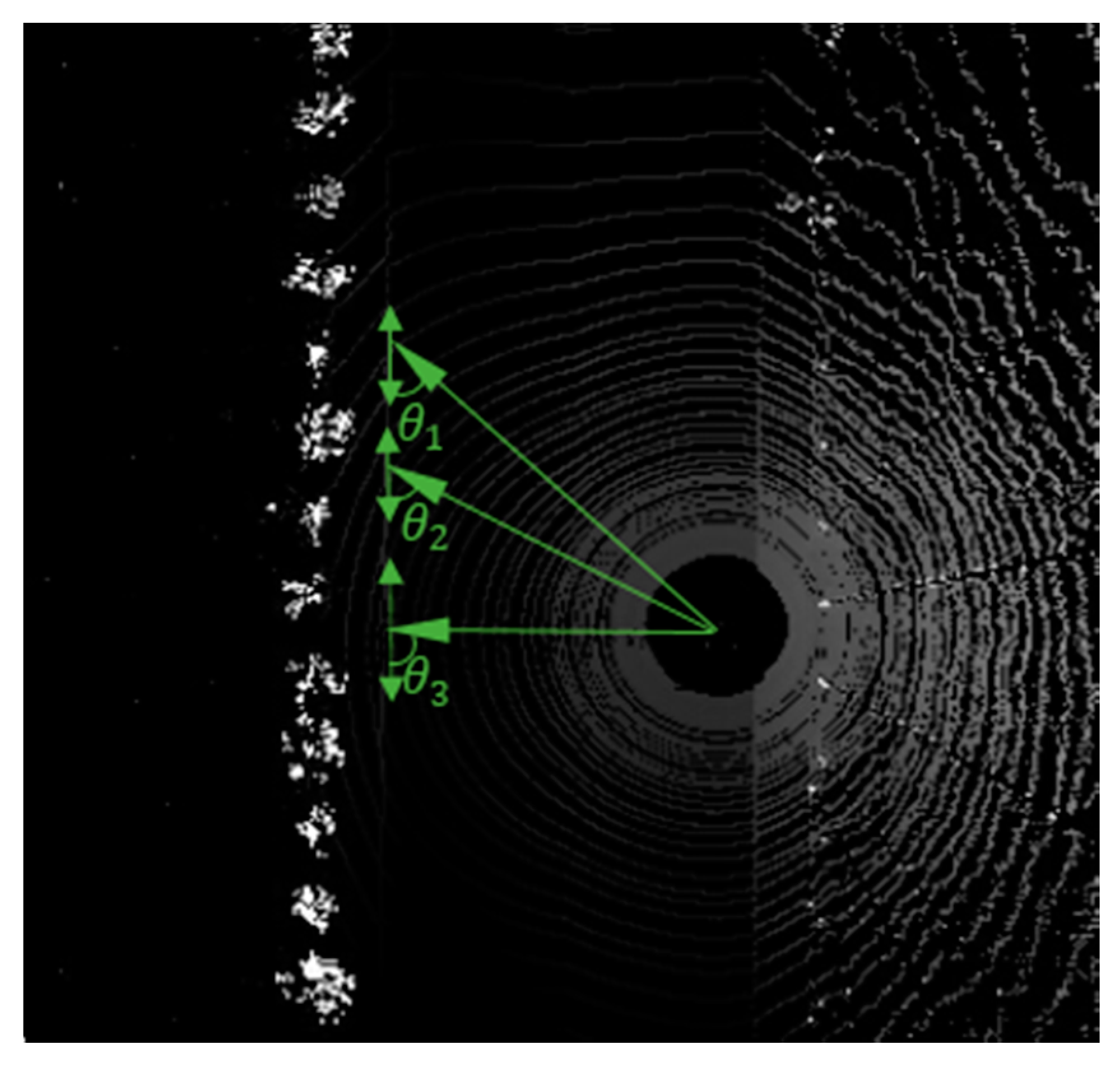
However, our experiment found that this feature is unsuitable for the points in the two sides of the vehicle because the value of AngleFeature is approximately 0 even if the points are projected onto the obstacle. The schematic diagram is shown in Figure 6.
Figure 6 shows three points on the road curb whose tangential angles are , and . Point 3 is found on the side direction of the vehicle, so AngleFeature is approximately 0 even if it is projected on the obstacle. The tangential angle becomes smaller when the points become farther away from the LIDAR, e.g., . Thus, the value of AngleFeature becomes larger, which means that this feature is more significant for far away points.
2.3. Change in Distance between Neighboring Points in One Spin (RadiusRatio)
When projected onto the flat ground, the points generated by one beam form a circle which means that the distance of the neighboring points are nearly the same. However, the distance becomes smaller when point is projected onto the positive obstacle (e.g., a bump) while lager when points are projected onto the negative obstacle (e.g., a pothole).
2.4. Height Difference Based on the Prediction of the Radial Gradient (HDInRadius)
Points A–C are three points obtained by three adjacent beams in one direction. The following equation will be satisfied if A, B and C are on the same plane.
where , , and are the heights of A, B, and C, respectively; is the distance of projection of B and C on the horizontal plane and is the distance of projection of A and B on the horizontal plane. Thus, can be predicted with and .
In Figure 7, C is projected onto the obstacle while A and B are projected onto the ground. is the height difference based on the prediction of the radial gradient of C and can be calculated as follows:
where should be 0 if C is projected onto the ground instead of the obstacle.
2.5. Selection of the Threshold and Scope for Each Feature
An experiment is performed by analyzing the value of each feature in a crossroad, where the road area is relatively broader than the normal straight road. The result is shown in Figure 8, where values of the four features are illustrated in a–d, respectively.
Figure 8a shows that the feature of maximum height difference in one grid cell near the vehicle is more distinguishable because the number of the points projected onto one grid is larger. Thus, the height variation in one grid cell can be reflected. On the contrary, the feature becomes less distinguishable, which means that the feature should be applied to the points near the vehicle.
As the road is not entirely flat, a sudden change in the direction of the points generated by one beam in a circle occurred, causing the sudden change of the tangential angle in the middle of the road, as shown in Figure 8b. Moreover, as shown in the red box, some laser beams shoot on the body of the autonomous vehicle and feature values of their tangential neighboring points in one spin change significantly which can be seen in Figure 8c too. Thus, the criterion of obstacles is satisfied and misdetection occurs.
The points generated by one beam in one spin are shown in Figure 8, where a section of points is blocked by an obstacle. Point O is the position of the LIDAR. Point Q is an obstacle point while points M and P are ground points. P and Q and adjacent points of M on both sides. The tangential angle of point M formed by and is an acute angle now instead of the normal right angle for the points projected onto the ground.
The distance change feature in one spin can also be influenced by the block of the obstacle, as shown in Figure 8 and Figure 9. As shown in Figure 8, the feature can be calculated as OP/OQ for point M, which should have been approximated to 1 for the points projected onto the ground because of the continuity of the points in one spin. However the value varied because of the block of the obstacle. Moreover, as mentioned previously, this feature also suffers the drawback of misdetection of the low obstacle. As shown in Figure 7d, the height difference based on the prediction of the radial gradient performs distinguishing in all scopes. However, because of the bump of the vehicle, noise may exist in the ground area.
The threshold and the applied scope for each feature are shown in Table 1. The definition of thresholds is difficult as the absence of ground truth of ground segmentation. We adopted an experimental method to find appropriate thresholds. The thresholds are adjusted and tested to obtain better performance in typical scenes including urban scene, field scenes which are introduced in the experimental part. After defining the thresholds, the four features are used in a cascade fashion. Points will be classified as obstacles if they satisfy all the four features. Otherwise, they will be treated as ground points.
3. Road Curb Detection
The height of curbs and distance between curbs and the sensor make it difficult to detect the curbs. However, the application of road trend can be helpful in the detection process.
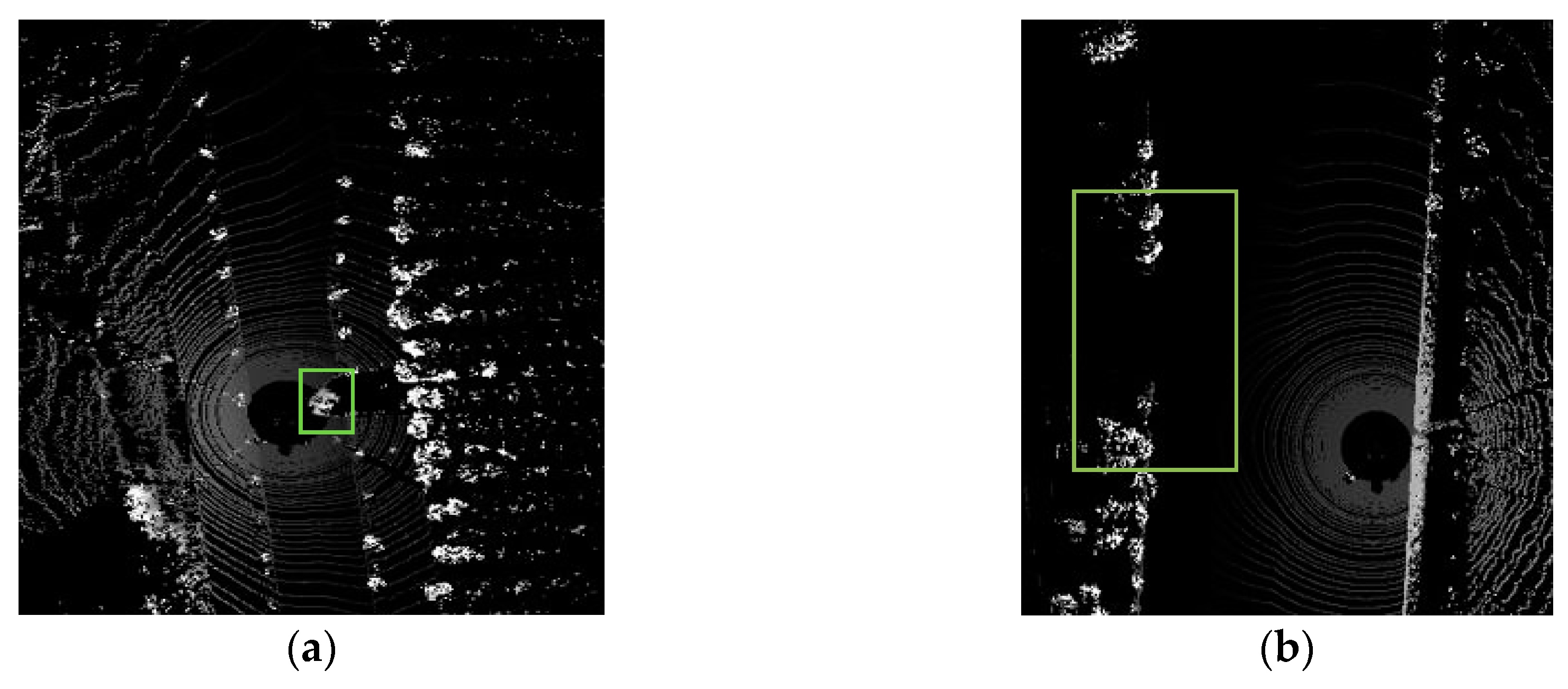
Two typical scenes are shown in Figure 10 to illustrate the difficulties in road curb detection. The green box in the left image shows that a car is parking on the roadside, which would be detected as a road curb if only the local information is applied. The green box in the right image shows that a gap exists between two segments of the road curb, and this gap would cause the leak detection of the road curb if only the local information is applied.
However, it is not difficult to learn the road’s overall shape information despite the existence of the obstacle inside the road area and the interval of the curb. The road’s overall shape information can be reflected by the road centerline, and the road width information. Besides, the real road width can be obtained by the road width distribution.
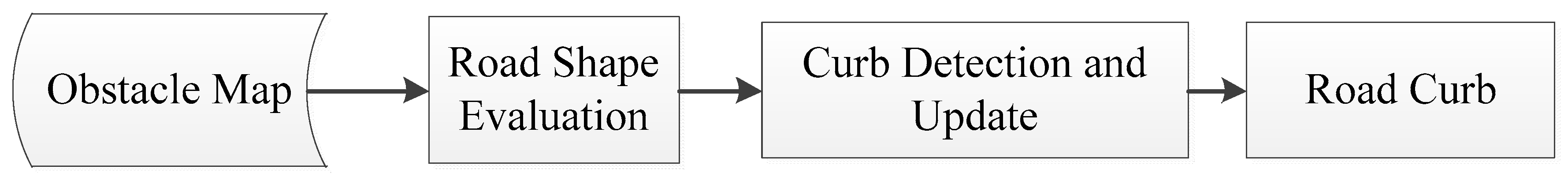
A road curb detection method based on the road’s overall shape information is presented in this section, and its flow diagram is shown in Figure 11.The method can be divided into two parts: road shape evaluation and curb detection and update.
3.1. Road Shape Evaluation
In this part, a two-step, centerline extraction and road width estimation, method is proposed to estimate the road shape.
3.1.1. Centerline Extraction
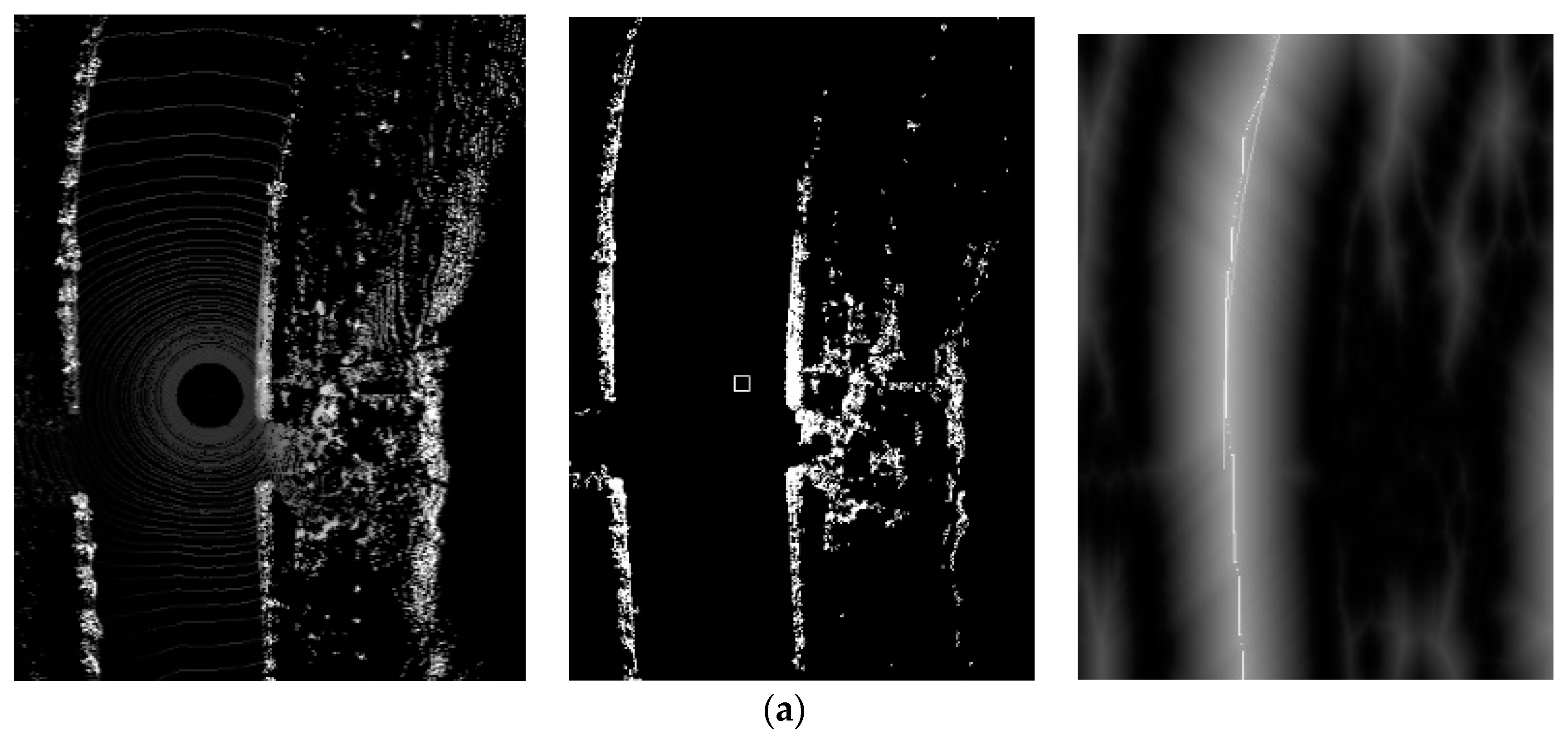
After the ground segmentation, a grid map that only contains two values is created, obstacles are marked as 0 and other grids are marked as 255. Each grid cell of the map represents 20 cm. Then a distance transformation, which uses Algorithm 1, is conducted and the grid intensity increases with the distance between the grid and an obstacle grid. An example of the distance transformation performed on the obstacle map is shown in Figure 12. As shown in Figure 12c, the intensities of the points in the road centerline is the local maximum because the distance between the points in the road centerline and its nearest obstacle point is the maximum compared with its local neighboring points. Moreover, the road centerline reflects the trend of the road.
| Algorithm 1. Distance Map Generation Process |
| Distance Transform Algorithm |
| Input: ObstacleMap |
| Input: MAP_WIDTH |
| Input: MAP_HEIGHT |
| Output: DistanceMap |
| Function Begin |
| PixelValueBinaryzation(OMap) |
| for i← 1 to MAP_HEIGHT − 2 |
| for j← 1 to MAP_WITH − 2 |
| DistanceMap [i + 1][j] = min(ObstacleMap [i][j] + 1, ObstacleMap [i + 1][j]) |
| DistanceMap [i + 1][j + 1] = min(ObstacleMap [i][j] + 1, ObstacleMap [i + 1][j + 1]) |
| DistanceMap [i][j + 1] = min(ObstacleMap [i][j] + 1, ObstacleMap [i][j + 1]) |
| DistanceMap [i − 1][j + 1] = min(ObstacleMap [i][j] + 1, ObstacleMap [i − 1][j + 1]) |
| end for |
| end for |
| for i← MAP_HEIGHT − 2 to 1 |
| for j← MAP_WITH − 2 to 1 |
| DistanceMap [i − 1][j] = min(ObstacleMap [i][j] + 1, ObstacleMap [i − 1][j]) |
| DistanceMap [i − 1][j − 1] = min(ObstacleMap [i][j] + 1, ObstacleMap [i − 1][j − 1]) |
| DistanceMap [i][j − 1] = min(ObstacleMap [i][j] + 1, ObstacleMap [i][j − 1]) |
| DistanceMap [i + 1][j − 1] = min(ObstacleMap [i][j] + 1, ObstacleMap [i + 1][j − 1]) |
| end for |
| end for |
| Function End |
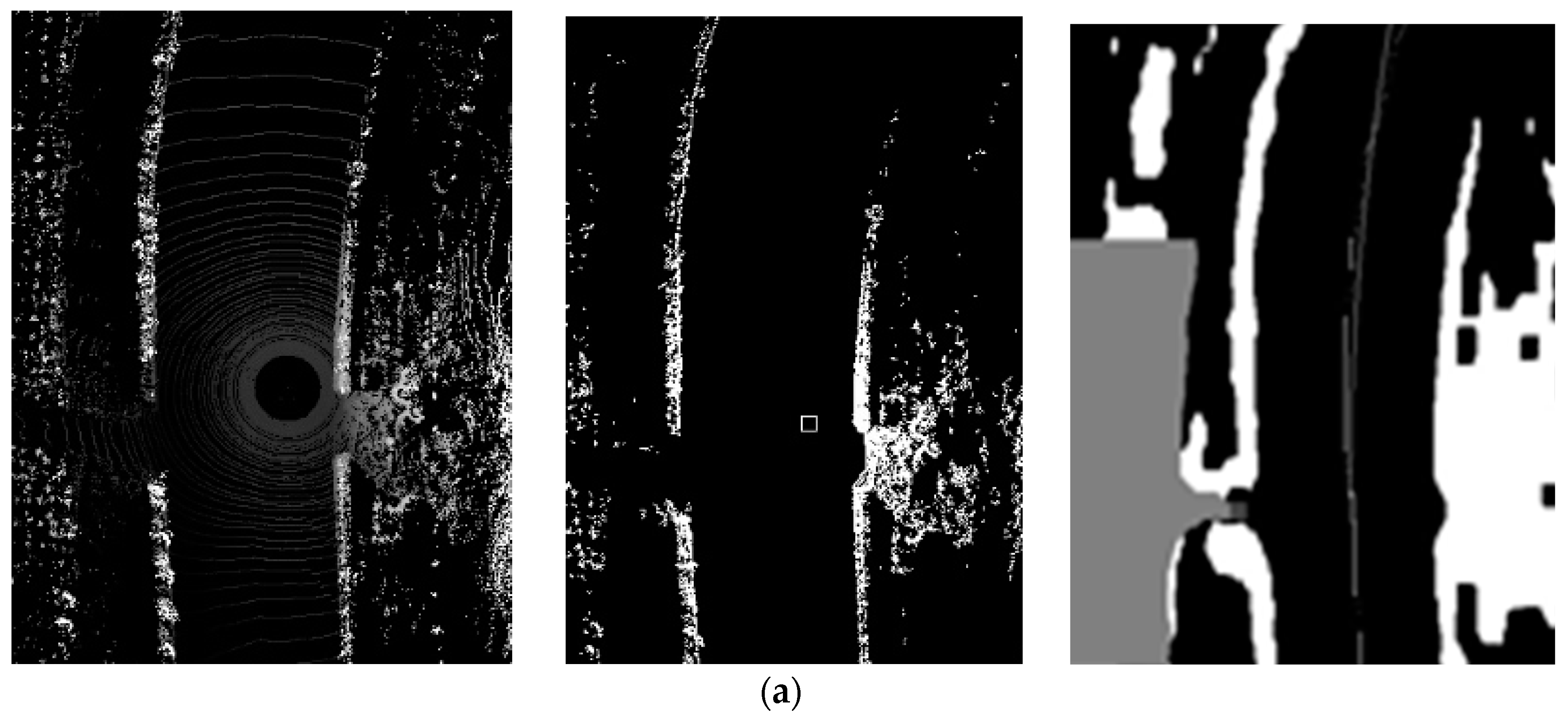
In most cases, the Lidar is not found in the road’s center position. Therefore, a seed point should be obtained to generate the entire road centerline. As shown in Figure 12c, the intensity in the distance map varies continuously, which means that the gradient information can be applied to find the nearest local maximum point. Search from the vehicle’s position to find the local maximum point in 5 × 5 model. The point is set as the seed point if it is the local maximum point in the 5 × 5 model centered on itself. Otherwise, the search is continued until a point is the local maximum point in the 5 × 5 model centered on itself. The result of obtaining the nearest local maximum point is shown in Figure 13, where the upper right box is the position of the Lidar, whereas the lower left box is the position of the nearest local maximum point.
Starting from the nearest local maximum position, a search is performed on the distance map to find the local maximum points in the upward and downward directions. This step is followed by quadratic curve fitting and the result is in the form of (5).
Figure 14a shows the extraction of the centerline in a winding road situation. The third column shows that the extracted centerline reflects the road trend. A situation where the distance map is affected by the obstacle inside the road area is shown in Figure 14b. It can be seen that the extracted centerline is not in the center position of the road area. The centerline should satisfy two requirements. First, the line should reflect the road trend generally. Second, the line should be found inside the road area. Our experiment found that these two requirements are relatively easy to meet if a relatively large model is selected to lead to the detection of a long centerline, for example a 10 × 10 model. A longer centerline detected inside the road area means a more accurate quadratic curve fit for the road shape. As shown in the green box in Figure 14b, the road centerline is continuous in the distance map despite the existence of the obstacle inside the road area. Thus, a long centerline inside the road area can be extracted.
3.1.2. Road Width Estimation
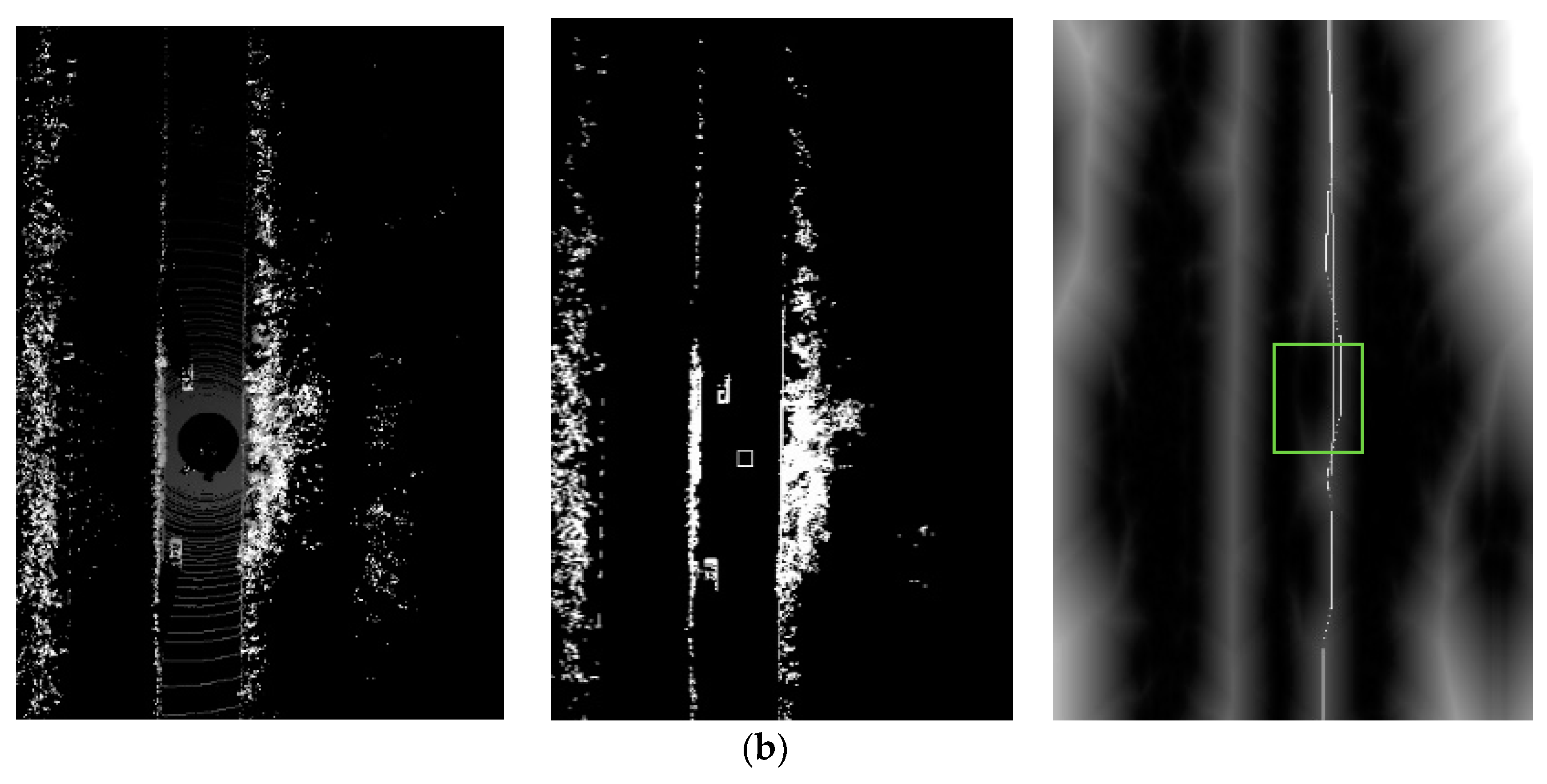
To increase the continuity of the obstacle map, instead of using a normally morphological close operation on the obstacle map, a threshold segmentation, which is less time consuming, is performed on the distance map. Pixels less than the threshold are set as 255 and the rest pixels are set as 0. The result is shown in Figure 15. Figure 15c shows that the road curb points are more continuous than the original obstacle map. Moreover, the road curb is smoother than the original obstacle map, and the high-frequency noise caused by the uneven sample is reduced.
Based on the aforementioned analysis, road trend and a more continuous obstacle map are obtained. Points in the road centerline, whose y value is in the interval of [STARTY, ENDY], are used as seed points and a search is performed from a seed point in left and right directions until an obstacle point is met. In this manner, the distances of the point to the left and the right nearest obstacles can be obtained. By summing these two distances up for each point in the road centerline, the road width distribution can be obtained. Based on statistics, the most likely width of the road can be obtained. The detailed algorithm is shown in Algorithm 2.
| Algorithm 2. Process for the Analysis of Width Distribution |
| RoadWidthAnalysis |
| RoadWidthCount[0]← {0} |
| maxWidthCount← 0 |
| For y← STARTY to ENDY |
| LeftWidth← 0 |
| While ThreSegImg[y][x − LeftWidth] == 0 |
| LeftWidth ++ |
| End While |
| RightWidth← 0 |
| While ThreSegImg[y][x + RightWidth] == 0 |
| RightWidth ++ |
| End While |
| RoadWidth[y]← LeftWidth + RightWidth |
| Save the Point (x, y) to WidthPoints[RoadWidth[y]/10] |
| RoadWidthCount[RoadWidth[y]/10] ++ |
| If(RoadWidthCount[RoadWidth[y]/10] > maxWidthCount) |
| maxWidthCount← RoadWidthCount[RoadWidth[y]/10] |
| MaxRoadWidthPortion = RoadWidth[y]/10; |
| End if |
| End For |
In Algorithm 2, a search is performed between STRARTY and ENDY to find obstacle points of the road edge on both sides of the centerline. All the width values are assigned to partitions with a difference of 2 m. Thus, the points corresponding to the most possible width, i.e., points in the largest partition, can be selected as the seed points.
Two typical scenes are shown in Figure 16, where the gray area in the third column shows the width distribution of the road. A winding road is shown in the first row. In spite of the curved shape of the road, the width distribution of the road is continuous. An obstacle inside the road area situation is shown in the second row. The third column shows that the width distribution is affected by two vehicles. However, based on the maximum possible width analysis, the true road width can be obtained. In this manner, the vehicle inside the road is not regarded as the road curb.
3.2. Curb Detection and Update
The seed points are applied to detect the entire road curb points by region growing in the original obstacle map. The candidate road curb points should satisfy the following criterion: the gradient in the x-direction should be negative for the left curb candidate road curb points while positive for the right curb candidate road curb points. Thereafter, a quadratic curve fitting is performed on the candidate points. The result is shown in Figure 17c.
As shown in the white box in the third column of the first row, a gap exits in the road curb. However, based on the width distribution information, seed points in the two sides of the road curb are obtained, and they are grown to obtain the road curb candidate points in the two sides of the gap. The white boxes in the third column of the first row show two vehicles. The partially enlarged detail map shows that the curb points between the upper vehicles are detected, whereas the curb points between the lower vehicles are leak-detected. This difference is caused by the difference in the gaps between the vehicles, such that the curb points in the left side of the lower vehicle are not regarded as the road curb points. However, this difference does not affect the extraction of the road curb because most road curb points are detected and the shape of the road curb is reflected.
Then, a multi-index evaluation of road curb in three aspects, including the shape of the road curb, the fit degree between the road curb and the scene, and the variance between the curve and history information, is presented in this study. These aspects are described in detail in the subsequent subsections.
3.2.1. Shape of the Road Curb
The shape of the road curb can be partially reflected by its curvature, which can be denoted by the coefficient of the fitted quadratic curve. The road trend changes relatively slowly in a local frame grabbed by Velodyne LIDAR. Thus, the coefficient of the quadratic curve should not exceed a certain threshold.
3.2.2. Fit Degree between the Road Curb and the Scene
The fit degree between the road curb and the scene reflects the property how the detected curve reflects the true shape of the road. This aspect is denoted by three indices in this study.
- The number of the detected curb points.
- The maximum difference of the y value between the detected points.
- The variance of the width distribution
Our experiment found that, if the number of the detected road curb points is excessively small, the points cannot reflect the shape of the road curb. Moreover, the more divergent these points are, the more accurate these points will reflect the road shape. The dispersion of the curb points can be reflected by their maximum difference of the y value. As the road is continuous, the road width distributions along the y-direction should be similar. Thus, the variance of the width distribution should be small.
3.2.3. Variance between the Curve and History Information
During driving, the road curb should be continuous in most cases. Thus, the curb shape between two consecutive frames should not change significantly. The consecutiveness of the road curb is denoted by the difference of the road width between two consecutive frames. The difference should not exceed a certain threshold, which is defined and tested with a lot of experiments conducted on our autonomous vehicle.
In our experiments, the position of the Lidar is (250, 500) in the grid map. Each cell represents 20 cm. As the obstacle information is more detailed near the Lidar, STARTY is set as 100 and ENDY is set as 400 in our experiment. The thresholds selected for the aforementioned indices are shown in Table 2.
The prediction and update of the road curb are described in detail in [24], which predict the initial position of the road curb of this frame based on the motion of the vehicle from the previous curb position and the update of the height difference map generated by this frame data using SNAKE Model.
4. Experimental Results and Discussion
Our experimental platform is the autonomous vehicle named “Intellgent Pioneer”, as shown in Figure 2. Besides three-dimensional Lidar, it is equipped with a SPAN-CPT, an integrated navigation device combining inertial navigation and Global Positioning System, which provides accurate position and moving state of the intelligent vehicle.
To validate the robustness and accuracy of the ground segmentation algorithm presented in this work, experiments under various environments are conducted including straight road, winding road and crossroad in urban area and off-road area. Figure 18a shows the heavy traffic situation. The existence of the obstacle influences the local geometric characteristics of the tangential neighboring points on the ground, which would be falsely detected based on some features alone. The four features are fused in different scopes and the ground segmentation is completely without over segmentation. Figure 18b shows ground segmentation with a low irregular obstacle inside the road area. As shown in the real scene picture, three rows of cones are in front of the intelligent vehicle, which were low and difficult to detect. The detection of a negative obstacle is shown in Figure 18c, where two pits exist in the scene. A round pit and a rectangular pit are marked out in the red box in the second row. As shown in the figure, with the ground cleanly segmented, the points projected on the round pit are mostly detected as obstacles, and several points projected onto the rectangular pit are detected as obstacles.
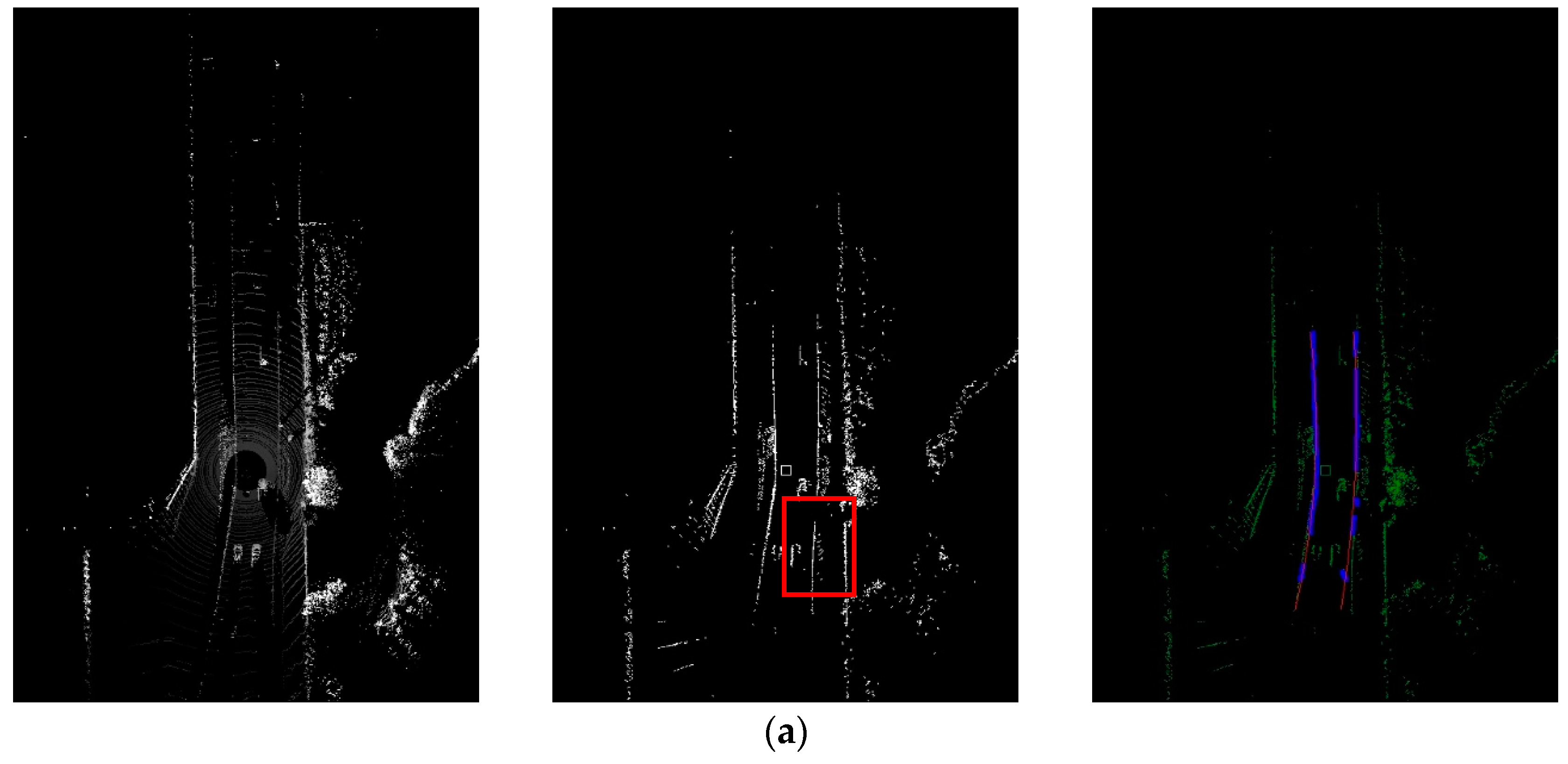
The comparison between the proposed ground segmentation method and that of [23] is presented in Figure 19, where a low stone curb situation is shown. The result of the ground segmentation algorithm presented in [23] is shown in Figure 19b, whereas the result of this study is shown in Figure 19c. According to the gradient feature presented in [23], although the curb points near the vehicle have been detected continuously, the curb points distant from the vehicle were leak-detected. As mentioned previously, when the curb points detected are more divergent, the curb shape is reflected to be more accurate. Figure 19c shows that the curb detected by the algorithm presented in this study covered a broader scope despite the existence of gaps, which shows more information on the road trend.
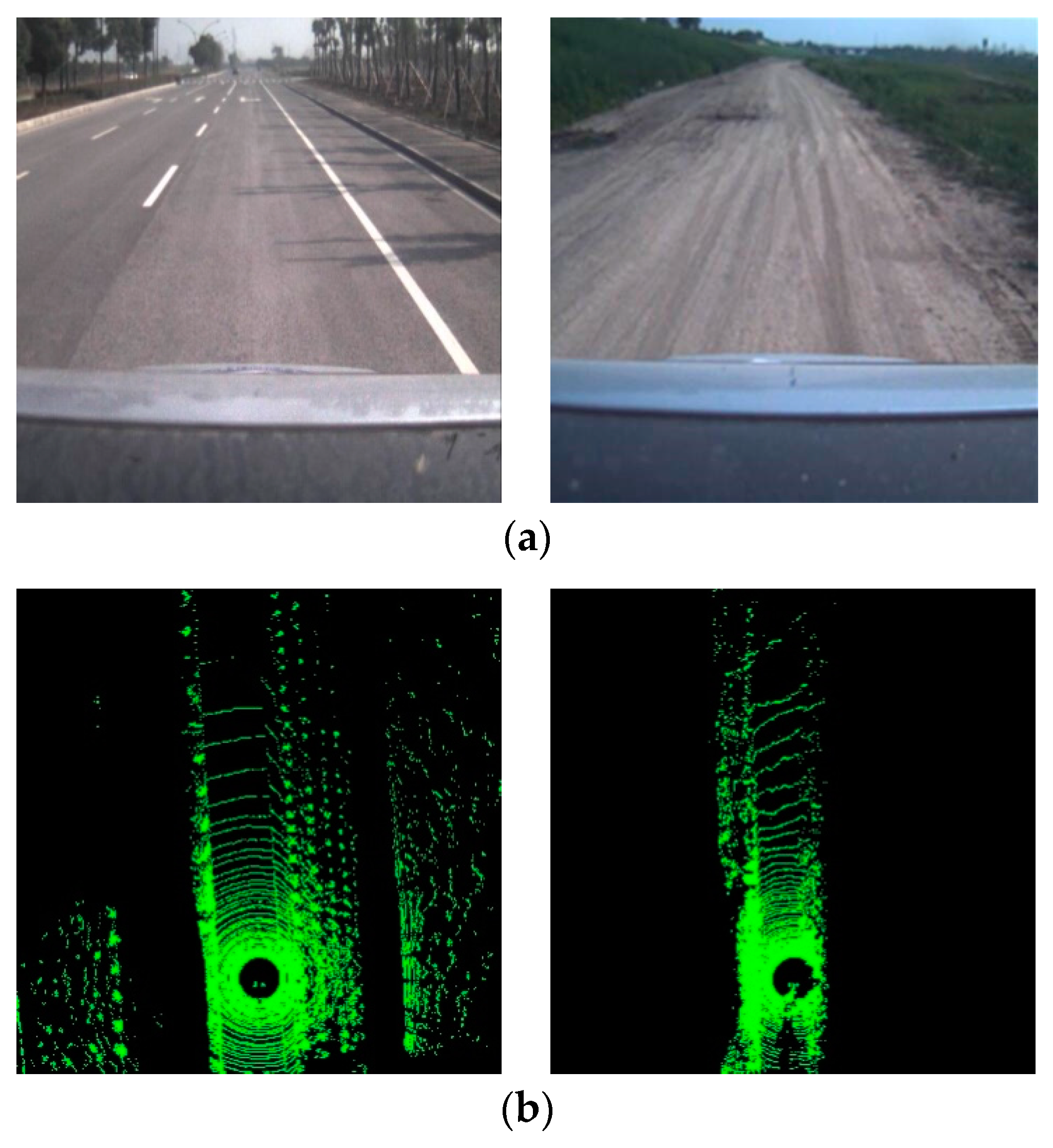
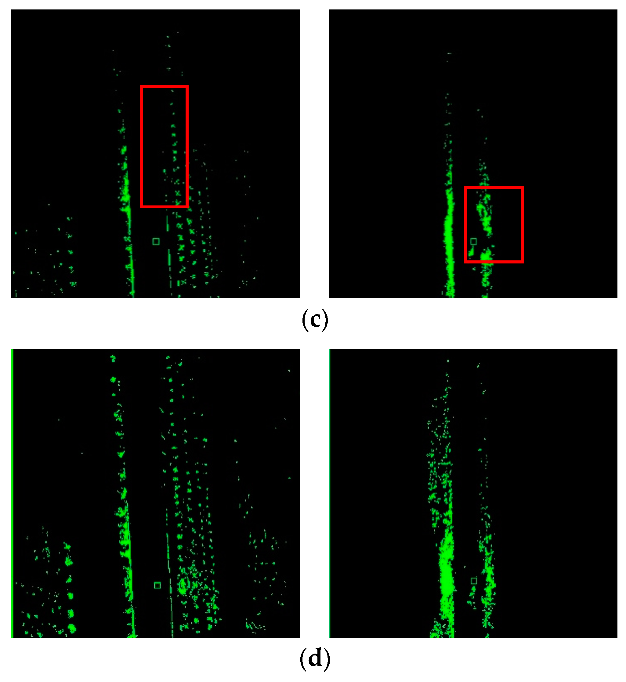
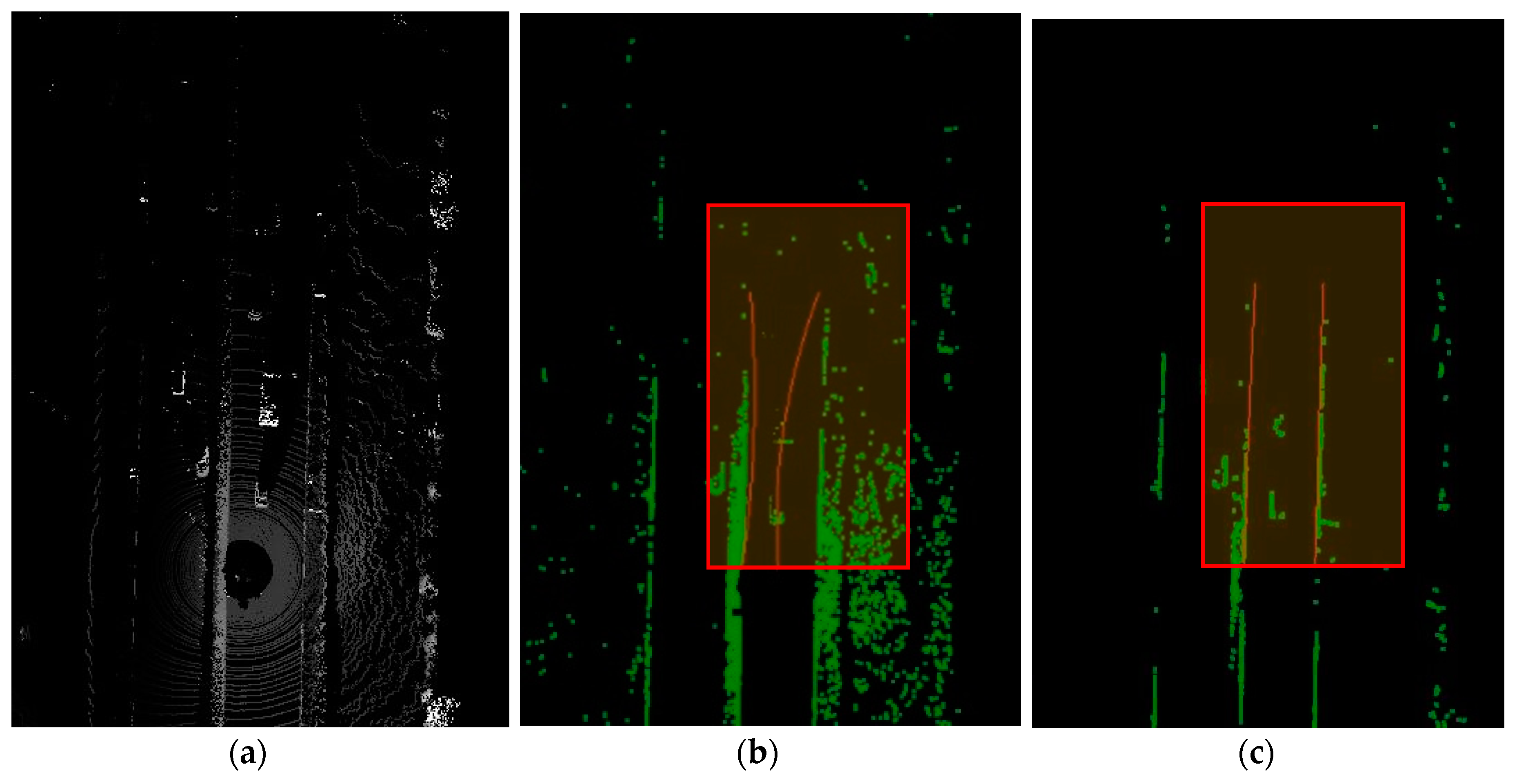
The comparison between the ground segmentation of this study and that of [24] is presented in Figure 20, which contains the real scene image, yaw point cloud, result obtained by the algorithm presented in [24], and result obtained by the algorithm presented in this study. The experiment found that the distance based features are insensitive to the influence exerted by the distant obstacles on the local geometric characteristic. Whereas, the angle based features are insensitive to the influence exerted by the nearby obstacles. Global thresholds are applied in [24] to segment the ground. Therefore, leak detection is inevitable as shown in the red box in Figure 20c. As an in-depth analysis is performed on the threshold and the fitted scope of each feature applied in this study, leak detection is reduced compared with the algorithm presented in [24], as shown in Figure 20d.
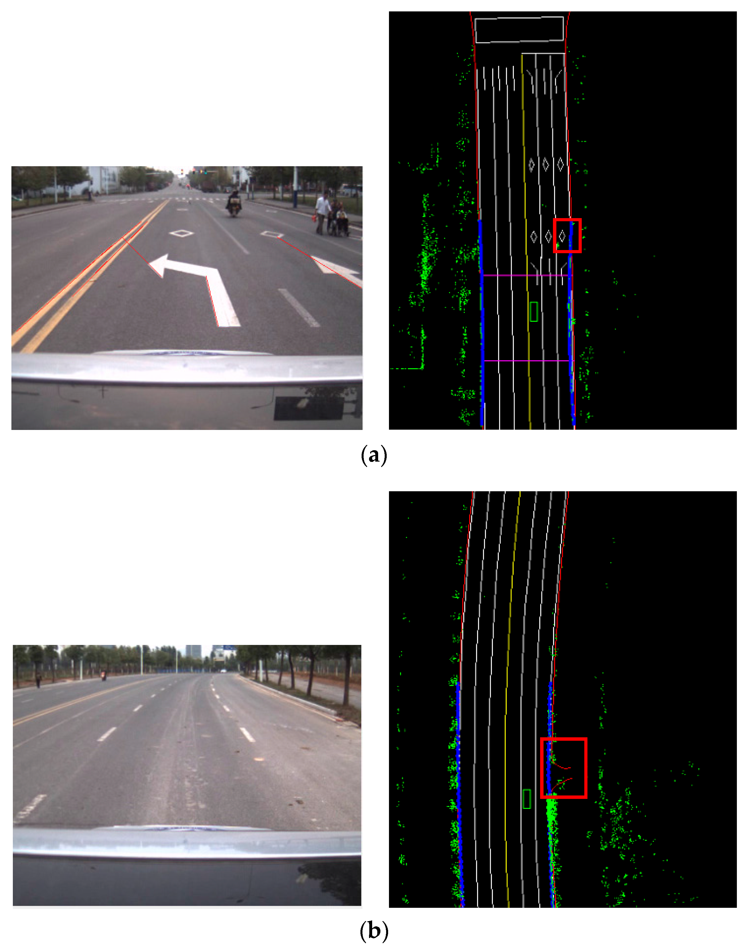
The result of road curb detection in the three scenes are shown in Figure 21, including the yaw point cloud, obstacle map, and detected road curb, respectively. A common difficulty for road curb detection in these scenes is the existence of the obstacle inside the road area, which may influence the detection of the road curb.
Figure 21a shows an urban scene where the road width varied and the number of vehicles inside the road generated interference on road curb detection. Based on the analysis of the road’s overall trend information, the vehicles inside the road were identified as dynamic obstacles instead of the road curb. Moreover, the existence of the dynamic obstacles inside the road area caused the leak detection of the low curb, as shown in the red box in the second column, which did not affect the detection of the road curb. Figure 21b shows the influence of snowy weather on road curb detection. As shown in the first column, the noise points on the road are generated by the snow. However, the road curb was correctly detected without being influenced by these noise points. A field scene is shown in Figure 21c, where the coarse ground in the left of the vehicle was detected as an obstacle. Moreover, the curb is rough. The detection results shown in the third column shows that the curb was correctly detected.
The comparison between the results of road detection in [24] and that in this study is shown in Figure 22. The result of [24] is shown in Figure 22b and the obstacle inside the road was detected as a road curb as the lack of the road’s overall information. The result of this study is shown in Figure 22c. As the road’s overall information was applied in this work, the obstacle inside the road was not designated as the road curb.
The results of an experiment measuring the time needed for road curb detection are shown in Figure 23 where the blue line shows the time consumption based on detection solely and the yellow line shows the time consumption based on the framework presented in this study. The average time of the detection solely method is 112 ms and the peak value is larger than 900 ms as a result of the limit of the multi-threaded framework used in the program. The proposed framework is much faster, the average time is 11 ms, and the value is stable.
To evaluate the accuracy of the proposed curb detection method, a comparison between the detection result and the road curb in a high precision map is conducted. The testing path is shown in Figure 24 with red lines. The blue lines are lane marks in the map. The path is about 9.2 km including 4.9 km straight road and 4.3 km winding road.
The curbs in high precision map can be treated as ground truth whose error is less than 10 cm. To reduce the impact of positioning errors RTK differential positioning system is used and the positioning error is less than 5 cm. Distance between the detected curbs and the ground truth can be worked out in the local coordinate of the intelligent vehicle. The intelligent vehicle is moving along the road and the horizontal distance between a detection curb point and the ground truth point with the same vertical coordinate can be obtained as the curb detection error. The accuracy of the proposed method and method of [24] is shown in Table 3. The average detection error of our method is smaller than method of [24] on both straight road and winding road. Besides, the accuracy difference of the proposed method between on straight road and on winding road is smaller, which demonstrates a better robustness.
Two typical scenes on straight road and winding road are shown in Figure 25. Red lines are road curbs in high precision map and blue lines are detected road curbs. The proposed method is robust to obstacles on road and discontinuity of road curbs which are shown in red boxes. The detected results are consistent with the ground truth.
5. Conclusions
This paper introduced a quick and accurate method for online road curb detection using multi-beam Lidar. In the process of ground segmentation, a multi-feature, loose threshold, varied-scope method is used to increase the robustness. Then, an extraction-update mechanism based road curb detection method is proposed and the overall road shape information is used in the extraction process.
Experimental results show that the proposed ground segmentation method performs much better than the method in [23] and the method in [24]. The robustness is proved by applying the method in different scenes including congested viaduct, urban road with obstacles at night and road with negative obstacles. Besides, the road curb detection method is 10 times faster than the detection solely method and the detection speed is stable. The accuracy is also evaluated and it is sufficient for autonomous driving.
Our future work will focus on improving the accuracy and rationality of thresholds used in ground segmentation and maybe an adaptive method will be adopted according to the road roughness. Another research direction is the fusion of data from Lidar and camera to increase the robustness and accuracy of curb detection.
Acknowledgments
We would like to acknowledge all of our team members, whose contributions were essential for this paper. We would also like to acknowledge the support of National Nature Science Foundations of China (Grant No. 61503362, 61305111, 61304100, 51405471, 61503363, 91420104), National Science Foundation of Anhui Province (Grant No. 1508085MF133, KJ2016A233)
Author Contributions
All six authors contributed to this work. Rulin Huang and Jian Liu were responsible for the literature search algorithm design and data analysis. Jiajia Chen, Biao Yu, Lu Liu and Yihua Wu made substantial contributions to the planning and design of the experiments. Rulin Huang was responsible for the writing of the paper and modified the paper. Finally, all of the listed authors approved the final manuscript.
Conflicts of Interest
The authors declare no conflict of interest.
References
- Dollar, P.; Wojek, C.; Schiele, B.; Perona, P. Pedestrian Detection: An Evaluation of the State of the Art. IEEE Trans. Pattern Anal. Mach. Intell. 2012, 34, 743–761. [Google Scholar] [CrossRef] [PubMed]
- Shu, Y.; Tan, Z. Vision based lane detection in autonomous vehicle. Intell. Control Autom. 2004, 6, 5258–5260. [Google Scholar]
- Bertozzi, M.; Broggi, A.; Cellario, M. Artificial vision in road vehicles. Proc. IEEE 2002, 90, 1258–1271. [Google Scholar] [CrossRef]
- Wen, X.; Shao, L.; Xue, Y. A rapid learning algorithm for vehicle classification. Inf. Sci. 2015, 295, 395–406. [Google Scholar] [CrossRef]
- Sivaraman, S.; Trivedi, M.M. A General Active-Learning Framework for On-Road Vehicle Recognition and Tracking. IEEE Trans. Intell. Transp. Syst. 2010, 11, 267–276. [Google Scholar] [CrossRef]
- Arrospide, J.; Salgado, L.; Marinas, J. HOG-Like Gradient-Based Descriptor for Visual Vehicle Detection. IEEE Intell. Veh. Symp. 2012. [Google Scholar] [CrossRef]
- Sun, Z.H.; Bebis, G.; Miller, R. On-road vehicle detection: A review. IEEE Trans. Pattern Anal. Mach. Intell. 2006, 28, 694–711. [Google Scholar] [PubMed]
- Huang, J.; Liang, H.; Wang, Z.; Mei, T.; Song, Y. Robust lane marking detection under different road conditions. In Proceedings of the 2013 IEEE International Conference on Robotics and Biomimetics, Shenzhen, China, 12–14 December 2013; pp. 1753–1758. [Google Scholar]
- Bengler, K.; Dietmayer, K.; Farber, B.; Maurer, M.; Stiller, C.; Winner, H. Three decades of driver assistance systems: Review and future perspectives. IEEE Intell. Trans. Syst. Mag. 2014, 6, 6–22. [Google Scholar] [CrossRef]
- Buehler, M.; Iagnemma, K.; Singh, S. The 2005 DARPA Grand Challenge; Springer: Berlin, Germany, 2007. [Google Scholar]
- Buehler, M.; Iagnemma, K.; Singh, S. The DARPA Urban Challenge; Springer: Berlin, Germany, 2009. [Google Scholar]
- Baidu Leads China’s Self-Driving Charge in Silicon Valley. Available online: http://www.reuters.com/article/us-autos-baidu-idUSKBN19L1KK (accessed on 22 July 2017).
- Ford Promises Fleets of Driverless Cars within Five Years. Available online: https://www.nytimes.com/2016/08/17/business/ford-promises-fleets-of-driverless-cars-within-five-years.html (accessed on 22 July 2017).
- What Self-Driving Cars See. Available online: https://www.nytimes.com/2017/05/25/automobiles/wheels/lidar-self-driving-cars.html (accessed on 22 July 2017).
- Uber Engineer Barred from Work on Key Self-Driving Technology, Judge Says. Available online: https://www.nytimes.com/2017/05/15/technology/uber-self-driving-lawsuit-waymo.html (accessed on 22 July 2017).
- Brehar, R.; Vancea, C.; Nedevschi, S. Pedestrian Detection in Infrared Images Using Aggregated Channel Features. In Proceedings of the 2014 IEEE International Conference on Intelligent Computer Communication and Processing, Cluj Napoca, Romania, 4–6 September 2014; pp. 127–132. [Google Scholar]
- Von Hundelshausen, F.; Himmelsbach, M.; Hecker, F.; Mueller, A.; Wuensche, H.-J. Driving with Tentacles: Integral Structures for Sensing and Motion. J. Field Robot 2008, 25, 640–673. [Google Scholar] [CrossRef]
- Urmson, C.; Anhalt, J.; Bagnell, D.; Baker, C.; Bittner, R.; Clark, M.N.; Dolan, J.; Duggins, D.; Galatali, T.; Geyer, C.; et al. Autonomous Driving in Urban Environments: Boss and the Urban Challenge. J. Field Robot 2008, 25, 425–466. [Google Scholar] [CrossRef]
- Kammel, S.; Ziegler, J.; Pitzer, B.; Werling, M.; Gindele, T.; Jagzent, D.; Schroder, J.; Thuy, M.; Goebl, M.; von Hundelshausen, F.; et al. Team AnnieWAY’s Autonomous System for the 2007 DARPA Urban Challenge. J. Field Robot 2008, 25, 615–639. [Google Scholar] [CrossRef]
- Montemerlo, M.; Becker, J.; Bhat, S.; Dahlkamp, H.; Dolgov, D.; Ettinger, S.; Haehnel, D.; Hilden, T.; Hoffmann, G.; Huhnke, B.; et al. Junior: The Stanford Entry in the Urban Challenge. J. Field Robot 2008, 25, 569–597. [Google Scholar] [CrossRef]
- Thrun, S.; Montemerlo, M.; Dahlkamp, H.; Stavens, D.; Aron, A.; Diebel, J.; Fong, P.; Gale, J.; Halpenny, M.; Hoffmann, G.; et al. Stanley: The Robot that Won the DARPA Grand Challenge. J. Field Robot 2006, 23, 661–692. [Google Scholar] [CrossRef]
- Moosmann, F.; Pink, O.; Stiller, C. Segmentation of 3D Lidar Data in Non-Flat Urban Environments Using a Local Convexity Criterion. In Proceedings of the 2009 IEEE Intelligent Vehicles Symposium, Xi’an, China, 3–5 June 2009; pp. 215–220. [Google Scholar]
- Cheng, J.; Xiang, Z.; Cao, T.; Liu, J. Robust vehicle detection using 3D Lidar under complex urban environment. In Proceedings of the 2014 IEEE International Conference on Robotics and Automation, Hong Kong, China, 31 May–7 June 2014; pp. 691–696. [Google Scholar]
- Liu, J.; Liang, H.; Wang, Z.; Chen, X. A Framework for Applying Point Clouds Grabbed by Multi-Beam LIDAR in Perceiving the Driving Environment. Sensors 2015, 15, 21931–21956. [Google Scholar] [CrossRef] [PubMed]
- Chen, T.; Dai, B.; Liu, D.; Song, J.; Liu, Z. Velodyne-based curb detection up to 50 meters away. In Proceedings of the 2015 IEEE Intelligent Vehicles Symposium, Seoul, South Korea, 28 June–1 July 2015; pp. 241–248. [Google Scholar]
- Zhao, G.; Yuan, J. Curb detection and tracking using 3D-LIDAR scanner. In Proceedings of the 19th IEEE International Conference on Image Processing, Orlando, FL, USA, 30 September–3 October 2012; pp. 437–440. [Google Scholar]
- Hata, A.Y.; Osorio, F.S.; Wolf, D.F. Robust Curb Detection and Vehicle Localization in Urban Environments. In Proceedings of the 2014 IEEE Intelligent Vehicles Symposium, Dearborn, MI, USA, 8–11 June 2014; pp. 1264–1269. [Google Scholar]
- Zhang, Y.; Wang, J.; Wang, X.; Li, C.; Wang, L. A real-time curb detection and tracking method for UGVs by using a 3D-LIDAR sensor. In Proceedings of the IEEE Conference on Control Applications, Sydney, Australia, 21–23 September 2015; pp. 1020–1025. [Google Scholar]
Figure 1.
Framework for road curb detection and tracking.

Figure 2.
System introduction. (a) Intelligent Pioneer; (b) Raw point cloud; (c) Local coordinate.

Figure 3.
Schematic figure of obstacle scanning.

Figure 4.
Result of projecting a typical driving scene onto the horizontal plane. (a) Real scene picture; (b) Grid map of yaw point cloud; (c) Partially enlarged detail map.
Figure 4.
Result of projecting a typical driving scene onto the horizontal plane. (a) Real scene picture; (b) Grid map of yaw point cloud; (c) Partially enlarged detail map.
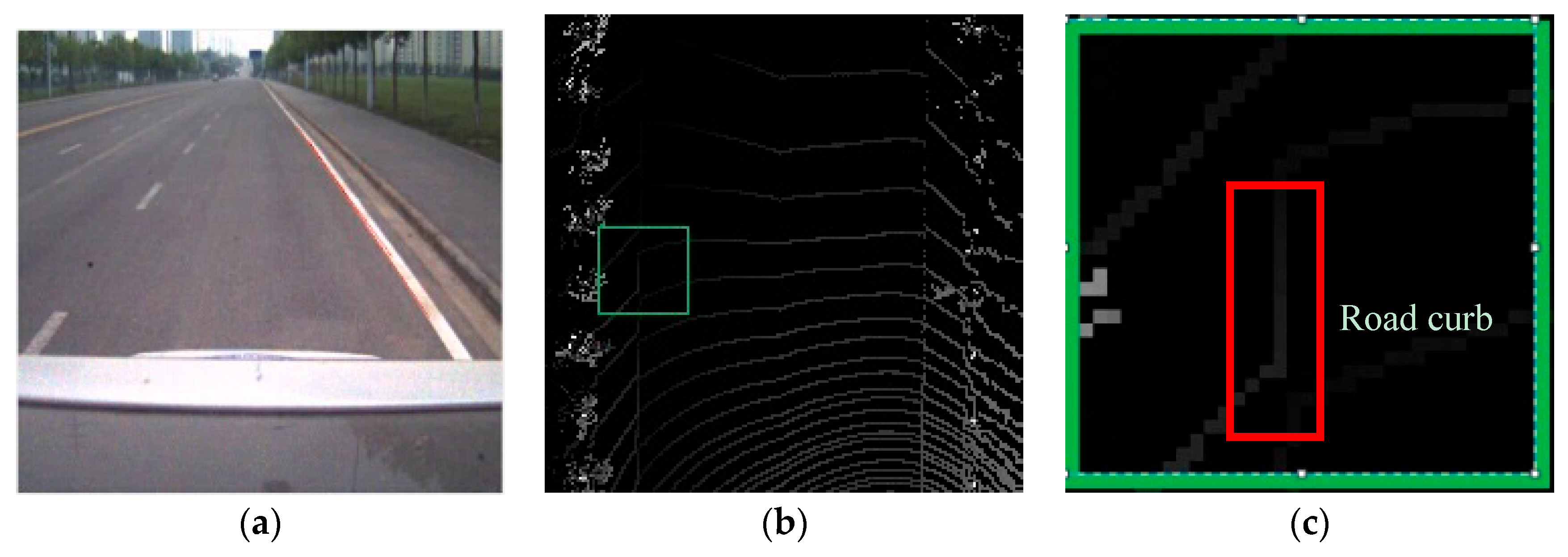
Figure 5.
Schematic diagram for the construction of the tangential angle. (a) Map of original point cloud; (b) Schematic diagram.
Figure 5.
Schematic diagram for the construction of the tangential angle. (a) Map of original point cloud; (b) Schematic diagram.

Figure 6.
Schematic diagram for the variations between tangential angle and obstacle position.

Figure 7.
Schematic diagram for height difference based on the prediction of the radial gradient.
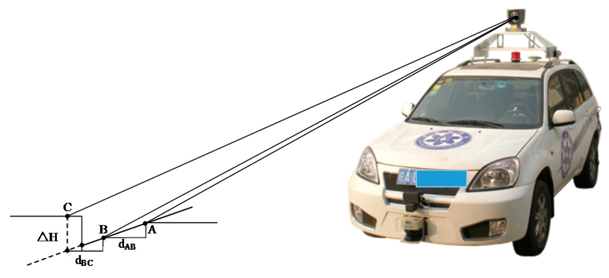
Figure 8.
Value distribution of the four features in a crossroad. (a) Maximum height difference in one grid; (b) Tangential angle feature; (c) Distance change between neighboring points in one spin; (d) Height difference based on the prediction of the radial gradient.
Figure 8.
Value distribution of the four features in a crossroad. (a) Maximum height difference in one grid; (b) Tangential angle feature; (c) Distance change between neighboring points in one spin; (d) Height difference based on the prediction of the radial gradient.
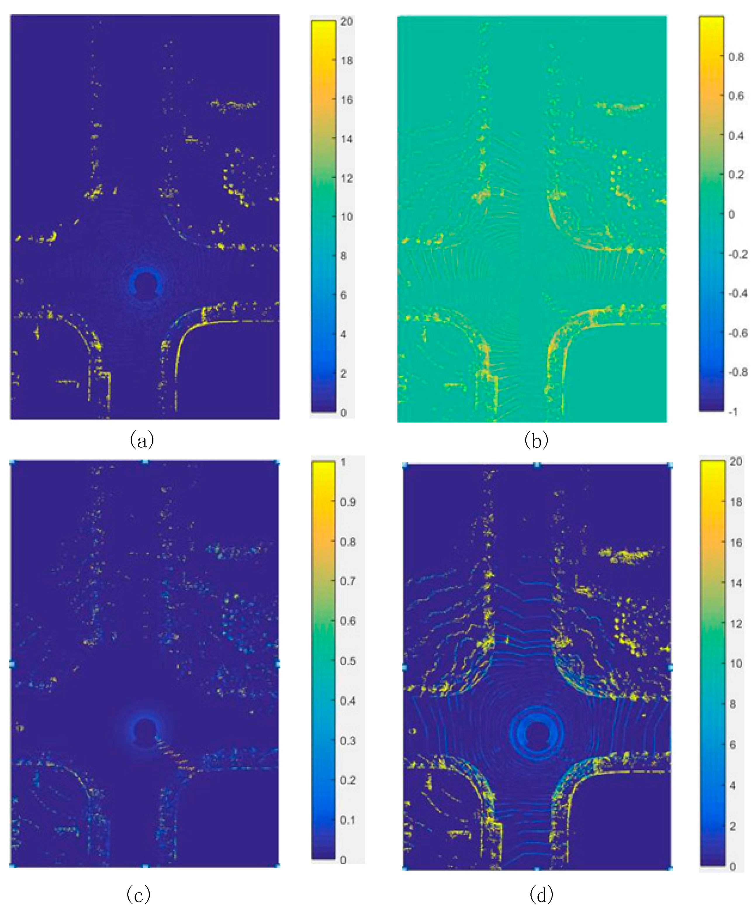
Figure 9.
Schematic diagram for the influence of the obstacle on its tangential neighboring point.

Figure 10.
Two typical scenes illustrating the difficulties for road curb detection. (a) A car parking inside the road; (b) A gap exists in the road curb.
Figure 10.
Two typical scenes illustrating the difficulties for road curb detection. (a) A car parking inside the road; (b) A gap exists in the road curb.

Figure 11.
Road curb extraction diagram.

Figure 12.
Generation of the distance map. (a) Original point cloud map; (b) Obstacle map; (c) Distance intensity map.
Figure 12.
Generation of the distance map. (a) Original point cloud map; (b) Obstacle map; (c) Distance intensity map.
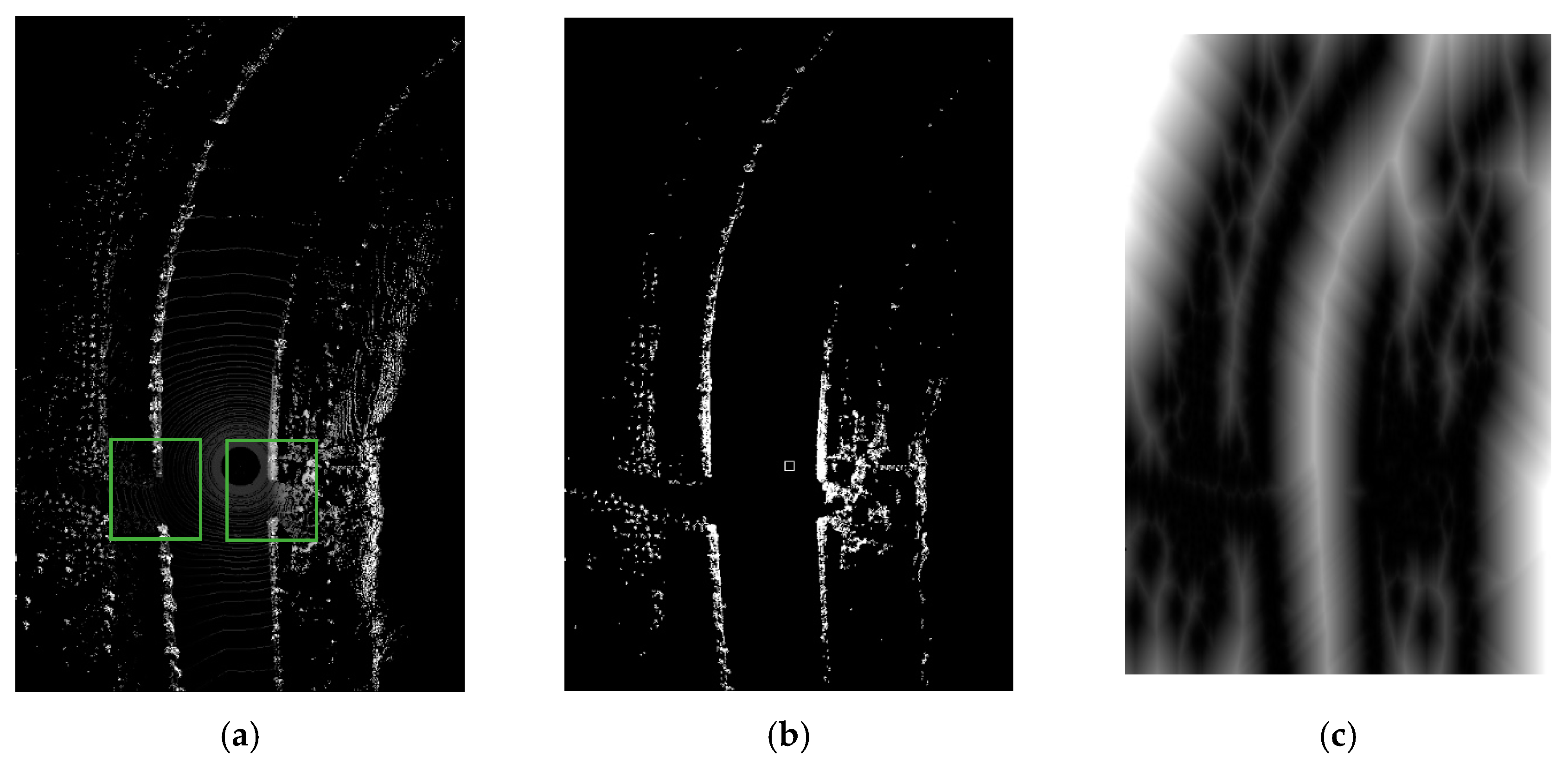
Figure 13.
Result of obtaining the nearest local maximum point. (a) Raw point cloud map; (b) Obstacle map; (c) Distance map.
Figure 13.
Result of obtaining the nearest local maximum point. (a) Raw point cloud map; (b) Obstacle map; (c) Distance map.
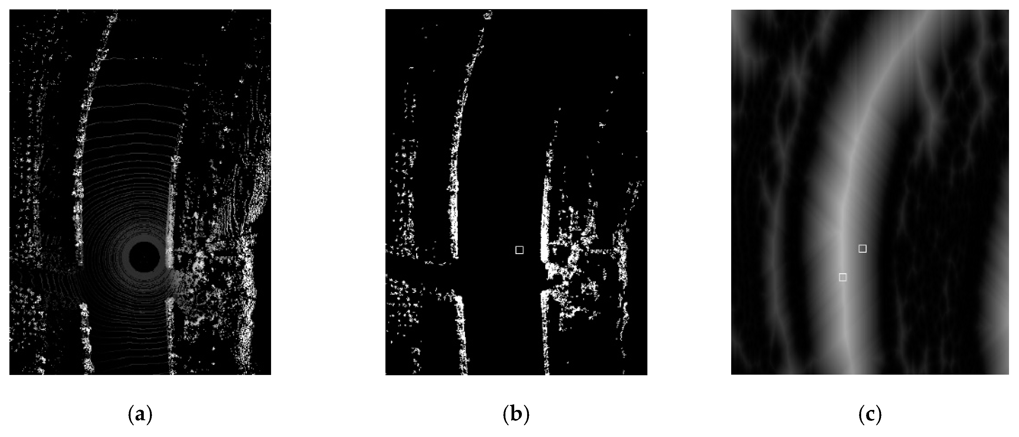
Figure 14.
Results for road centerline extraction of a winding road and a straight road. (a) Centerline extraction for winding road; (b) Centerline extraction for winding road.
Figure 14.
Results for road centerline extraction of a winding road and a straight road. (a) Centerline extraction for winding road; (b) Centerline extraction for winding road.


Figure 15.
Result of the threshold segmentation. (a) Original point cloud; (b) Obstacle map; (c) Segmentation result.
Figure 15.
Result of the threshold segmentation. (a) Original point cloud; (b) Obstacle map; (c) Segmentation result.
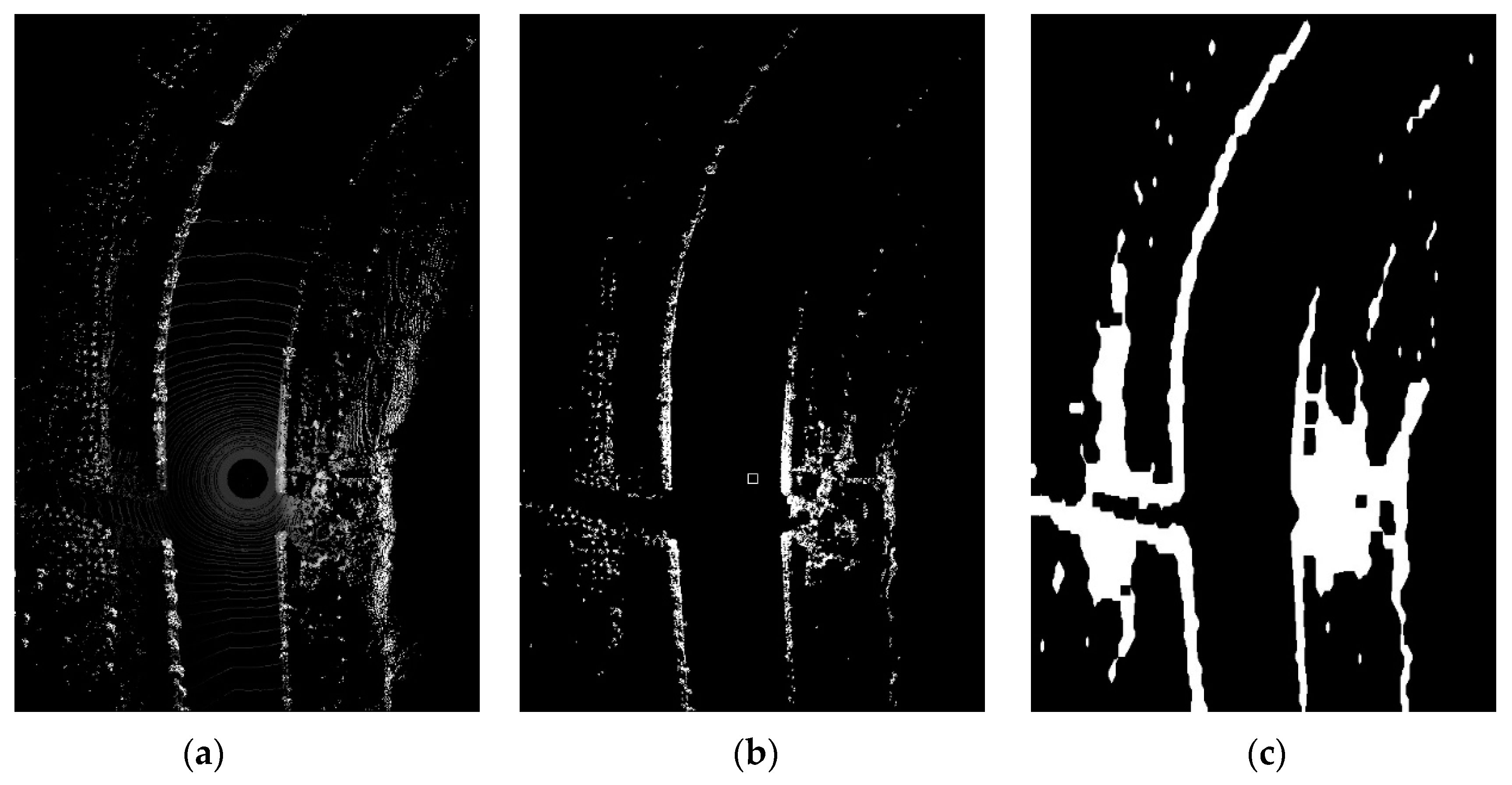
Figure 16.
Result of the width distribution in two typical scenes. (a) Width distribution of a winding road; (b) Width distribution of a straight road.
Figure 16.
Result of the width distribution in two typical scenes. (a) Width distribution of a winding road; (b) Width distribution of a straight road.

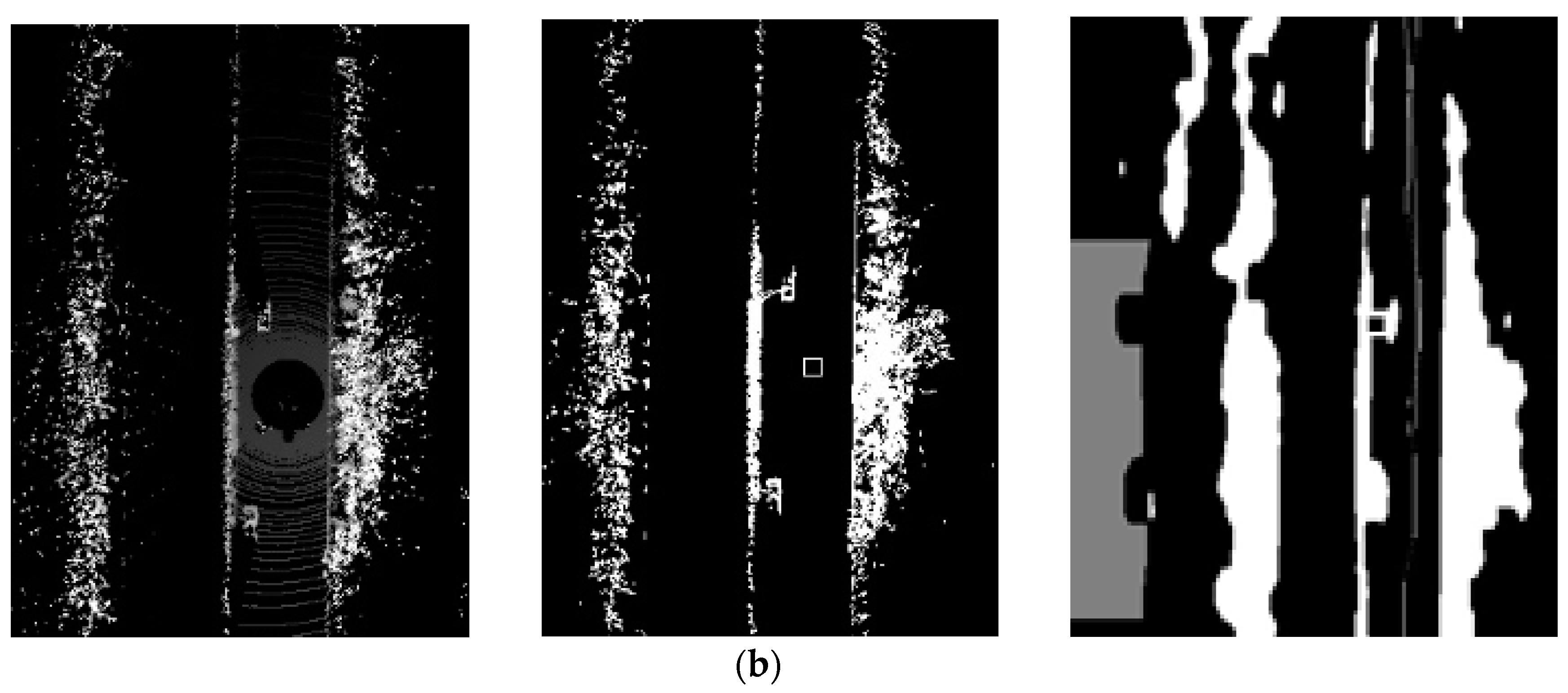
Figure 17.
Result of the region growing and curve fitting. (a) Obstacle map; (b) Width distribution; (c) Curve fitting result.
Figure 17.
Result of the region growing and curve fitting. (a) Obstacle map; (b) Width distribution; (c) Curve fitting result.

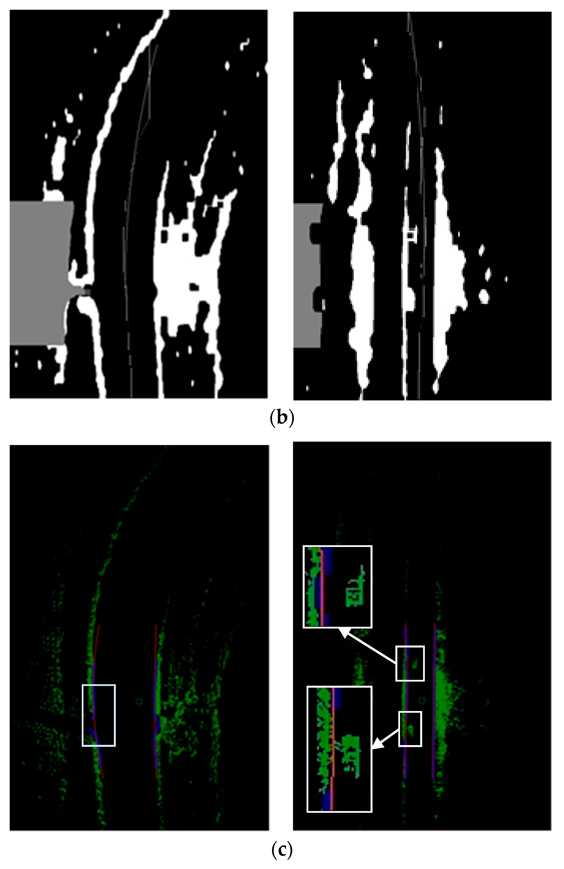
Figure 18.
Ground segmentation under various environments. (a) Congested viaduct; (b) Urban road with obstacles; (c) Off-road scene with negative obstacles.
Figure 18.
Ground segmentation under various environments. (a) Congested viaduct; (b) Urban road with obstacles; (c) Off-road scene with negative obstacles.
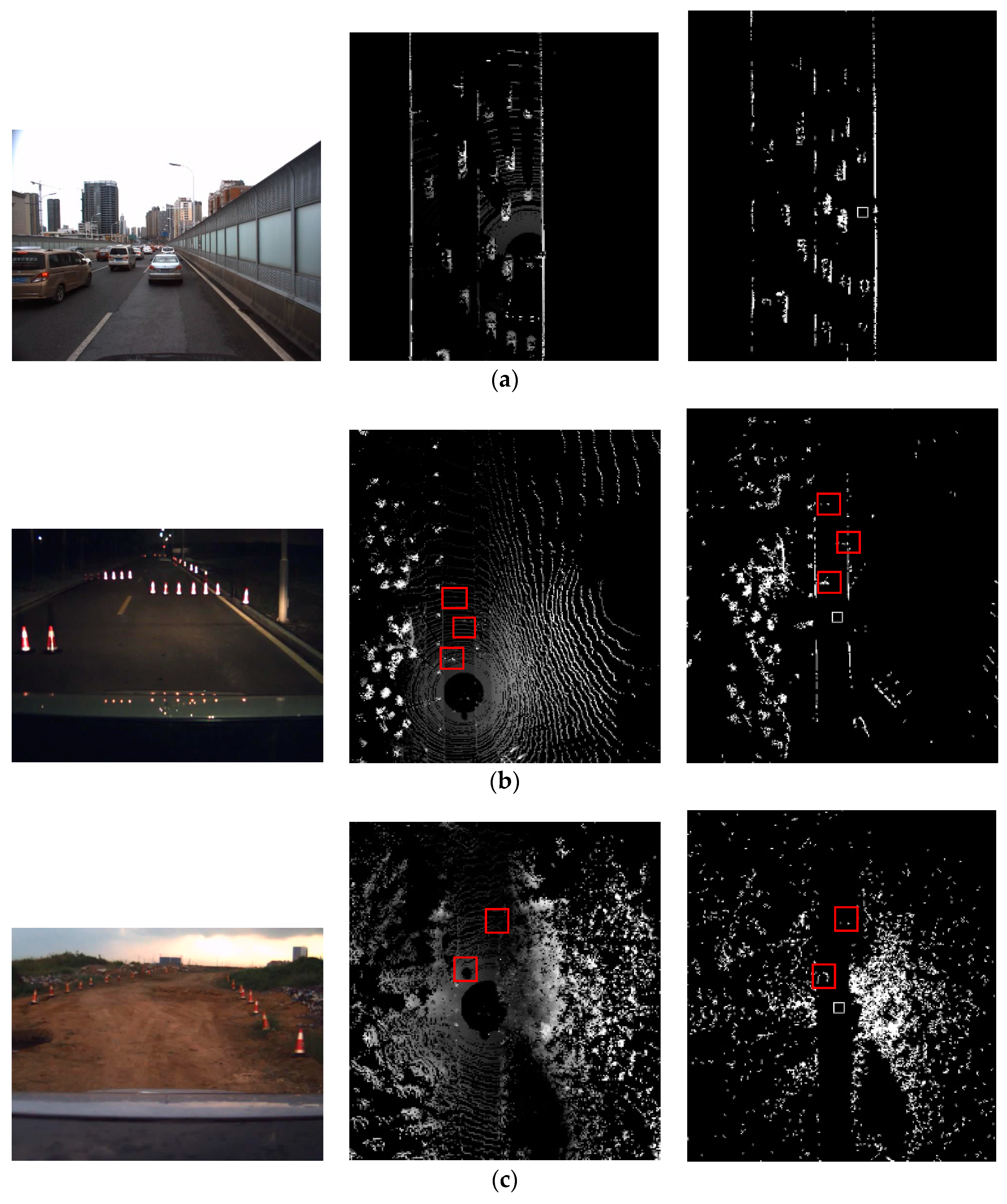
Figure 19.
Comparison of the ground segmentation method used in [23] and the proposed method. (a) Original point cloud map; (b) Result of the method used in [23]; (c) Result of the proposed method.
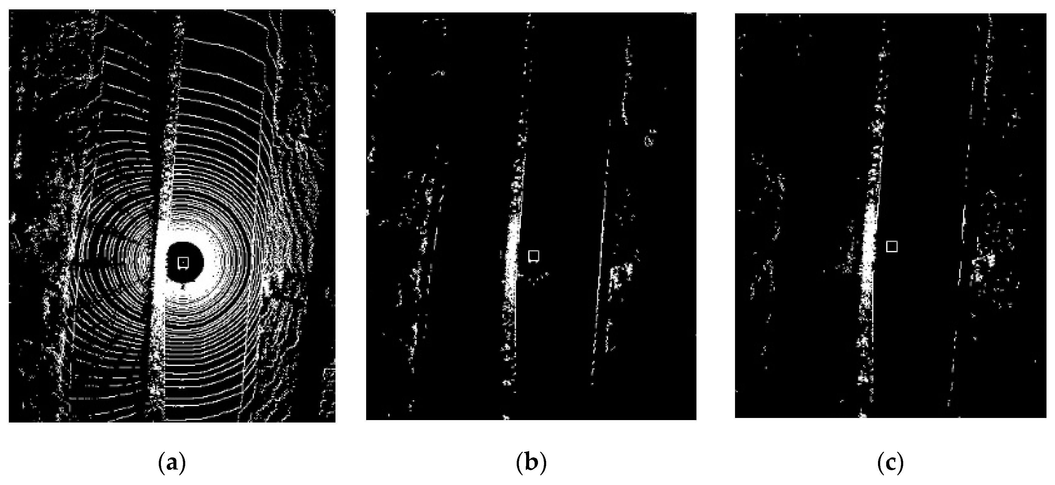
Figure 20.
Comparison between the ground segmentation method in [24] and the proposed method. (a) Real scene; (b) Original point cloud; (c) Result of method in [24]; (d) Result of the proposed method.


Figure 21.
Road curb detection result under different scenes. (a) An urban scene; (b) A snowy scene; (c) A field scene.
Figure 21.
Road curb detection result under different scenes. (a) An urban scene; (b) A snowy scene; (c) A field scene.

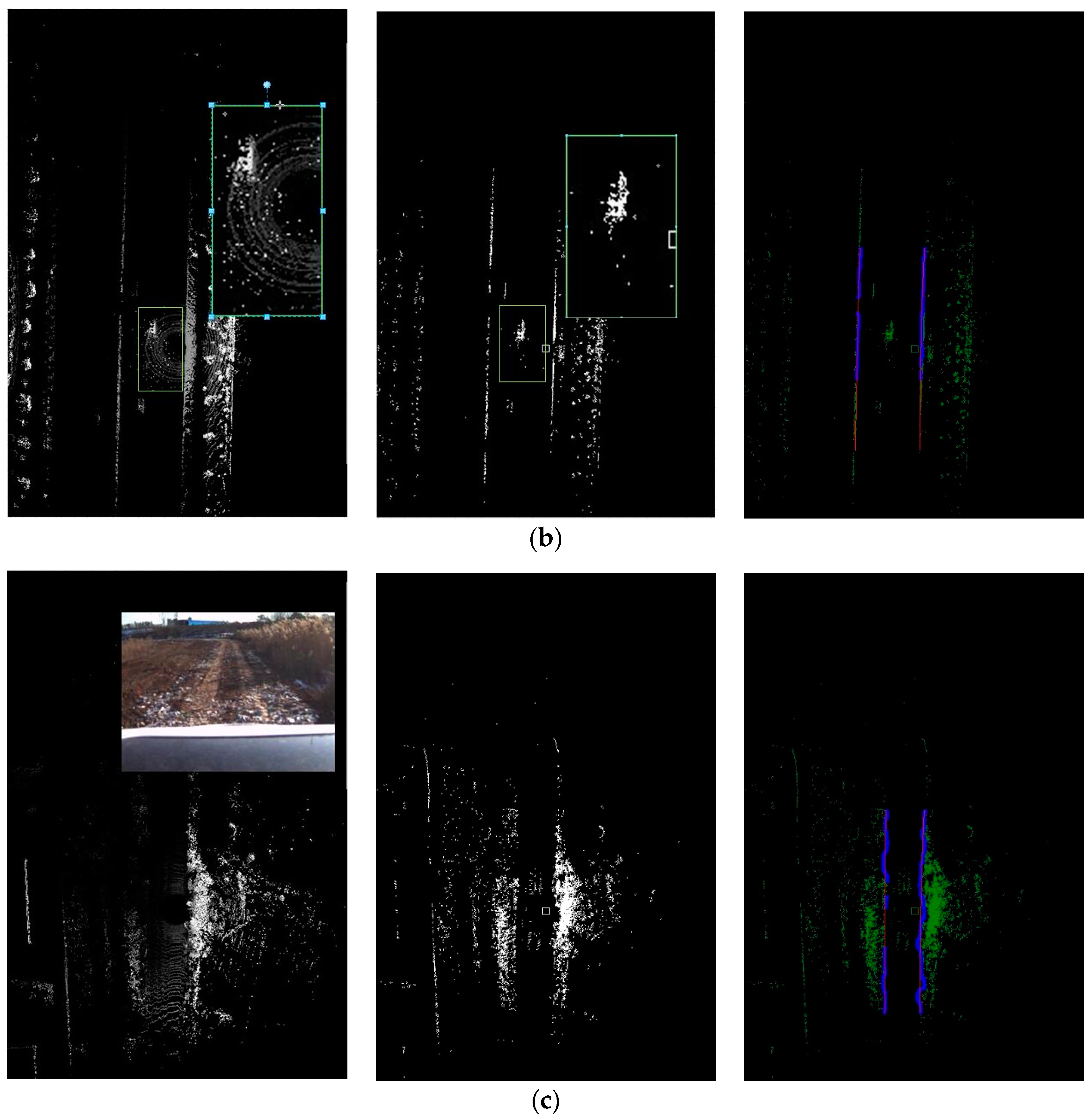
Figure 22.
Comparison between the road detection result of [24] and this work. (a) Raw point cloud; (b) Result of [24]; (c) Result of this work.

Figure 23.
The road curb detection time-consuming experiment.
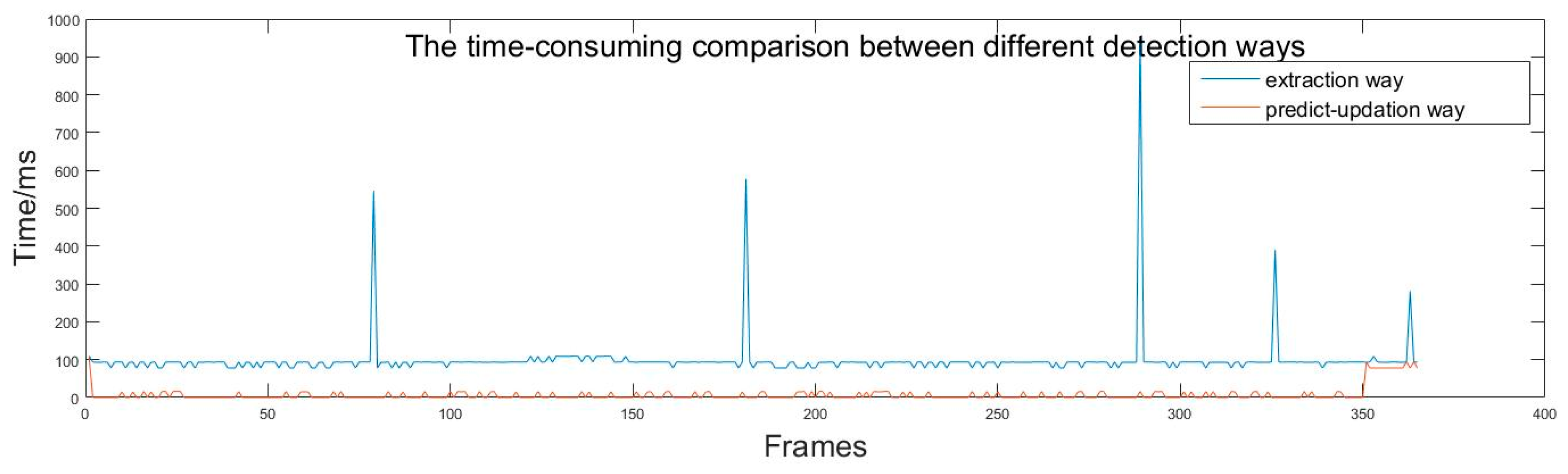
Figure 24.
Testing path.

Figure 25.
Result of curb detection in typical scenes. (a) Straight road; (b) Winding road.


Table 1.
The range and threshold for each feature.
| Feature | Beam Range (m) | Rotation Range | Threshold |
|---|---|---|---|
| MaxHD | [0, 45] | All | >3 cm |
| TangenAngle | All | [0, 300] || [600, 1200] || [1200, 1800] | >0.6 |
| RadiusRatio | [0, 50] | All | [0.9, 0.95] || [1.05, 1.1] |
| HDInRadius | All | All | >5 cm |
Table 2.
Threshold for each index.
| Index | Threshold |
|---|---|
| Road curb curvature | < 0.001 |
| Point number consisted the road curb | > 150 |
| Maximum difference of the y value between the detected points | > 200 |
| Variance of the width distribution | < 10 |
| Difference of the road width between two consecutive frames | < 10 |
Table 3.
Accuracy of the curb detection method.
| - | Scenes |
|---|---|
| Proposed method | Straight road |
| Winding road | |
| Method of [24] | Straight road |
| Winding road |
© 2017 by the authors. Licensee MDPI, Basel, Switzerland. This article is an open access article distributed under the terms and conditions of the Creative Commons Attribution (CC BY) license (http://creativecommons.org/licenses/by/4.0/).
Share and Cite
MDPI and ACS Style
Huang, R.; Chen, J.; Liu, J.; Liu, L.; Yu, B.; Wu, Y. A Practical Point Cloud Based Road Curb Detection Method for Autonomous Vehicle. Information 2017, 8, 93. https://doi.org/10.3390/info8030093
AMA Style
Huang R, Chen J, Liu J, Liu L, Yu B, Wu Y. A Practical Point Cloud Based Road Curb Detection Method for Autonomous Vehicle. Information. 2017; 8(3):93. https://doi.org/10.3390/info8030093
Chicago/Turabian StyleHuang, Rulin, Jiajia Chen, Jian Liu, Lu Liu, Biao Yu, and Yihua Wu. 2017. "A Practical Point Cloud Based Road Curb Detection Method for Autonomous Vehicle" Information 8, no. 3: 93. https://doi.org/10.3390/info8030093
Note that from the first issue of 2016, this journal uses article numbers instead of page numbers. See further details here.