Leak Location of Pipeline with Multibranch Based on a Cyber-Physical System


1
School of Automation, Northwestern Polytechnical University, Xi’an 710072, China
2
School of Information and Control Engineering, Liaoning Shihua University, Fushun 113001, China
3
CNPC Northeast Refining & Chemical Engineering Co. Ltd. Shenyang Company, Shenyang 110167, China
*
Author to whom correspondence should be addressed.
Information 2017, 8(4), 113; https://doi.org/10.3390/info8040113
Submission received: 28 August 2017
/
Revised: 12 September 2017
/
Accepted: 15 September 2017
/
Published: 22 September 2017
(This article belongs to the Special Issue Smart Sensing, Information Security and Control of Industrial Cyber-Physical Systems)
Abstract
:Data cannot be shared and leakage cannot be located simultaneously among multiple pipeline leak detection systems. Based on cyber-physical system (CPS) architecture, the method for locating leakage for pipelines with multibranch is proposed. The singular point of pressure signals at the ends of pipeline with multibranch is analyzed by wavelet packet analysis, so that the time feature samples could be established. Then, the Fischer-Burmeister function is introduced into the learning process of the twin support vector machine (TWSVM) in order to avoid the matrix inversion calculation, and the samples are input into the improved twin support vector machine (ITWSVM) to distinguish the pipeline leak location. The simulation results show that the proposed method is more effective than the back propagation (BP) neural networks, the radial basis function (RBF) neural networks, and the Lagrange twin support vector machine.
1. Introduction
Pipeline transportation is widely used in oil and gas transportation because of its safety, reliability and economy [1,2]. However, pipeline leakage can cause environment pollution and financial losses. Therefore it is important to detect and locate the leakage under pipeline working conditions [3].
Currently, most of the reports about leak detection systems based on data-driven techniques are directed at straight pipelines. According to data-driven methods, there are three main steps are necessary for leak detection and location based on signals analysis: feature extraction; feature selection, and; pattern recognition. Traditional feature extraction such as wavelet packet decomposition (WPD), empirical mode decomposition (EMD), and local mean decomposition (LMD) have been widely used in pipeline leak detection [4,5]. Moreover, the detection performance depends on the quality of the selected features, and the feature selection depends largely on prior knowledge [6]. Several research results have shown that pattern recognition such as support vector machine (SVM), least squares support vector machine (LSSVM), and least squares twin support vector machine (LSTSVM) have a powerful classification efficacy [7,8,9,10], and they are very suitable to effectively build the complex relationships in leak detection and location. Therefore, it is meaningful to establish twin support vector machine (TWSVM) for pipeline leak detection.
Pipelines with multibranch are quite common and leak detection for them is one of the most popular areas of research in this field [11]. Recently, some studies have shown that leakage from water-filled systems, such as the leakage of pipelines, can be well identified and localized by acoustic waves [12]. Acoustic leak detection methods have been studied, and their pipeline networks experiment has been presented [13,14]. Conventional leak detection system needs to connect instruments with the laying of cables. However, the geographical environment of pipeline laying, sometimes, is extremely bad and it is difficult to install cables. Furthermore, factors such as aging and material defects could affect the stability of signal transmission and increase maintenance costs. Therefore, the combination with wire transmission and wireless transmission [15] is adopted in long-distance pipeline leak detection systems.
If the leak detection system is used for branch pipeline is different from the one used for the main pipeline, data cannot communicate among different leak detection systems. When adding new sensors, the data structure of the main program needs to be amended and the extensibility is poor. In addition, lacking real-time data structure and algorithm, the information delay is quite common and larger errors could be produced in locating leakages. The network of cyber-physical system (CPS) is heterogeneous network [16], in other words, the network can contain different attributes simultaneously, and the information range and form of communication are unrestricted. In order to transfer the information between layers smoothly to meet the real-time requirement and to make it possible to detect and locate leaks of the pipeline with multibranch, the leakage location method based on CPS is proposed.
When utilizing CPS framework to detect the leakage of a pipeline with multibranch, first, the wavelet packet analysis is used to extract the time of singular point of the measured pressure signal, and then the time feature samples are input into the improved twin support vector machine (ITWSVM) to locate the leakage position.
The rest of this paper is organized as follows. Section 2 introduces the cyber-physical system design of pipelines with multibranch. The leak location method of pipelines with multibranch is proposed in Section 3. In Section 4, the simulation results for pipelines with multibranch are analyzed and discussed. Finally, Section 5 draws the main conclusions and puts forward the plan of future work.
2. Cyber-Physical Leak Location System Design
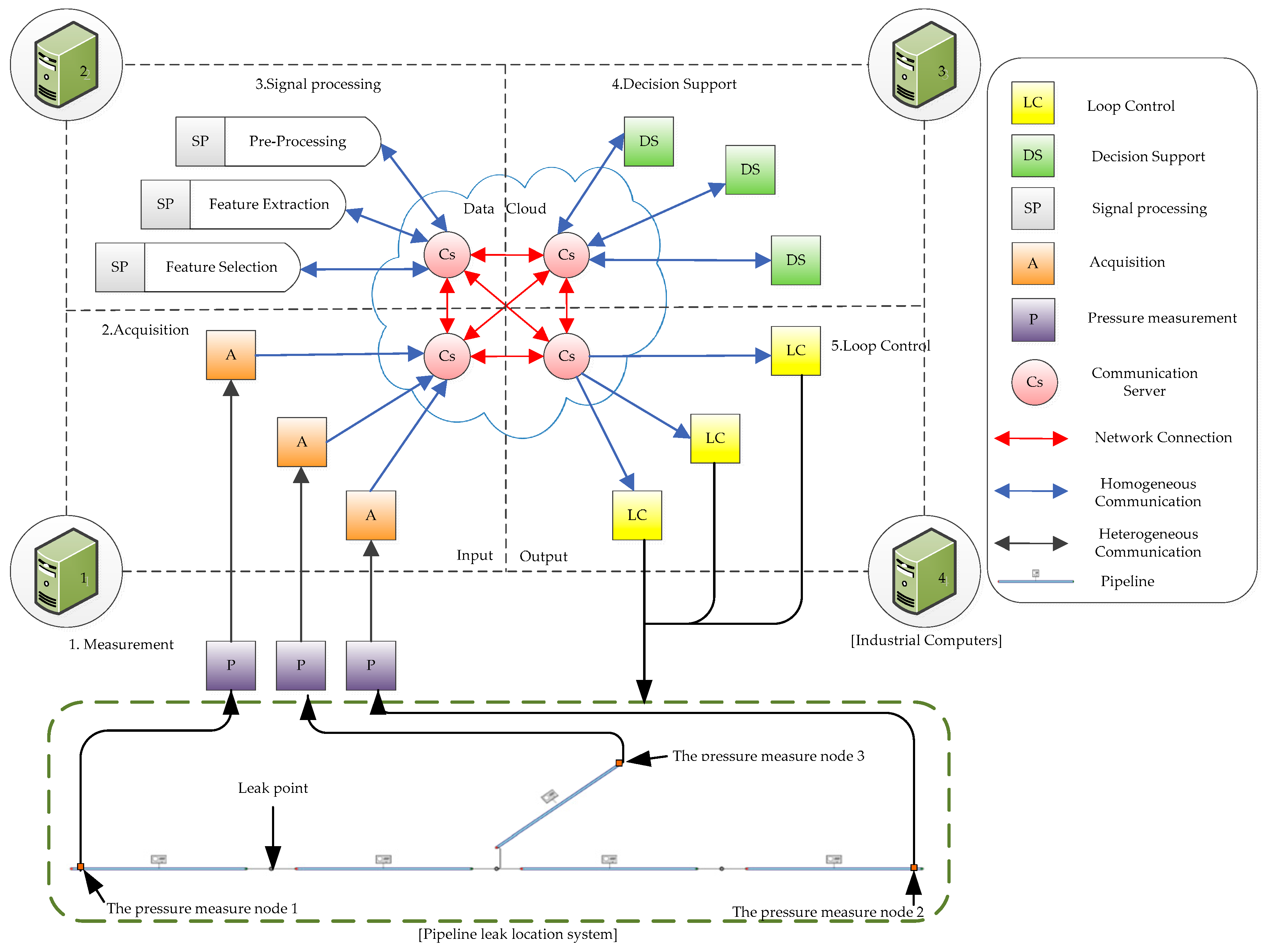
CPS is the integration of computation, communication, and a control loop, which improves the stability and reliability of physical applications [17]. In order to solve the problems about signal transmission between heterogeneous networks, the leak location method of the pipeline with multibranch is proposed in this paper. Based on CPS, a schematic of the pipeline leak location system is shown in Figure 1.
The measurement layer consists of a number of instruments, which can measure the values of internal pressure, flow and temperature of the pipeline. It can communicate with other units through the network.
The communication layer contains various networks according to actual conditions, such as Wi-Fi, Zigbee, and 3G/4G, as well as communication between the base station and the network node. Moreover, the communication between database and data processing unit server is included in this layer as well. Furthermore, the layer is responsible for data storing and transmitting.
The signal processing layer aims to reprocess the measured signals, to extract and to select features. Then feature vectors are input into the decision application layer through the communication layer.
The main purpose of the decision application is to remotely and visually monitor the work conditions of multibranch pipelines. If a leak occurs, it will sound an alarm and locate the position. Consequently, the decision application layer mainly consists of a decision monitoring unit and a decision processing unit. The decision monitoring unit includes the feature vectors from the signal processing layer. In the decision processing unit, the operators analyze and locate the leak position with using the measured data, which is provided by the decision monitoring unit.
The control layer executes the instructions, which are produced from the decision application layer and transmitted through the communication layer.
3. Leak Location Method of Pipeline with Multibranch
3.1. Wavelet Packet Analysis
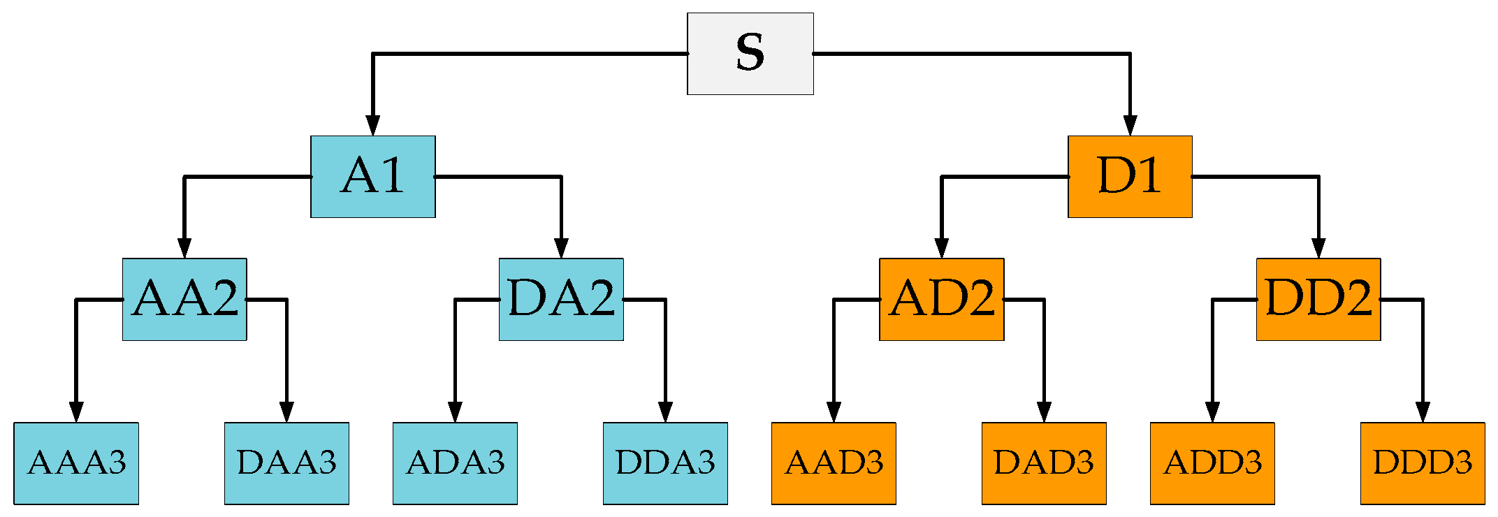
Wavelet packet analysis [18] is an effective time-frequency analysis technique for non-stationary signals. Multi-resolution analysis of wavelet packet transform decomposes signals into low frequency and high frequency. After that, the process continues to decompose the following layers until the preset level, thus the wavelet packet analysis has a better ability to make accurate local analysis. Moreover, wavelet packet analysis has better characteristics for furthering segmentation and refinement of the frequency band broadened with the increase of scale. Therefore, it is a precise analysis method with the characteristics of high frequency band width and low frequency band narrow. When the signal is decomposed by wavelet packets, a variety of wavelet basis functions can be adopted. For instance, the signal is decomposed by wavelet packets in three layer decomposition, as shown in Figure 2.
The signal is decomposed by wavelet packet decomposition tree and can be represented as
3.2. Improved Twin Support Vector Machine
Considering the binary classification problem, this paper assumes the training set is , , and makes matrix in represent the inputs of class , and matrix in represent the inputs of class . It aims to find a decision function as the objective function, so that the new data could be input into to get the output , which could be regarded as data categories.
Lagrangian twin support vector machine (LTSVM) constructs a pair of primal problems [19], one primal problem corresponding to one non-parallel plane. It aims to make the same class data samples have the nearest distance to the relevant plane and have adequate distances to the other plane.
The pair of nonparallel hyper-planes is illustrated as follows:
where , and , .
The pair of optimization problem for TWSVM can be formulated as
and
where and are parameters, and are the slack vectors, and is the proper dimension vector.
In order to get the solutions of optimization problems (3) and (4), this paper derives the dual problems as follows
and
where and are the Lagrangian multipliers, and , and is the proper dimension vector.
Let and , with satisfying the conditions of Karush-Kuhn-Tucker (KKT). Equations (5) and (6) are obtained as
The new point is assigned to class , which depends on Equations (7) and to which (8) is closer.
The decision function is shown as follows:
where is the absolute value.
Equations (5) and (6) can be represented as follows:
where is a positive definite matrix, when , Equation (10) is equal to Equation (5). Similarly, when , Equation (10) is equal to Equation (6).
There are many ways to deal with Equation (10). In this paper, the steepest descent algorithm is used to solve Equation (10). Equation (10) is transformed into an unconstrained optimization problem by using the complementary function [20].
Definition 1.
For arbitrary , mapping is a sort of complementary function, and such that
The Fischer-Burmeiste function is commonly used as a kind of complementary function and defined as :
are true.
Let , Equation (12) can be expressed as
As a consequence, Equation (13) equals to an unconstrained minimization problem:
The optimum solutions between complementary problem and the optimal problem are calculated by Equations (7) and (8).
Thus, the proposed algorithm is as follows:
Step 1: Initialization. Select initial point . Select parameters , , and set .
Step 2: Calculate the search direction: .
Step 3: If ( is the error requirement), the search will stop; otherwise, go to Step 4.
Step 4: Let become the smallest nonnegative integer which satisfies the inequality as follows: .
Step 5: Let ; go to step 2.
The theorem proves the proposed algorithm see Appendix A.
4. Simulation and Analysis
All the methods are implemented in MATLAB R2014a and Flowmaster V7 environments on a PC with an Intel Pentium processor (2.90 GHz) and 6 GB RAM.
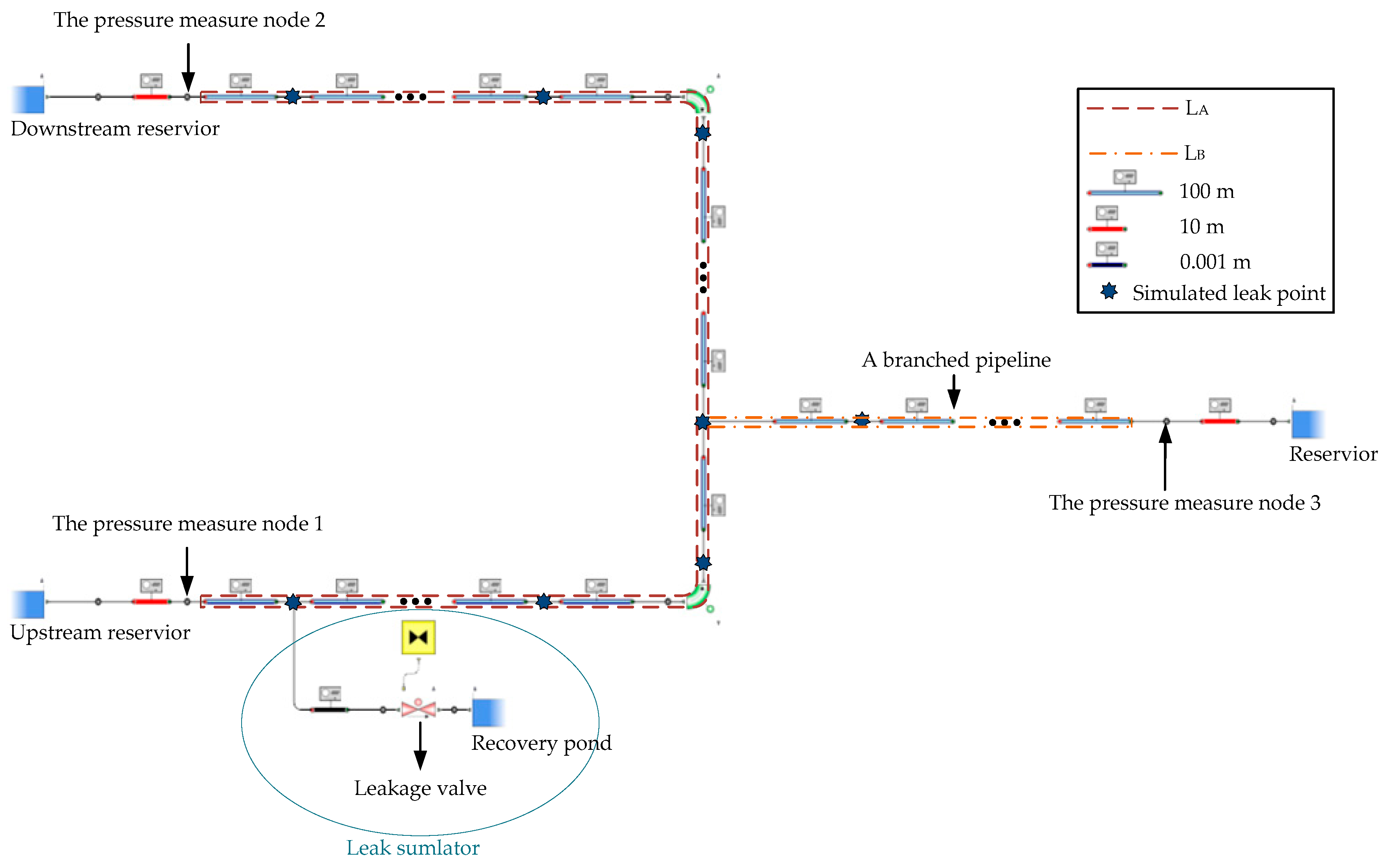
Leakage of the pipeline with the branch is simulated by Flowmaster software [21], and the establishment of the pipeline leak model is shown in Figure 3. According to the real pipeline environment, the elastic pipeline is applied to establish the pipeline leak model. The length of the main pipeline LA and the branch LB are 4000 m and 1000 m, respectively. The LA with outer diameter of 200 mm is used as the main pipeline, LB with outer diameter of 200 mm is connected to the larger one as the branch pipeline. The roughness of the inside pipeline wall is 0.025 mm. The oil reservoir height of constant head upstream, downstream and the branch are 300 m, 0 m and 0 m, respectively. The inlet volumetric flow rate is 0.1 m3/s. The pressure wave speed is 1000 m/s, and the external temperature is 20 degrees Celsius. To emulate leaks, flow ball valves are positioned at every 100 m from upstream, the leaking flow rate is 0.01 m3/s. Three pressure measure nodes are placed at node 1, node 2 and node 3. In addition, the pressure changes are calculated by the Flowmaster software. The sampling rate is 50 Hz, and the simulation time is 80 s. Next, the CPS is applied for locating leaks of the pipeline with the branch in a heterogeneous distribution environment.
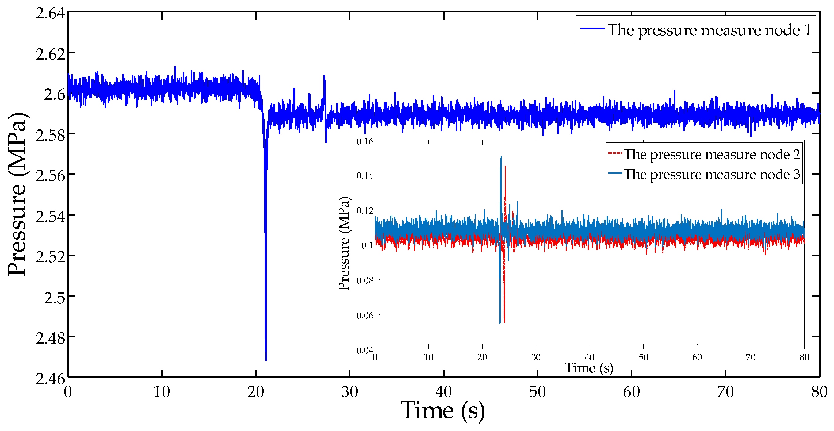
Because the Flowmaster software generates noiseless pressure signals, in order to simulate the real working conditions, the standard normal distribution random number is added to the pressure data collected at the boundary of the pipeline with the branch in the MATLAB experiment to approximate the actual conditions; thus, multiple simulation data is generated. There is a leakage at 20 s, whose aperture is 20 mm at 100 m from the pressure measure node 1. The waveform of the measured pressure is shown in Figure 4.
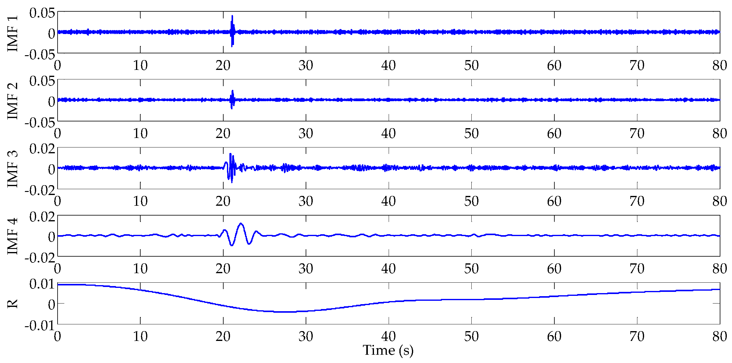
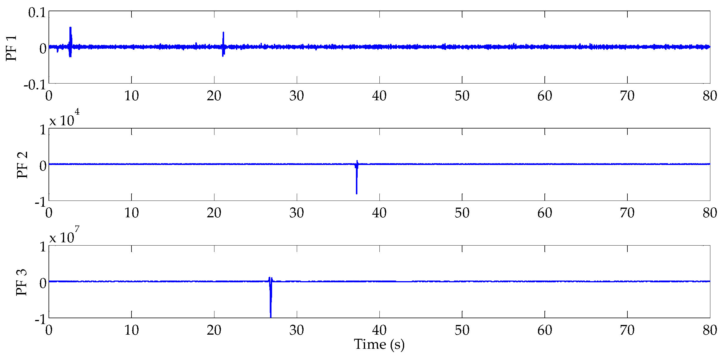
According to the measured pressure signal at the boundary of the pipeline with the branch, they are decomposed by the WPD of the best tree structure with Daubechies 3 (db3) in three layers. Using the best tree structure, the time of singular point of pressure signal is extracted. In order to verify the validity of signal singular points which are extracted by wavelet packet, we chose four intrinsic mode functions (IMFs) after decomposition derived from EMD, and we also acquired three production functions (PFs) after the decomposition derived from LMD. The results of signal decomposition with EMD and LMD are respectively shown in Figure 5, Figure 6 and Figure 7.
From Figure 5, Figure 6 and Figure 7, it can be shown that the wavelet packet analysis presents a powerful ability for extracting the signal singular point from measured pressure signals, compared with other methods like EMD and LMD. When the measured pressure signals are decomposed with EMD, due to the influence of the end effect, it is very difficult to accurately identify signal singular point. The LMD method is more relaxed than EMD in terms of decomposition conditions as the end effect is reduced and the over envelope phenomenon is avoided in the decomposition process. However, the end effect still affects the extraction for accurately signal singular point.
Thus, the wavelet packet analysis is used to extract pressure signal singular point at the boundary of the pipeline with the branch. The time of signal singular points of pressure of the 20-mm leakage aperture are collected at node 1, node 2, and node 3. Fifty cases are created, respectively. Sixty samples from each case are chosen for training the ITWSVM. Thus, 3000 samples of pressure singular point are selected. Moreover, 2500 samples are chosen as training samples and the others are using as testing samples. Partial samples are calculated and shown in Table 1.
In this simulation, three nodes (the time of signal singular point of pressure measure node 1, pressure measure node 2, and pressure measure node 3) are the inputs of the ITWSVM, and the output are different leakage locations. Therefore, different leakage locations can be identified according to the collected singular points of pressure signal via ITWSVM.
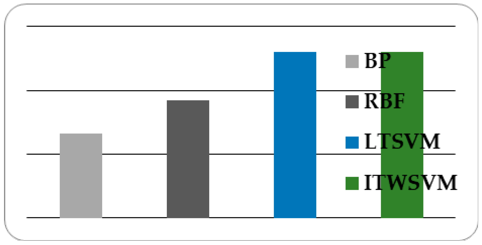
In order to compare leak location accuracy, the input and output for back propagation neural network (BP), radial basis function neural network (RBF), and LTSVM are the same as those for ITWSVM. This paper chooses a three-layer BP neural network whose middle layer node number is 15, using 200 iterations, and for which the learning rate is 0.01, and the minimum error is . In reference [19], the parameters are set to , and the parameter of LTSVM of is set to , error . It chooses ITWSVM of which parameters are also set to , and the steepest descent method parameters are set to and , error . This paper adopts the “One-versus-Rest” algorithm of multi-classification. Figure 8 shows the accuracy of four methods in leak localization.
From Figure 8, it can be seen that ITWSVM can achieve more accurate leak location, as the test accuracy (96.06%) is higher than the BP neural network (83.2%) and RBF neural network (88.4%). LTSVM and ITWSVM have the same objective function to achieve the same accuracy, but the computing time is different. The calculation time of four methods are separately shown in Table 2.
It can be seen in Table 2 that the ITWSVM improves the solution speed over that of LTSVM, because when solving the double objective function, the ITWSVM algorithm transforms the objective function with upper and lower bound constraints to unconstrained solution. Each iteration requires no matrix inversion computation, thus it reduces the amount of calculation and improves the solution speed.
5. Conclusions and Future Work
The leakage location of pipelines with multibranch under the framework of CPS can solve the problem about no sharing of data and no locating leaks simultaneously among multiple pipeline leak detection systems. Wavelet packet analysis is more suitable for extracting signal singular point of non-stationary pressure signals than EMD and LMD, and the computing time of ITWSVM is faster compared with other methods (BP, RBF and LTSVM). However, in real operation conditions, there is some external low frequency signal interference in pressure signals, which can cause location errors when using wavelet packet analysis. Future work will involve carrying out signal de-noising effectively and to extract true signal singular point. In addition, when the leakage aperture is smaller, the inflection point of the waveform is not easily distinguished. Thus, the small leaks will be studied in the future.
Acknowledgments
This work was supported by National Natural Science Foundation of China (61673199).
Author Contributions
Ping Li proposed the idea; Xianming Lang wrote this paper; Xianming Lang carried out the experiments and analyzed the data; Yan Li and Hong Ren analyzed the research data. All authors have read and approved the final manuscript.
Conflicts of Interest
The authors declare no conflict of interest.
Appendix A
The following theorem proves the proposed algorithm can insure the convergence.
Lemma A1.
If is not the solution of the complementary problems, the search direction is a descent direction at point , which satisfies the descent condition .
Proof of Lemma A1.
According to then . □
According to the definition of complementary function, because of , can be considered as a positive definite matrix, so the formula and are obtained. Therefore . Similarly, when , can be also proved.
Theorem A1.
If is the smallest non-negative integer that satisfies the inequality: , the solutions of this equation exist.
Proof of Theorem A1.
Assuming that this equation has no solution, for arbitrary positive integer , and that both sides of the inequality are divided by at the same time, letting , if there is no solution, , then . However, it is contradictory to the lemma, and therefore there is a , which makes true. □
Theorem A2.
Let be an infinite sequence generated by the algorithm, at least one point, and an arbitrary point be the solution of complementary problems (Equation (10)).
Proof of Theorem A2.
Because of , is the positive definite matrix. According to Theorem 5.4 in [22], it can be proved that the theorem is established. Similarly, when , it can be also proved. □
References
- Murvay, P.; Silea, I. A survey on gas leak detection and localization techniques. J. Loss Prev. Process Ind. 2012, 25, 966–973. [Google Scholar] [CrossRef]
- Datta, S.; Sarkar, S. A review on different pipeline fault detection methods. J. Loss Prev. Process Ind. 2016, 41, 97–106. [Google Scholar] [CrossRef]
- Verde, C.; Torres, L. Modeling and Monitoring of Pipelines and Networks: Advanced Tools for Automatic Monitoring and Supervision of Pipelines; Springer: Cham, Switzerland, 2017. [Google Scholar]
- Liang, W.; Zhang, L. A wave change analysis (WCA) method for pipeline leak detection using Gaussian mixture model. J. Loss Prev. Process Ind. 2012, 25, 60–69. [Google Scholar] [CrossRef]
- Liu, J.; Su, H.; Ma, Y.; Wang, G.; Wang, Y.; Zhang, K. Chaos characteristics and least squares support vector machines based online pipeline small leakages detection. Chaos Solitons Fractals 2016, 91, 656–669. [Google Scholar] [CrossRef]
- Sun, J.; Xiao, Q.; Wen, J.; Wang, F. Natural gas pipeline small leakage feature extraction and recognition based on LMD envelope spectrum entropy and SVM. Measurement 2014, 55, 434–443. [Google Scholar] [CrossRef]
- Mandal, S.K.; Chan, F.T.S.; Tiwari, M.K. Leak detection of pipeline: An integrated approach of rough set theory and artificial bee colony trained SVM. Expert Syst. Appl. 2012, 39, 3071–3080. [Google Scholar] [CrossRef]
- Qu, Z.; Feng, H.; Zeng, Z.; Zhuge, J.; Jin, S. A SVM-based pipeline leakage detection and pre-warning system. Measurement 2010, 43, 513–519. [Google Scholar] [CrossRef]
- Ni, L.; Jiang, J.; Pan, Y. Leak location of pipelines based on transient model and PSO-SVM. J. Loss Prev. Process Ind. 2013, 26, 1085–1093. [Google Scholar] [CrossRef]
- Lang, X.; Li, P.; Hu, Z.; Ren, H.; Li, Y. Leak detection and location of pipelines based on LMD and least squares twin support vector machine. IEEE Access 2017, 5, 8659–8668. [Google Scholar] [CrossRef]
- Verde, C.; Torres, L.; González, O. Decentralized scheme for leaks’ location in a branched pipeline. J. Loss Prev. Process Ind. 2016, 43, 18–28. [Google Scholar] [CrossRef]
- Martini, A.; Troncossi, M.; Rivola, A. Leak detection in water-filled small-diameter polyethylene pipes by means of acoustic emission measurements. Appl. Sci. 2017, 7, 2. [Google Scholar] [CrossRef]
- Martini, A.; Troncossi, M.; Rivola, A. Automatic leak detection in buried plastic pipes of water supply networks by means of vibration measurements. Shock Vib. 2015, 2015, 165304. [Google Scholar] [CrossRef]
- Yazdekhasti, S.; Piratla, K.R.; Atamturktur, S.; Khan, A. Experimental evaluation of a vibration-based leak detection technique for water pipelines. Struct. Infranstruct. Eng. 2017. [Google Scholar] [CrossRef]
- Junie, P.; Dinu, O.; Eremia, C.; Stefanoiu, D.; Petrescu, C.; Savulescu, I. A WSN based monitoring system for oil and gas transportation through pipelines. IFAC Proc. Vol. 2012, 45, 1796–1801. [Google Scholar] [CrossRef]
- Yuan, X.; Anumba, C.J.; Parfitt, M.K. Cyber-physical systems for temporary structure monitoring. Autom. Constr. 2016, 66, 1–14. [Google Scholar] [CrossRef]
- Morgan, J.; O’Donnell, G.E. Cyber-physical process monitoring systems. J. Intell. Manuf. 2015. [Google Scholar] [CrossRef]
- Lei, D.; Yang, L.; Xu, W.; Zhang, P.; Huang, Z. Experimental study on alarming of concrete micro-crack initiation based on wavelet packet analysis. Constr. Build. Mater. 2017, 149, 716–723. [Google Scholar] [CrossRef]
- Shao, Y.; Chen, W.; Zhang, J.; Wang, Z.; Deng, N. An efficient weighted Lagrangian twin support vector machine for imbalanced data classification. Pattern Recogn. 2014, 47, 3158–3167. [Google Scholar] [CrossRef]
- Zhang, X. Study on the Algorithms for some Optimization Problems and Applications. Ph.D. Thesis, Xidian University, Xi’an, China, 2011. [Google Scholar]
- Jeong, U.; Kim, Y.H.; Kim, J.; Kim, T.; Kim, S.J. Experimental evaluation of permanent magnet probe flowmeter measuring high temperature liquid sodium flow in the ITSL. Nucl. Eng. Des. 2013, 265, 566–575. [Google Scholar] [CrossRef]
- Chen, J.; Pan, S. A descent method for a reformulation of the second-order cone complementarity problem. J. Comput. Appl. Math. 2008, 213, 547–558. [Google Scholar] [CrossRef]
Figure 1.
Schematic of pipeline leak location system based on cyber-physical system.

Figure 2.
Wavelet packet decomposition of the signal S.

Figure 3.
Leak model of the pipeline with the branch realized in Flowmaster.

Figure 4.
Pressure original signal of 20-mm leakage aperture at 100 m from the measure node 1.

Figure 5.
Wavelet packet decomposition (WPD) for pipeline inlet pressure signal of 20-mm leakage aperture.
Figure 5.
Wavelet packet decomposition (WPD) for pipeline inlet pressure signal of 20-mm leakage aperture.
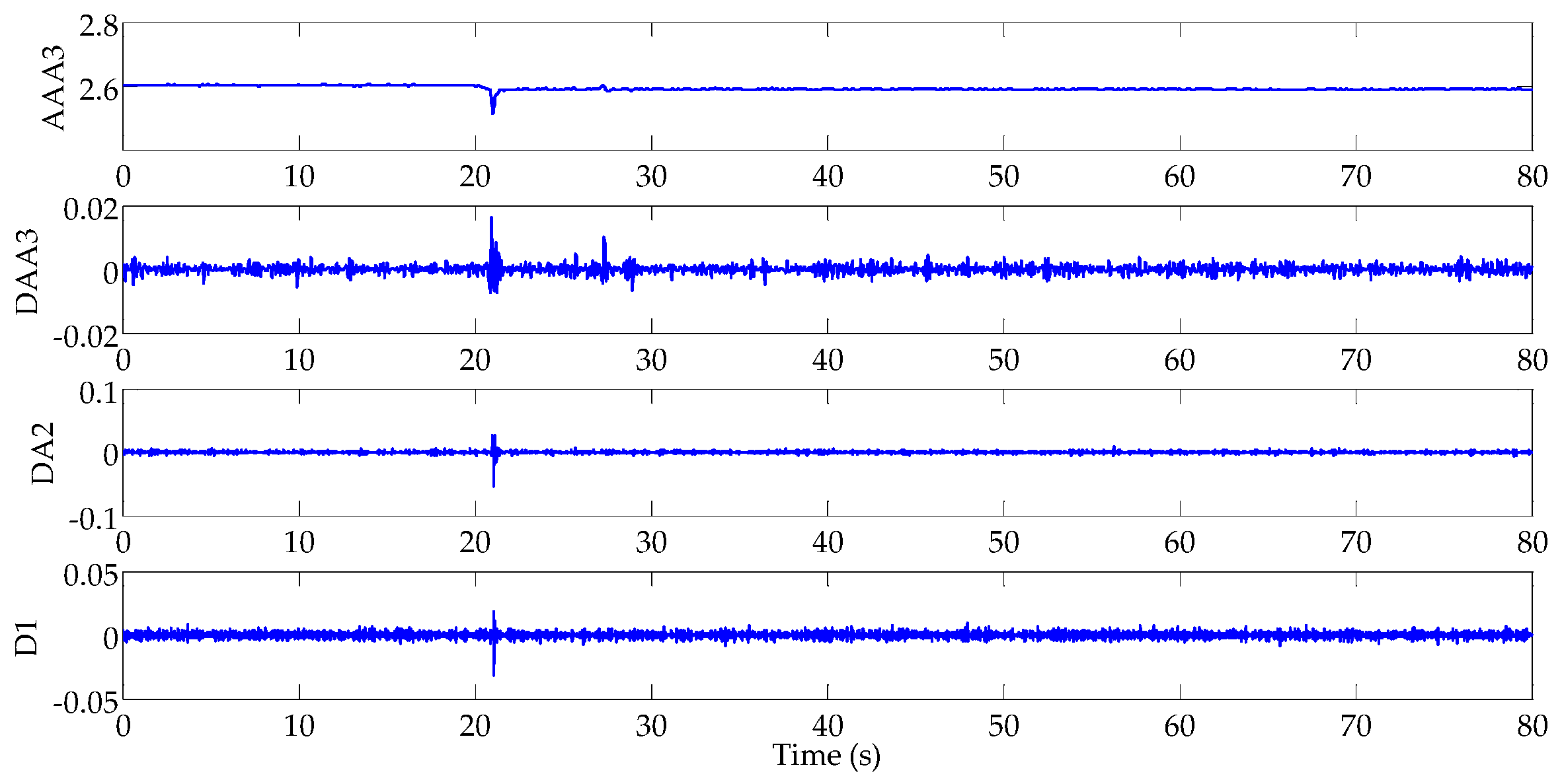
Figure 6.
Empirical mode decomposition (EMD) for pipeline inlet pressure signal of 20-mm leakage aperture.
Figure 6.
Empirical mode decomposition (EMD) for pipeline inlet pressure signal of 20-mm leakage aperture.

Figure 7.
Local mean decomposition (LMD) for pipeline inlet pressure signal of 20-mm leakage aperture.
Figure 7.
Local mean decomposition (LMD) for pipeline inlet pressure signal of 20-mm leakage aperture.

Figure 8.
Accuracy comparison of four methods in leakage localization.

Table 1.
Partial data for the ends of pipeline with the branch under pressure singular value.
| Leakage Position | Signal Singular Point of Pressure Measure Node 1 (s) | Signal Singular Point of Pressure Measure Node 2 (s) | Signal Singular Point of Pressure Measure Node 3 (s) |
|---|---|---|---|
| 100 m from upstream | 21.06 | 24.1 | 23.3 |
| 500 m from upstream | 21.38 | 23.78 | 22.98 |
| 1000 m from upstream | 21.78 | 23.38 | 22.58 |
| 1500 m from upstream | 22.18 | 22.98 | 22.18 |
| 2000 m from upstream | 22.58 | 22.58 | 21.78 |
| 2500 m from upstream | 22.98 | 22.18 | 22.18 |
| 3000 m from upstream | 23.38 | 21.78 | 22.58 |
| 3500 m from upstream | 23.78 | 21.38 | 22.98 |
| 4000 m from upstream | 24.06 | 20.98 | 23.42 |
| 500 m from branch junction | 22.98 | 22.98 | 21.38 |
| 1000 m from branch junction | 23.62 | 23.42 | 20.98 |
Table 2.
Computation time comparison of four methods for leakage location. Back propagation neural network (BP); radial basis function neural network (RBF); Lagrangian twin support vector machine (LTSVM).
Table 2.
Computation time comparison of four methods for leakage location. Back propagation neural network (BP); radial basis function neural network (RBF); Lagrangian twin support vector machine (LTSVM).
| Method | Computation (s) | Accuracy (%) |
|---|---|---|
| BP | 5.43 | 83.2 |
| RBF | 1.82 | 88.4 |
| LTSVM | 5.262 | 96.06 |
| The proposed method | 0.267 | 96.06 |
© 2017 by the authors. Licensee MDPI, Basel, Switzerland. This article is an open access article distributed under the terms and conditions of the Creative Commons Attribution (CC BY) license (http://creativecommons.org/licenses/by/4.0/).
Share and Cite
MDPI and ACS Style
Lang, X.; Li, P.; Li, Y.; Ren, H. Leak Location of Pipeline with Multibranch Based on a Cyber-Physical System. Information 2017, 8, 113. https://doi.org/10.3390/info8040113
AMA Style
Lang X, Li P, Li Y, Ren H. Leak Location of Pipeline with Multibranch Based on a Cyber-Physical System. Information. 2017; 8(4):113. https://doi.org/10.3390/info8040113
Chicago/Turabian StyleLang, Xianming, Ping Li, Yan Li, and Hong Ren. 2017. "Leak Location of Pipeline with Multibranch Based on a Cyber-Physical System" Information 8, no. 4: 113. https://doi.org/10.3390/info8040113
Note that from the first issue of 2016, this journal uses article numbers instead of page numbers. See further details here.