
A Novel Hybrid BND-FOA-LSSVM Model for Electricity Price Forecasting

School of Economics and Management, North China Electric Power University, Beijing 102206, China
*
Author to whom correspondence should be addressed.
Information 2017, 8(4), 120; https://doi.org/10.3390/info8040120
Submission received: 31 August 2017
/
Revised: 21 September 2017
/
Accepted: 25 September 2017
/
Published: 28 September 2017
(This article belongs to the Section Artificial Intelligence)
Abstract
:Accurate electricity price forecasting plays an important role in the profits of electricity market participants and the healthy development of electricity market. However, the electricity price time series hold the characteristics of volatility and randomness, which make it quite hard to forecast electricity price accurately. In this paper, a novel hybrid model for electricity price forecasting was proposed combining Beveridge-Nelson decomposition (BND) method, fruit fly optimization algorithm (FOA), and least square support vector machine (LSSVM) model, namely BND-FOA-LSSVM model. Firstly, the original electricity price time series were decomposed into deterministic term, periodic term, and stochastic term by using BND model. Then, these three decomposed terms were forecasted by employing LSSVM model, respectively. Meanwhile, to improve the forecasting performance, a new swarm intelligence optimization algorithm FOA was used to automatically determine the optimal parameters of LSSVM model for deterministic term forecasting, periodic term forecasting, and stochastic term forecasting. Finally, the forecasting result of electricity price can be obtained by multiplying the forecasting values of these three terms. The results show the mean absolute percentage error (MAPE), root mean square error (RMSE) and mean absolute error (MAE) of the proposed BND-FOA-LSSVM model are respectively 3.48%, 11.18 Yuan/MWh and 9.95 Yuan/MWh, which are much smaller than that of LSSVM, BND-LSSVM, FOA-LSSVM, auto-regressive integrated moving average (ARIMA), and empirical mode decomposition (EMD)-FOA-LSSVM models. The proposed BND-FOA-LSSVM model is effective and practical for electricity price forecasting, which can improve the electricity price forecasting accuracy.
1. Introduction
With the constant advance of electricity market reform, electricity price forecasting has become an important and valuable tool [1]. In the day-ahead electricity market, the electric energy trade and settlement are performed based on the market clearing price (MCP), which directly impacts the earnings of market participants. For independent power producers, they should submit the bidding curves according to accurately forecasted electricity price, which can reduce the market risk and maximize their profits. For power supply enterprises, they need optimally allocate the purchasing electricity in spot market and bilateral contract market according to accurately forecasted electricity price. For electricity supervision departments, they also use the forecasted electricity price information to supervise the electricity market, which can guarantee the healthy and sustainable development of electricity market. Therefore, accurate electricity price forecasting is quite important, which has become common concerns of electricity market participants [2].
Generally speaking, the electricity price will be influenced by several factors, such as power load demand, transmission congestion, economic development, and generator available capacity [3]. The electricity price time series hold the characteristics of volatility and randomness, which make accurate electricity price forecasting hard work [4,5]. In the past years, many researchers have made extensive efforts to develop the electricity price forecasting models and algorithms. There are mainly two kinds of forecasting methods for electricity price, which are conventional time-series statistical method and the emerging artificial intelligent method. For the conventional time-series statistical method, it holds the assumption that the electricity price has linear relationship with its influencing factors. This kind of forecasting technique mainly includes the auto-regressive integrated moving average (ARIMA) [6,7,8] method and generalized autoregressive conditional heteroscedasticity (GARCH) [9,10,11]. However, in fact, the relationships between electricity price and its influencing factors are not linear. So, the electricity price forecasting performance is unsatisfactory, and the forecasting accuracy needs to be improved for this kind of forecasting method. Under this background, a new electricity price forecasting technique, namely, the artificial intelligent method, was developed. For artificial intelligent-based electricity price forecasting method, there is no longer the assumption of linear relationships between electricity price and its influencing factors, which can effectively cover the shortages of conventional time-series statistical method. This kind of forecasting technique mainly includes artificial neural networks [12,13], fuzzy neural networks [14], extreme learning machines [15,16], and support vector machines [17,18]. However, there is also weakness for artificial intelligent forecasting method, namely the model parameters need to be set first, such as the kernel parameters of support vector machines and neuron number of neural networks. This is really difficult for electricity price forecasting handlers. To solve this issue, an intelligent optimization algorithm is usually used to automatically determine the parameters of artificial intelligent forecasting models, such as particle swam optimization (PSO) [19,20] and genetic algorithm (GA) [21,22].
Least square support vector machine (LSSVM) is a kind of improved algorithm of support vector machine, which has been used for many forecasting problems such as wind speed prediction [23], carbon price forecasting [24], electricity consumption forecasting [25,26], and network traffic forecasting [27]. However, it has rarely employed to forecast electricity price. Therefore, this paper will use the LSSVM model to forecast electricity price. Meanwhile, to improve the forecasting performance, a new intelligent optimization algorithm, namely, fruit fly optimization algorithm (FOA), is used to automatically determine the parameters of LSSVM model because the FOA shows superiorities over other intelligent optimization algorithms, which include short program code, quick convergence and high identification accuracy [28,29]. Considering the nonlinear and nonstationary characteristics of electricity price time series, the Beveridge-Nelson decomposition (BND) method is also used to decompose electricity price time series in this paper, which aims to improve the forecasting accuracy of electricity price. Therefore, this paper proposes a new electricity price forecasting method, namely, BND-FOA-LSSVM. To verify the applicability and effectiveness of this proposed BND-FOA-LSSVM electricity price forecasting method, a case study is selected, and its forecasting result is compared with other methods.
The remaining part of the paper is organized as follows. Section 2 introduces the basic theories of BND, FOA and LSSVM. Section 3 elaborates the proposed BND-FOA-LSSVM electricity price forecasting model. A case study is performed in Section 4, and the discussions related to forecasting performances of different methods are given in Section 5. Section 6 draws the conclusions.
2. Basic Theories of BND, FOA, and LSSVM
2.1. BND Method
For decomposing the non-stationary time series, two researchers, Stephen Beveridge and Charles Nelson, put forward the Beveridge-Nelson decomposition (BND) method in 1981 [30]. The data series with the first order co-integration characteristic can be decomposed into permanent term and transitory trend. The permanent term includes deterministic trend and stochastic trend, and the transitory trend has a stationary process with a zero average value, which can be named as the periodic term [31,32].
When the BND method is used to decompose time series, it is essential to identify whether the time series satisfies first order stationary or not. If satisfied, the detailed procedures of BND method for electricity price time series are as below.
Set the natural logarithm of electricity price time series as lnP. According to the Wold theorem, it can have:
where , Pt is the electricity price at time t, μ is the mean value of in the long run, εt ~ , t is the time period, and λi is the coefficient.
The expected value of Equation (1) is:
where E is the computation process of expected value for each variable.
Based on the BND theorem, the deterministic term DTt of electricity price time series can be decomposed as:
where DTt represents the deterministic term at time t, and lnP0 is the initial value of natural logarithm value of electricity price.
Morley pointed out that the time series can be much more accurately forecasted through employing a stationary univariate AR (Auto Regressive) [33], namely:
where .
Under the normality assumption, the minimum mean squared error (MMSE) of j-period ahead forecast of the first difference of ΔlnPt is:
Tt, the total trend term of time series, is identified as the MMSE prediction of the long-term level of the series. It is equivalent to the present level of the series plus the infinite sum of the MMSE of j-period ahead first difference forecasts, namely:
where Tt is the total trend term of time series.
Then, the total trend term of lnPt can be obtained, namely:
Meanwhile, the periodic term of lnPt can be expressed as:
where Ct is the periodic term at time t.
The random impulse term can be computed as:
where RTt demonstrates the random term at time t.
2.2. FOA
Inspired by the food-finding behavior of the fruit fly, a new swarm intelligence optimization algorithm was proposed by researcher Pan in 2012, namely the fruit fly optimization algorithm (FOA) [34]. Currently, the FOA has been employed in many practical issues, such as power load forecasting [35], oil and gold prices forecasting [36], and ship motion prediction [37]. In this paper, the FOA is used for parameters determination of the LSSVM model for electricity price forecasting.
The FOA includes the following four steps.
Step 1: Parameters setting.
The primary parameters of FOA comprise the initial fruit fly swarm location (X_axis, Y_axis), the number of fruit flies SearchAgents_no; the maximum number of iterations Max_iteration; and the random flight distance range FR.
Step 2: Population initialization.
As a swarm based algorithm, the initial population (Xi, Yi) of fruit flies in FOA can be given according to the random flight direction and the distance for food finding of an individual fruit fly by using osphresis.
Xi = X_axis + Random Value
Yi = Y_axis + Random Value
Step 3: Population evaluation.
In this step, the distance of food location to the origin (Dist) is firstly calculated, and then the smell concentration judgment value (S) can be calculated as follows:
By substituting Si into the smell concentration judgment function (also called Fitness function), the smell concentration (Smelli) of fruit fly location can be obtained, namely
Finally, the optimal fruit fly can be found which has the optimized smell concentration among all the fruit flies, and the fitness function value can also be determined, namely
Step 4: Selection operation.
After the optimal food location with the optimized smell concentration value is found, all fruit flies will fly toward it by using their visions. Then, the positions and smell concentration values of fruit flies will be updated. Repeat steps 2 and 3 and perform the iterative optimization until the terminal criterion is satisfied. Then, the optimal location and smell concentration values can be determined.
Smellbest = bestSmell
2.3. LSSVM Model
The least square support vector machine (LSSVM) model is a kind of emerging artificial intelligent technique, which can be used for forecasting issues and classification issues [38]. Compared with the support vector machine, the LSSVM alleviates convex quadratic programming based on structural risk minimization with a regularization constraint set on model weight [39]. The LSSVM has the advantages of setting slackness by an equality constraint and solving the regression problem as a set of linear equations, which can provide faster training and higher accuracy compared with support vector machine (SVM). The basic theory of LSSVM model is illustrated as below.
Set a series of samples , regarding as the input vector and as the corresponding output value of sample i. By using a nonlinear function φ, the electricity price data are mapped to a higher dimensional space from the original feature space, namely:
where w is the weight vector, and b is the error.
f(x) = wTϕ(x) + b
In the original space, the LSSVM formula with an equality constraint can be represented as
where C is regularization parameter, and ξi is slackness variable.
Then, the Lagrangian function L can be obtained as:
where ai is Lagrange multiplier.
The conditions of Karush-Kuhn-Tucker (KKT) for optimality are determined by
Removing the variables w and ξi, the optimization process can be transformed into the linear equation as below:
where Q = [1,…,1]T, A = [a1,a2,…,am]T; Y = [y1,y2,…,ym]T. In line with the Mercer’s condition, the Kernel function can be expressed as:
K(xi,xj) = ϕ(xi)Tϕ(xj)
Then, the LSSVM model for regression can be written as:
Since the radial basis function (RBF) has a fewer parameters to be set and a superior overall performance, it is selected to be the Mercer kernel function K(x,xi) in this paper, which is shown in Equation (26).
Therefore, there are two parameters which are needed to be determined for LSSVM model, which are the regularization parameter “C” and RBF kernel width “σ”. In this paper, these two parameters of LSSVM model will be optimally determined by a new intelligent optimization algorithm FOA for electricity price forecasting.
3. The Proposed Novel Hybrid BND-FOA-LSSVM Model for Electricity Price Forecasting
In this paper, a novel hybrid BND-FOA-LSSVM model is proposed for electricity price forecasting, which aims to improve the forecasting accuracy of electricity price. Since electricity price time series hold the characteristics of volatility and randomness, the BND method is firstly employed to decompose the initial electricity price time series into deterministic term, periodic term, and stochastic term. Then, the LSSVM model will be utilized to respectively forecast these three decomposed terms, and the parameters of LSSVM model will be optimized and determined by using FOA. Finally, the forecasted electricity price can be obtained by multiplying the forecasting results of three decomposed terms.
The detailed procedures of the proposed hybrid BND-FOA-LSSVM model for electricity price forecasting are elaborated as follows.
Step 1: Unit root test.
When the BND method is used, it is required to examine whether the logarithmic sequences of initial electricity price time series are first order stationary. The Augmented Dickey-Fuller (ADF) method is employed to conduct unit root test. If it satisfies the stationary condition, we can proceed to the next step.
Step 2: Initial electricity price time series decomposition.
After the first order stationary of logarithmic sequence of initial electricity price time series is confirmed, the initial electricity price time series can be decomposed into deterministic term, periodic term, and stochastic term.
Step 3: Parameters’ setting.
In FOA, four parameters are needed to be initialized, which are the initial fruit fly swarm location (X_axis, Y_axis); the number of fruit flies SearchAgents_no; the maximum number of iterations Max_iteration; and the random flight distance range FR. In this paper, we set (X_axis, Y_axis) ⊂ [0, 1], SearchAgents_no = 20, Max_iteration = 100, and FR ⊂ [−10, 10].
Step 4: Optimization starts.
The fitness function needs to be firstly determined through employing FOA to determinate the optimal two parameters values of LSSVM model. In this study, the root mean square error (RMSE) shown in Equation (27) is used to build the fitness function.
where x(k) is actual value of electricity price at time k; is forecasting value of electricity price at time k.
The FOA starts to optimize two parameters of LSSVM model by creating a series of random solutions. The smell concentration judgment value Si of fruit fly i is employed to represent two parameters of LSSVM model. The optimal smell concentration judgment value of fruit fly will be updated at each iteration, and the corresponding optimal parameters of LSSVM model in current stage can be obtained. Assumed that the actual electricity price data series is used in the first iteration, and then the forecasting (fitting) electricity price series can be calculated based on the built LSSVM model. Then, the fitness function can be confirmed by minimizing the RMSE of forecasting electricity price data points, namely
Step 5: Optimization ends.
Through the whole iteration process, different values of RMSEs will be generated, and the minimum RMSE will be found when the optimization process comes to the end. When the max iterative number is reached, the optimization process ends. Then, the optimal values of parameters “σ” and “c” can be obtained, and the LSSVM model optimized by FOA can be established. Finally, the future electricity price can be forecasted.
The procedure of the proposed BND-FOA-LSSVM model for electricity price forecasting is depicted in Figure 1.
4. Case Study
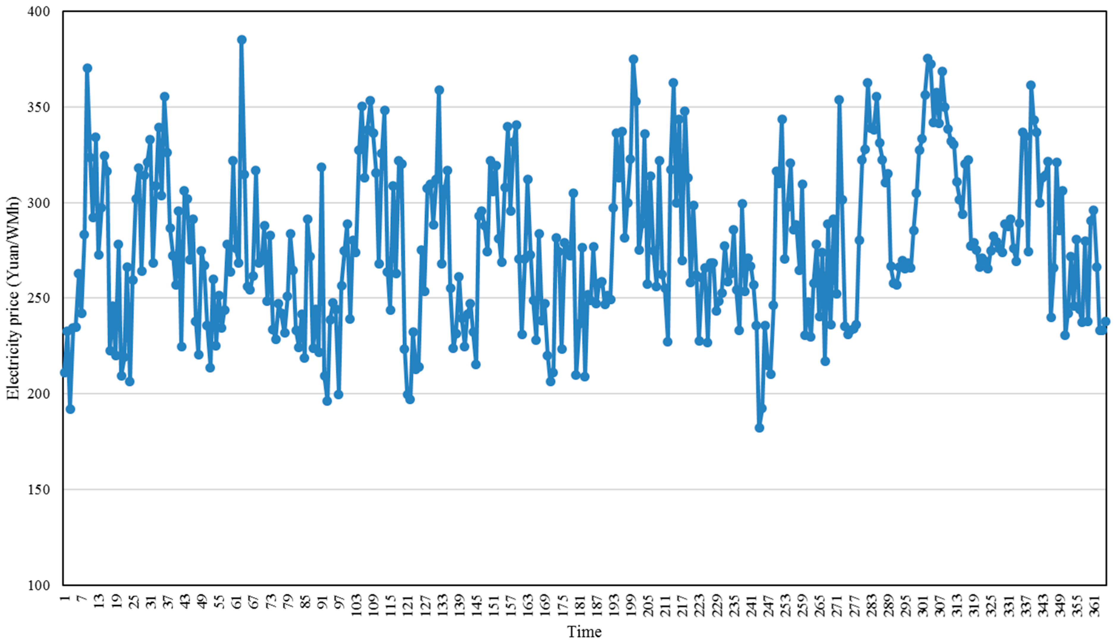
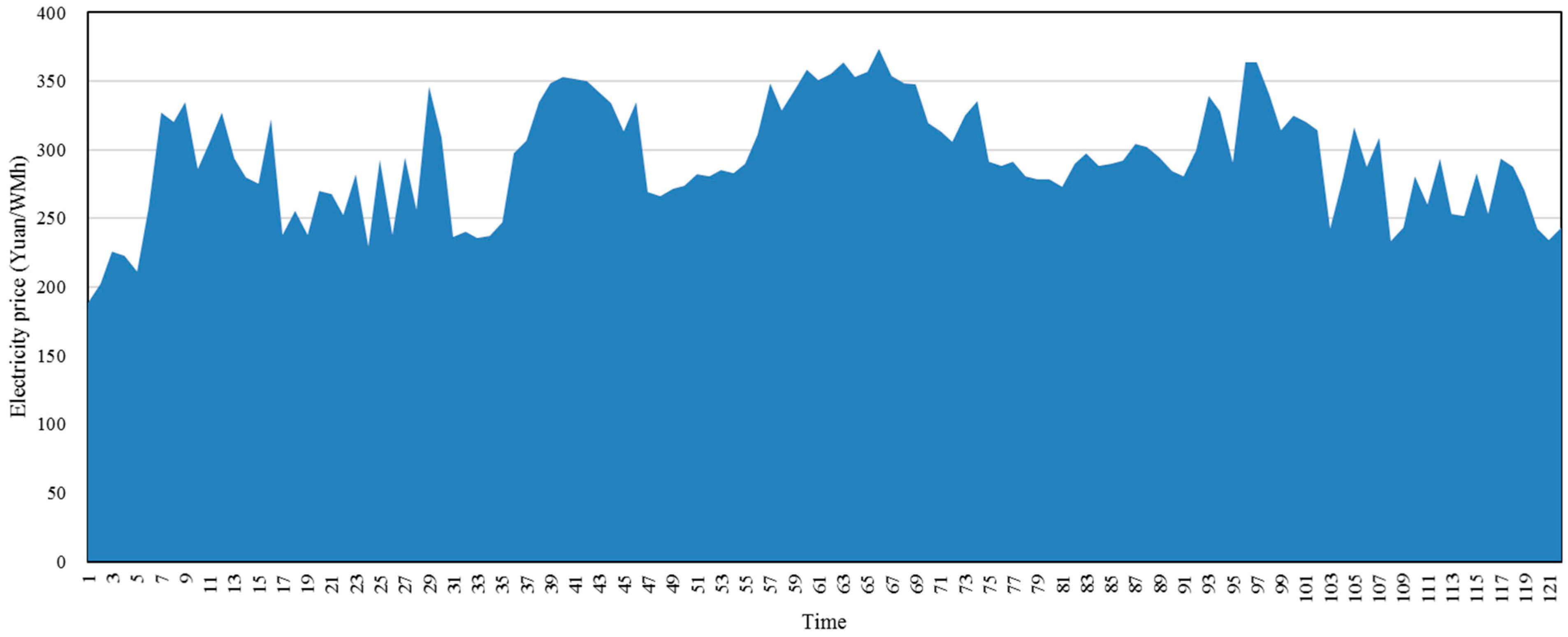
In this paper, the daily electricity price in the northeast power grid of China is used to perform case study and validate the forecasting performance of the proposed hybrid BND-FOA-LSSVM model for electricity price forecasting. The sample set contains one year (365 days) of daily electricity price data points ranging from 1 January to 31 December, which are shown in Figure 2. Of these, 243 daily electricity price data points from 1 January to 31 August are treated as training sample set, and the remaining 122 electricity price data points from 1 September to 31 December are considered as a testing sample set.
4.1. Electricity Price Decomposition Result
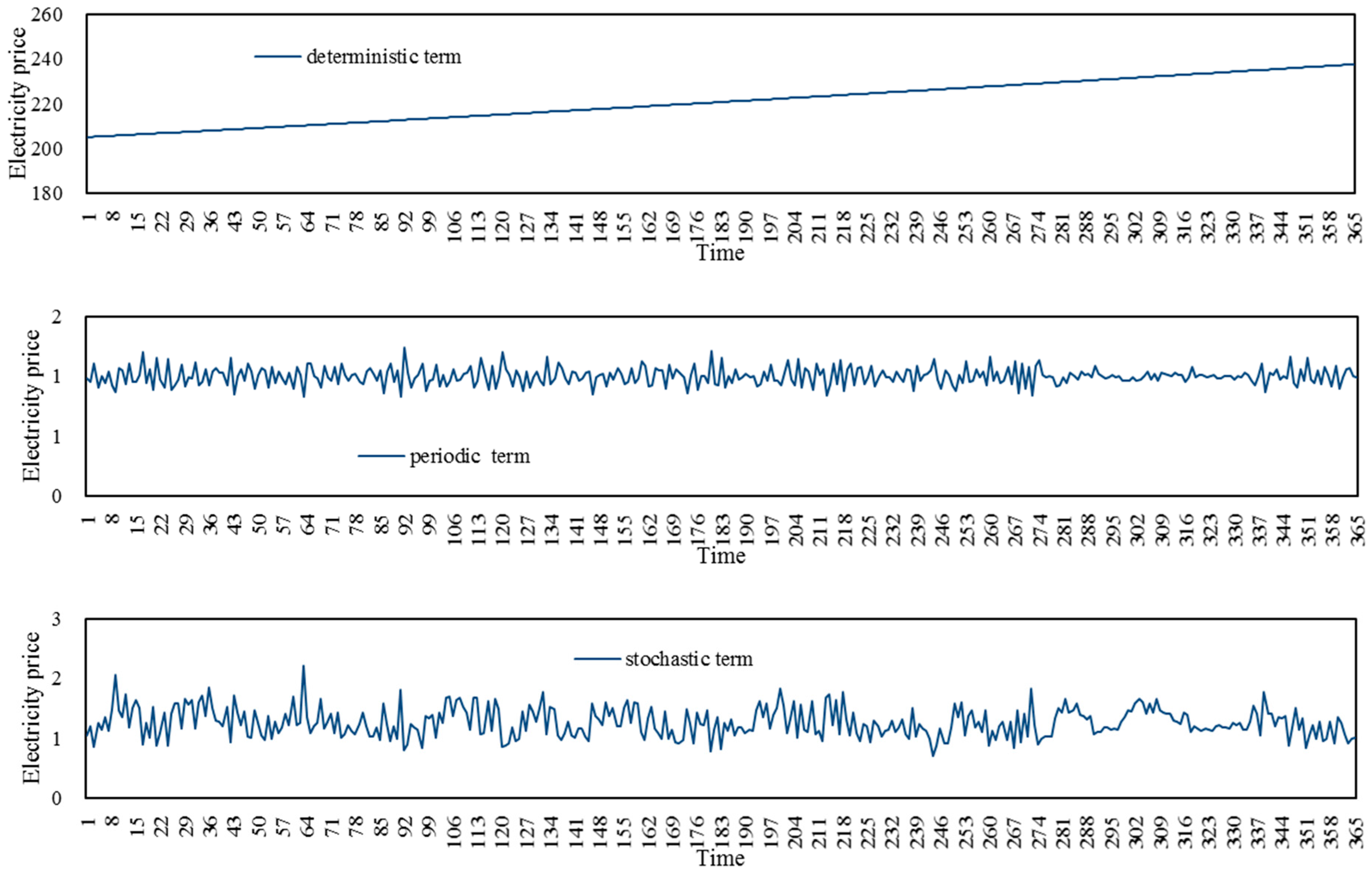
The BND method is firstly used to decompose the logarithmic sequence of daily electricity price time series. Before decomposition, it should do unit root test based on ADF test to judge whether the logarithmic sequences of daily electricity price time series are first order stationary or not. The ADF test result is listed in Table 1, which indicates the time series of daily electricity price are stable after first order difference. So, the daily electricity price can be decomposed by using BND method, and the results are shown in Figure 3, which includes deterministic term, periodic term, and stochastic term.
4.2. FOA-LSSVM Forecasting Results
The FOA-LSSVM model is used to forecast these three decomposed terms, respectively. Two parameters of LSSVM model will be automatically determined by FOA. The inputs of FOA-LSSVM model for electricity price forecasting include historical electricity price at the same day of last month and electricity price yesterday and the day before yesterday. That is to say, for the deterministic term forecasting, the deterministic term at the same day of last month, yesterday and the day before yesterday will be treated as the input variables of the FOA-LSSVM-based electricity price forecasting model; for the periodic term forecasting, the periodic term at the same day of last month, yesterday and the day before yesterday will be treated as the input variables of the FOA-LSSVM-based model; for the stochastic term forecasting, the stochastic term at the same day of last month, yesterday and the day before yesterday will be treated as the input variables of the FOA- LSSVM-based model. Finally, the electricity price forecasting values can be obtained via the multiplication of the forecasted deterministic term, periodic term, and stochastic term.
Before using the FOA-LSSVM model to forecast, the sample data should be normalized by using Equation (29).
where xmin and xmax represent the minimum and maximum value of each input data series, respectively.
At the training stage, the parameters c and σ will be dynamically determined by FOA for the deterministic term, periodic term, and stochastic term, respectively, and the results are listed in Table 2. The iterative RMSE trends of FOA-LSSVM model for parameters optimization in terms of deterministic term, periodic term, and stochastic term are respectively shown in Figure 4. These optimal parameters values will be used for deterministic term forecasting, periodic term forecasting, and stochastic term forecasting at testing stage, and the forecasting results of deterministic term, periodic term, and stochastic term at testing stage, namely, daily electricity price between 1 September and 31 December, can be obtained. Finally, by multiplying the forecasted deterministic term, periodic term, and stochastic term from 1 September and 31 December, the electricity price from 1 September and 31 December can be obtained, which are shown in Figure 5.
5. Discussions
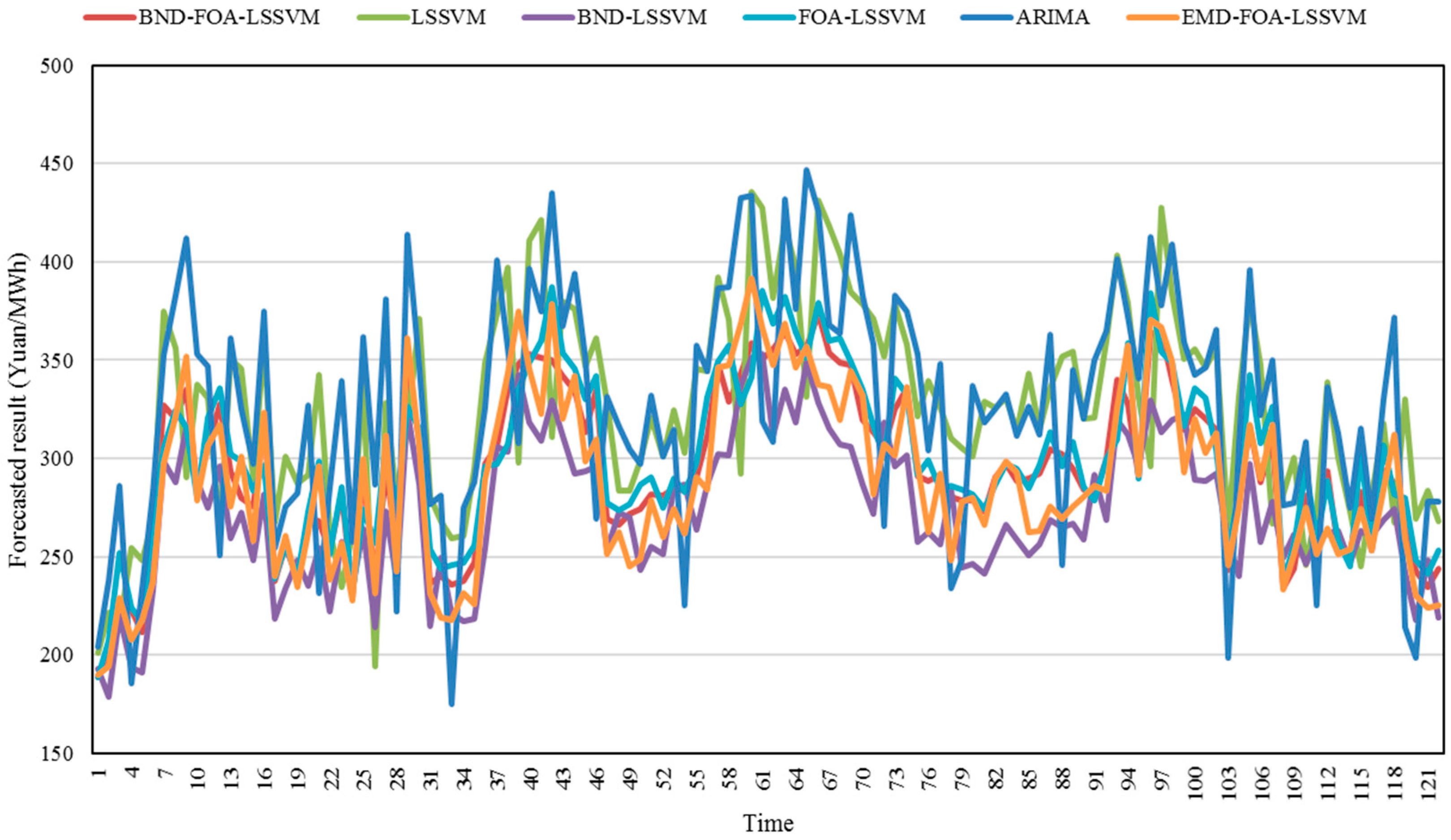
To verify the effectiveness of the proposed BND-FOA-LSSVM model for electricity price forecasting, five compared prediction models are selected in this paper, which are single LSSVM, BND-LSSVM, FOA-LSSVM, ARIMA (autoregressive integrated moving average), and EMD (empirical mode decomposition)-FOA-LSSVM. For single LSSVM model, there are no electricity price time series decomposition or parameter optimization. For the BND-LSSVM model, there is electricity price time series decomposition by using the BND method, but no parameter optimization. For the FOA-LSSVM model, there is parameter optimization by using FOA, but no electricity price time series decomposition. For ARIMA, there is no electricity price time series decomposition. For the EMD-FOA-LSSVM model, the electricity price time series are firstly decomposed into deterministic term, periodic term, and stochastic term, and then these three terms will be separately forecasted by using the FOA-LSSVM model. For single LSSVM, BND-LSSVM, FOA-LSSVM, and EMD-FOA-LSSVM models, the input variables, output variable and related parameters are set as the same as that in Section 4. For the ARIMA model, the daily electricity price data is served as input variable.
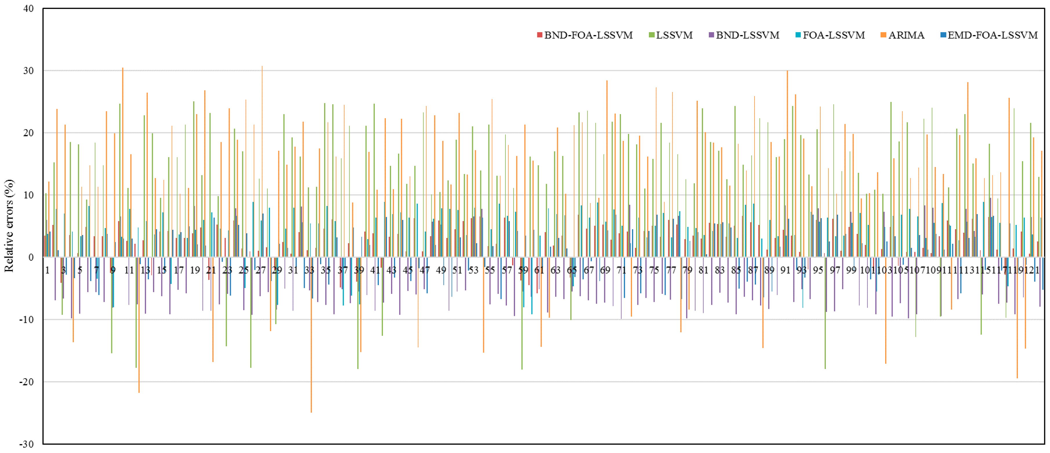
The electricity price forecasting results of the proposed BND-FOA-LSSVM, single LSSVM, BND-LSSVM, FOA-LSSVM, ARIMA and EMD-FOA-LSSVM models are shown in Figure 6, and the relative errors of forecasted electricity price by using these six models are listed in Figure 7. From Figure 7, it can be seen that all the relative errors of forecasted electricity price of the proposed BND-FOA-LSSVM model are smaller than 6.8%, and some are even smaller than 1%, such as 5 September, 26 September, 1 October, 15 October, 17 October, 2 December, 5 December, 15 December, 16 December, 18 December, and 30 December. However, the relative errors of forecasted electricity price of single LSSVM and ARIMA models are much larger, and some are more than 20%. The maximum and minimum relative errors of BND-LSSVM model are, respectively, −9.88% and 4.14%, and those of FOA-LSSVM model are, respectively, −9.13% and 2.26%. The maximum and minimum relative errors of EMD-FOA-LSSVM model are, respectively, 7% and 0.48%. Therefore, it can be said that, from the perspective of relative error, the proposed BND-FOA-LSSVM model has the best electricity price forecasting performance.
To further verify the forecasting performance of the proposed BND-FOA-LSSVM model, three frequently used forecasting error criteria are also selected, namely root mean square error (RMSE, as shown in Equation (27)), mean absolute percentage error (MAPE, as shown in Equation (30)), and mean absolute error (MAE, as shown in Equation (31)).
where is actual value of electricity price at time k; is forecasting value of electricity price at time k.
The RMSEs, MAPEs and MAEs of these six forecasting models, namely, BND-FOA-LSSVM, LSSVM, BND-LSSVM, FOA-LSSVM, ARIMA and EMD-FOA-LSSVM, are listed in Table 3. From the perspective of RMSE, the proposed BND-FOA-LSSVM model has the best forecasting performance because it has the minimum RMSE (namely 11.18 Yuan/MWh), followed by the EMD-FOA-LSSVM, FOA-LSSVM, BND-LSSVM, LSSVM, and ARIMA models. The RMSE of the BND-FOA-LSSVM model is (12.06 − 11.18)/12.06 = 7.30%, (18.05 − 11.18)/18.05 = 38.06%, (21.36 − 11.18)/21.36 = 47.66%, (50.78 − 11.18)/50.78 = 77.98%, and (53.43 − 11.18)/53.43 = 79.08% lower than that of the EMD-FOA-LSSVM, FOA-LSSVM, BND-LSSVM, LSSVM, and ARIMA models, respectively. From the perspective of MAPE, the proposed BND-FOA-LSSVM model still has the minimum MAPE value, which is 3.48%, much lower than that of the LSSVM, BND-LSSVM, FOA-LSSVM, ARIMA, and EMD-FOA-LSSVM models. The MAPE of the BND-FOA-LSSVM model is (3.76 − 3.48)/3.76 = 7.45%, (5.84 − 3.48)/5.84 =40.41%, (7.27 − 3.48)/7.27 = 52.13%, (16.89 − 3.48)/16.89 = 79.40%, and (17.71 − 3.48)/17.71 = 80.35% lower than that of EMD-FOA-LSSVM, FOA-LSSVM, BND-LSSVM, LSSVM, and ARIMA models, respectively. Meanwhile, the proposed BND-FOA-LSSVM model obtains the minimum MAE, which is 9.95 Yuan/MWh. The MAE of the BND-FOA-LSSVM model is (10.81 − 9.95)/10.81 = 7.96%, (16.92 − 9.95)/16.92 = 41.19%, (20.82 − 9.95)/20.82 = 52.21%, (48.50 − 9.95)/48.50 = 79.48%, and (50.63 − 9.95)/50.63 = 80.35% lower than that of the EMD-FOA-LSSVM, FOA-LSSVM, BND-LSSVM, LSSVM, and ARIMA models, respectively.
Therefore, it can be concluded that the proposed BND-FOA-LSSVM model has the best forecasting performance for electricity price forecasting because it has the minimum MAPE, RMSE and MAE. The EMD-FOA-LSSVM model also obtain high forecasting accuracy, but lower than that of the BND-FOA-LSSVM model, which indicates that the BND is an effective time series decomposition technique. The ARIMA model obtains the worst forecasting performance related to electricity price because it has the maximum MAPE, RMSE and MAE. The single LSSVM model has better electricity price forecasting performance compared with ARIMA model, which indicates the superiority of machine learning technique related to electricity price forecasting. The BND-LSSVM model has better electricity price forecasting performance compared with the single LSSVM model, which indicates the BND is an effective time series decomposition method because it can improve the forecasting accuracy. The FOA-LSSVM model has better forecasting performance compared with the BND-LSSVM model and the LSSVM model, which indicates the FOA is an efficient parameter optimization technique for LSSVM model related to electricity price forecasting because it can improve the forecasting accuracy of electricity price.
All in all, the proposed BND-FOA-LSSVM model is effective and practical for electricity price forecasting, which can improve the forecasting accuracy of electricity price.
6. Conclusions
In this paper, a new novel hybrid electricity price forecasting model based on BND-FOA-LSSVM was proposed. The electricity price time series are first decomposed into deterministic term, periodic term, and stochastic term. Then, these three decomposed terms are respectively forecasted by using the FOA-LSSVM model, and two parameters of the LSSVM model are automatically determined by using the FOA algorithm. Finally, the forecasting result of electricity price can be obtained by multiplying the forecasted deterministic term, periodic term, and stochastic term. The case study and forecasting performance evaluation indicate the proposed the BND-FOA-LSSVM model has the best forecasting performance compared with single LSSVM, BND-LSSVM, FOA-LSSVM, ARIMA, and EMD-FOA-LSSVM models for electricity price forecasting. The MAPE, RMSE and MAE of BND-FOA-LSSVM model are, respectively, 3.48%, 11.18 Yuan/MWh and 9.95 Yuan/MWh, which are much smaller than that of the LSSVM, BND-LSSVM, FOA-LSSVM, ARIMA, and EMD-FOA-LSSVM models. The proposed BND-FOA-LSSVM model for electricity price forecasting in this paper is effective and practical, which enriches the methodology library of electricity price forecasting. Meanwhile, the proposed method in this paper can also be used for other issues, such as power load forecasting, renewable energy forecasting, and economic forecasting.
Author Contributions
Weishang Guo conceived and performed the experiments, and wrote the paper; Zhenyu Zhao analyzed the data. Both authors have read and approved the final version.
Conflicts of Interest
The authors declare no conflict of interest.
References
- Panapakidis, I.P.; Dagoumas, A.S. Day-ahead electricity price forecasting via the application of artificial neural network based models. Appl. Energy 2016, 172, 132–151. [Google Scholar] [CrossRef]
- Weron, R. Electricity price forecasting: A review of the state-of-the-art with a look into the future. Int. J. Forecast. 2014, 30, 1030–1081. [Google Scholar] [CrossRef]
- Mandal, P.; Srivastava, A.K.; Senjyu, T.; Negnevitsky, M. Electricity Price Forecasting Using Neural Networks and Similar Days. Adv. Electr. Power Energy Syst. Load Price Forecast. 2017, 215. [Google Scholar] [CrossRef]
- Nowotarski, J.; Weron, R. On the importance of the long-term seasonal component in day-ahead electricity price forecasting. Energy Econom. 2016, 57, 228–235. [Google Scholar] [CrossRef]
- Portela, J.; Munoz, A.; Alonso, E. Forecasting functional time series with a new Hilbertian ARMAX model: Application to electricity price forecasting. IEEE Trans. Power Syst. 2017. [Google Scholar] [CrossRef]
- Yang, Z.; Ce, L.; Lian, L. Electricity price forecasting by a hybrid model, combining wavelet transform, ARMA and kernel-based extreme learning machine methods. Appl. Energy 2017, 190, 291–305. [Google Scholar] [CrossRef]
- Gao, G.; Lo, K.; Fan, F. Comparison of ARIMA and ANN models used in electricity price forecasting for power market. Energy Power Eng. 2017, 9, 120–126. [Google Scholar] [CrossRef]
- Nowotarski, J.; Weron, R. Recent advances in electricity price forecasting: A review of probabilistic forecasting. Renew. Sustain. Energy Rev. 2017. [Google Scholar] [CrossRef]
- Huang, Y.-S.; Huang, S.-H.; Hu, Y.-P. Short-Term Electricity Price Forecasting Based on Nonparametric GARCH Residuals Correction-Least Square Support Vector Machine. In Management Information and Optoelectronic Engineering, Proceedings of the 2016 International Conference on Management, Information and Communication (ICMIC2016) and the 2016 International Conference on Optics and Electronics Engineering (ICOEE2016), Guilin, China, 28–29 May 2016; World Scientific: Singapore, 2017; pp. 42–48. [Google Scholar]
- Girish, G. Spot electricity price forecasting in Indian electricity market using autoregressive-GARCH models. Energy Strategy Rev. 2016, 11, 52–57. [Google Scholar] [CrossRef]
- Cifter, A. Forecasting electricity price volatility with the Markov-switching GARCH model: Evidence from the Nordic electric power market. Electric Power Syst. Res. 2013, 102, 61–67. [Google Scholar] [CrossRef]
- Keles, D.; Scelle, J.; Paraschiv, F.; Fichtner, W. Extended forecast methods for day-ahead electricity spot prices applying artificial neural networks. Appl. Energy 2016, 162, 218–230. [Google Scholar] [CrossRef]
- Monteiro, C.; Ramirez-Rosado, I.J.; Fernandez-Jimenez, L.A.; Conde, P. Short-Term Price Forecasting Models Based on Artificial Neural Networks for Intraday Sessions in the Iberian Electricity Market. Energies 2016, 9, 721. [Google Scholar] [CrossRef]
- Amjady, N. Day-ahead price forecasting of electricity markets by a new fuzzy neural network. IEEE Trans. Power Syst. 2006, 21, 887–896. [Google Scholar] [CrossRef]
- Chen, X.; Dong, Z.Y.; Meng, K.; Xu, Y.; Wong, K.P.; Ngan, H. Electricity price forecasting with extreme learning machine and bootstrapping. IEEE Trans. Power Syst. 2012, 27, 2055–2062. [Google Scholar] [CrossRef]
- Shrivastava, N.A.; Panigrahi, B.K. A hybrid wavelet-ELM based short term price forecasting for electricity markets. Int. J. Electr. Power Energy Syst. 2014, 55, 41–50. [Google Scholar] [CrossRef]
- Sansom, D.C.; Downs, T.; Saha, T.K. Evaluation of support vector machine based forecasting tool in electricity price forecasting for Australian national electricity market participants. J. Electr. Electron. Eng. Aust. 2003, 22, 227–233. [Google Scholar]
- Yan, X.; Chowdhury, N.A. Mid-term electricity market clearing price forecasting: A multiple SVM approach. Int. J. Electr. Power Energy Syst. 2014, 58, 206–214. [Google Scholar] [CrossRef]
- Catalão, J.P.S.; Pousinho, H.M.I.; Mendes, V.M.F. Hybrid wavelet-PSO-ANFIS approach for short-term electricity prices forecasting. IEEE Trans. Power Syst. 2011, 26, 137–144. [Google Scholar] [CrossRef]
- Pousinho, H.M.I.; Mendes, V.M.F.; Catalão, J.P.S. Short-term electricity prices forecasting in a competitive market by a hybrid PSO–ANFIS approach. Int. J. Electr. Power Energy Syst. 2012, 39, 29–35. [Google Scholar] [CrossRef]
- Huang, S.; Han, Y.; Liu, F.; Song, J. Weights Optimization Based on Genetic Algorithm for Variable Weight Combination Model of BP-LSSVM for Day-ahead Electricity Price Forecasting. DEStech Trans. Comput. Sci. Eng. 2016. [Google Scholar] [CrossRef]
- Alamaniotis, M.; Bargiotas, D.; Bourbakis, N.G.; Tsoukalas, L.H. Genetic optimal regression of relevance vector machines for electricity pricing signal forecasting in smart grids. IEEE Trans. Smart Grid 2015, 6, 2997–3005. [Google Scholar] [CrossRef]
- Guo, Z.; Zhao, J.; Zhang, W.; Wang, J. A corrected hybrid approach for wind speed prediction in Hexi Corridor of China. Energy 2011, 36, 1668–1679. [Google Scholar] [CrossRef]
- Zhu, B.; Wei, Y. Carbon price forecasting with a novel hybrid ARIMA and least squares support vector machines methodology. Omega 2013, 41, 517–524. [Google Scholar] [CrossRef]
- Kaytez, F.; Taplamacioglu, M.C.; Cam, E.; Hardalac, F. Forecasting electricity consumption: A comparison of regression analysis, neural networks and least squares support vector machines. Int. J. Electr. Power Energy Syst. 2015, 67, 431–438. [Google Scholar] [CrossRef]
- Li, H.; Guo, S.; Zhao, H.; Su, C.; Wang, B. Annual electric load forecasting by a least squares support vector machine with a fruit fly optimization algorithm. Energies 2012, 5, 4430–4445. [Google Scholar] [CrossRef]
- Peng, T.; Tang, Z. A small scale forecasting algorithm for network traffic based on relevant local least squares support vector machine regression model. Appl. Math 2015, 9, 653–659. [Google Scholar]
- Yu, Y.; Li, Y.; Li, J.; Gu, X. Self-adaptive step fruit fly algorithm optimized support vector regression model for dynamic response prediction of magnetorheological elastomer base isolator. Neurocomputing 2016, 211, 41–52. [Google Scholar] [CrossRef]
- Yu, Y.; Li, Y.; Li, J. Parameter identification and sensitivity analysis of an improved LuGre friction model for magnetorheological elastomer base isolator. Meccanica 2015, 50, 2691–2707. [Google Scholar] [CrossRef]
- Beveridge, S.; Nelson, C.R. A new approach to decomposition of economic time series into permanent and transitory components with particular attention to measurement of the ‘business cycle’. J. Monetary Econ. 1981, 7, 151–174. [Google Scholar] [CrossRef]
- Guo, S.; Zhao, H.; Zhao, H. A New Hybrid Wind Power Forecaster Using the Beveridge-Nelson Decomposition Method and a Relevance Vector Machine Optimized by the Ant Lion Optimizer. Energies 2017, 10, 922. [Google Scholar] [CrossRef]
- Nelson, C.R.; Plosser, C.R. Trends and random walks in macroeconmic time series: Some evidence and implications. J. Monetary Econ. 1982, 10, 139–162. [Google Scholar] [CrossRef]
- Morley, J.C. A state–space approach to calculating the Beveridge–Nelson decomposition. Econ. Lett. 2002, 75, 123–127. [Google Scholar] [CrossRef]
- Pan, W.-T. A new fruit fly optimization algorithm: Taking the financial distress model as an example. Knowl.-Based Syst. 2012, 26, 69–74. [Google Scholar] [CrossRef]
- Li, H.-Z.; Guo, S.; Li, C.-J.; Sun, J.-Q. A hybrid annual power load forecasting model based on generalized regression neural network with fruit fly optimization algorithm. Knowl.-Based Syst. 2013, 37, 378–387. [Google Scholar] [CrossRef]
- Pan, W.-T. Mixed modified fruit fly optimization algorithm with general regression neural network to build oil and gold prices forecasting model. Kybernetes 2014, 43, 1053–1063. [Google Scholar] [CrossRef]
- Li, M.-W.; Geng, J.; Han, D.-F.; Zheng, T.-J. Ship motion prediction using dynamic seasonal RvSVR with phase space reconstruction and the chaos adaptive efficient FOA. Neurocomputing 2016, 174, 661–680. [Google Scholar] [CrossRef]
- Suykens, J.A.; Van Gestel, T.; De Brabanter, J. Least Squares Support Vector Machines; World Scientific: Singapore, 2002. [Google Scholar]
- Suykens, J.A.; Vandewalle, J. Least squares support vector machine classifiers. Neural Process. Lett. 1999, 9, 293–300. [Google Scholar] [CrossRef]
Figure 1.
Flowchart of the proposed Beveridge-Nelson decomposition (BND)-fruit fly optimization algorithm (FOA)-least square support vector machine (LSSVM) model for electricity price forecasting.
Figure 1.
Flowchart of the proposed Beveridge-Nelson decomposition (BND)-fruit fly optimization algorithm (FOA)-least square support vector machine (LSSVM) model for electricity price forecasting.
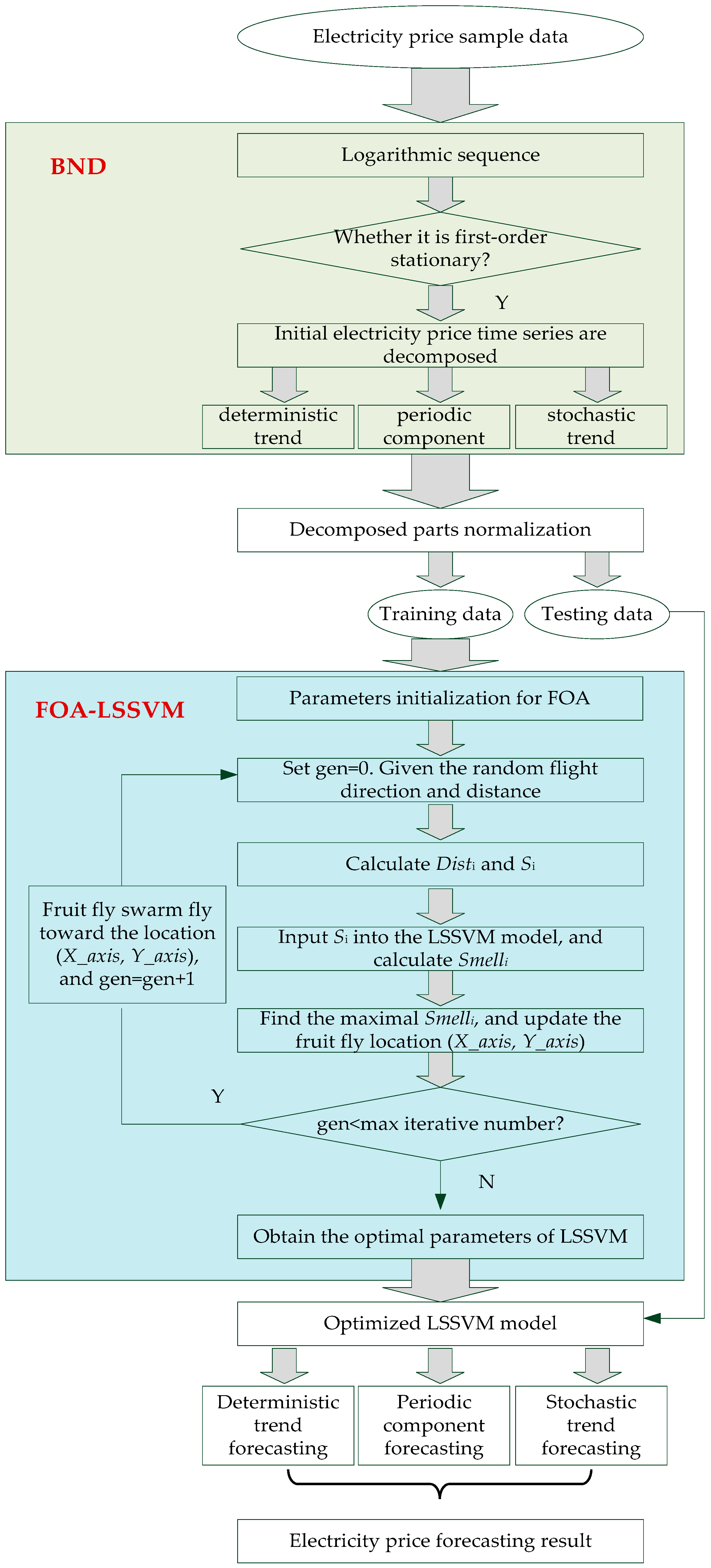
Figure 2.
Daily electricity price time series from 1 January to 31 December.

Figure 3.
Decomposed deterministic term, periodic term, and stochastic term of original daily electricity price time series.
Figure 3.
Decomposed deterministic term, periodic term, and stochastic term of original daily electricity price time series.

Figure 4.
The iterative RMSE trends of FOA-LSSVM model for deterministic term, periodic term, and stochastic term.
Figure 4.
The iterative RMSE trends of FOA-LSSVM model for deterministic term, periodic term, and stochastic term.
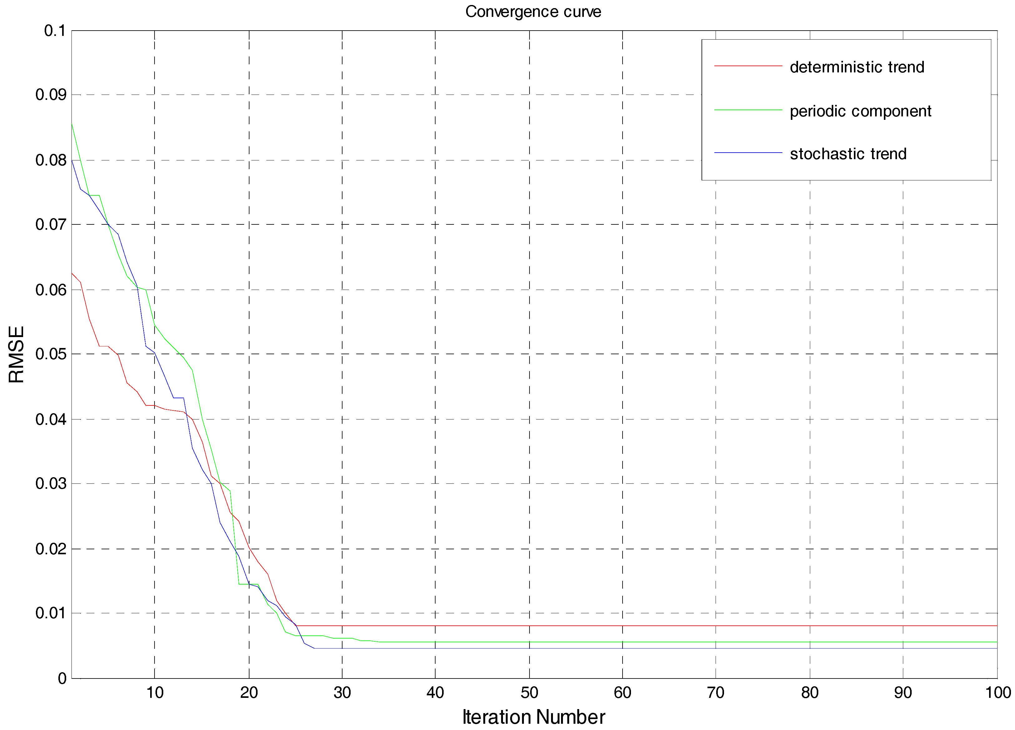
Figure 5.
Forecasting result of electricity price from 1 September and 31 December.

Figure 6.
Forecasting results of electricity price from 1 September and 31 December by using different methods.
Figure 6.
Forecasting results of electricity price from 1 September and 31 December by using different methods.

Figure 7.
Relative errors of electricity price forecasting of different models (Unit: %).


Table 1.
The Augmented Dickey-Fuller (ADF) test results.
| Sequence | Test Form (C,T,K) | ADF Test Value | p Value | Conclusion |
|---|---|---|---|---|
| (N,N,1) | −1.5398 | 0.1958 | Unstable | |
| (N,N,0) | −10.6845 | 0.0000 | stable |
Table 2.
The optimal values of σ2 and c.
| Parameters | Deterministic Trend | Periodic Component | Stochastic Trend |
|---|---|---|---|
| σ2 | 3.2174 | 3.0478 | 4.5733 |
| c | 16.5741 | 10.5822 | 12.9847 |
Table 3.
Forecasting performances of different methods. Auto-regressive integrated moving average (ARIMA); empirical mode decomposition (EMD); mean absolute percentage error (MAPE); root mean square error (RMSE); mean absolute error (MAE).
Table 3.
Forecasting performances of different methods. Auto-regressive integrated moving average (ARIMA); empirical mode decomposition (EMD); mean absolute percentage error (MAPE); root mean square error (RMSE); mean absolute error (MAE).
| Error Criteria | BND-FOA-LSSVM | LSSVM | BND-LSSVM | FOA-LSSVM | ARIMA | EMD-FOA-LSSVM |
|---|---|---|---|---|---|---|
| RMSE (Yuan/MWh) | 11.18 | 50.78 | 21.36 | 18.05 | 53.43 | 12.06 |
| MAPE (%) | 3.48 | 16.89 | 7.27 | 5.84 | 17.71 | 3.76 |
| MAE (Yuan/MWh) | 9.95 | 48.50 | 20.82 | 16.92 | 50.63 | 10.81 |
© 2017 by the authors. Licensee MDPI, Basel, Switzerland. This article is an open access article distributed under the terms and conditions of the Creative Commons Attribution (CC BY) license (http://creativecommons.org/licenses/by/4.0/).
Share and Cite
MDPI and ACS Style
Guo, W.; Zhao, Z. A Novel Hybrid BND-FOA-LSSVM Model for Electricity Price Forecasting. Information 2017, 8, 120. https://doi.org/10.3390/info8040120
AMA Style
Guo W, Zhao Z. A Novel Hybrid BND-FOA-LSSVM Model for Electricity Price Forecasting. Information. 2017; 8(4):120. https://doi.org/10.3390/info8040120
Chicago/Turabian StyleGuo, Weishang, and Zhenyu Zhao. 2017. "A Novel Hybrid BND-FOA-LSSVM Model for Electricity Price Forecasting" Information 8, no. 4: 120. https://doi.org/10.3390/info8040120
Note that from the first issue of 2016, this journal uses article numbers instead of page numbers. See further details here.