Efficient Data Collection by Mobile Sink to Detect Phenomena in Internet of Things

1
Department of Computer Science, University of Sharjah, P.O. Box 27272 Sharjah, UAE
2
Department of Electrical & Computer Engineering, University of Sharjah, P.O. Box 27272 Sharjah, UAE
*
Author to whom correspondence should be addressed.
Information 2017, 8(4), 123; https://doi.org/10.3390/info8040123
Submission received: 13 September 2017
/
Revised: 25 September 2017
/
Accepted: 28 September 2017
/
Published: 3 October 2017
Abstract
:With the rapid development of Internet of Things (IoT), more and more static and mobile sensors are being deployed for sensing and tracking environmental phenomena, such as fire, oil spills and air pollution. As these sensors are usually battery-powered, energy-efficient algorithms are required to extend the sensors’ lifetime. Moreover, forwarding sensed data towards a static sink causes quick battery depletion of the sinks’ nearby sensors. Therefore, in this paper, we propose a distributed energy-efficient algorithm, called the Hilbert-order Collection Strategy (HCS), which uses a mobile sink (e.g., drone) to collect data from a mobile wireless sensor network (mWSN) and detect environmental phenomena. The mWSN consists of mobile sensors that sense environmental data. These mobile sensors self-organize themselves into groups. The sensors of each group elect a group head (GH), which collects data from the mobile sensors in its group. Periodically, a mobile sink passes by the locations of the GHs (data collection path) to collect their data. The collected data are aggregated to discover a global phenomenon. To shorten the data collection path, which results in reducing the energy cost, the mobile sink establishes the path based on the order of Hilbert values of the GHs’ locations. Furthermore, the paper proposes two optimization techniques for data collection to further reduce the energy cost of mWSN and reduce the data loss.
1. Introduction
The Internet of Things (IoT) is emerging as a new computing paradigm that connects uniquely identifiable objects (sensing devices) to an internet-like network. IoT is the natural continuity of the ambient intelligence where a large number of sensing devices are interconnected to detect and track the environment [1]. These sensing devices are either static or mobile sensors and usually form a network and collectively monitor environmental phenomena, such as fire, oil spills, and poisonous gases [2,3] Sensors’ data could be used in other applications such as habitat monitoring [4,5], undersea monitoring [6], battlefield observation [7], and industrial safety and control [8]. Typically, the sensors communicate wirelessly and thus form a wireless sensor network. As these sensors are usually battery-powered, energy-efficient algorithm design is required to extend the network’s lifetime [9].
This paper proposes a distributed energy-efficient data collection strategy, called the Hilbert-order Collection Strategy (HCS), to collect environmental data using a mobile wireless sensor network (mWSN) and detect possible phenomena. The mobile sensors of mWSN (i.e., mobile phones or taxis) self-organize themselves into groups and then the sensors of each group elect a group head (GH). Typically, a GH is a sensor with the maximum remaining power in the group. Each GH collects the sensed data from sensors in its group at the beginning of every time window, w, and then processes the collected data to detect possible local phenomena within the geographical boundary of the group. Traditionally, collected data by GHs can be reported to a static sink in one hop if the environment is a small geographical region. In relatively big environments, multi-hop routing to a static sink is used; however, this may lead to congestion at sensors around the static sink. As a result, these sensors suffer from high-energy drainage, which disrupts the flow of data to the sink [10]. To alleviate this problem, a mobile sink is proposed to collect the groups’ data from GHs.
In the proposed HCS, the groups’ data are collected by a mobile sink (i.e., drone) that passes by the locations of GHs. Then, the collected data is processed to discover possible global phenomena. The mobile sink visits all GHs in a specific order, called data collection path, to collect their data. The mobile sink enters the field that contains the GHs once every τ—duration, which is termed the trip time, to collect data from GHs. It is essential that the trip time τ is less than, or equal to, the time window w. Note that the time window w is the time taken by GHs to collect data from the mobile sensors within their groups, process the data and then wait for the mobile sink to pass by to collect the data. This suggests that a mobile sink should carefully plan its path to visit all GHs in the shortest time possible. Hence, the proposed HCS forms the data collection path based on the Hilbert-order of the GHs’ locations. Hilbert order of GHs’ locations provides an overall short data collection path for the mobile sink as compared to orders of GHs given by other space filling curves as shown by our experiments.
The paper also proposes two optimization techniques for data collection, called Phenomena-aware Collection Technique (PCT) and Lazy Update Technique (LUT), to further reduce the data loss and energy cost of the mWSN. PCT reduces the number of GHs that form the data collection path to only those GHs that detected local phenomena and therefore the data collection path is shortened. As a result, the trip time τ is reduced, which results in reducing the data loss. On the other hand, LUT proposes to update the data collection path every nth windows, where n > 1, instead of being updated every window. That is the overhead of selecting new GHs and forming a new data collection path is delayed, which reduces the overall energy cost of mWSN.
To evaluate the proposed HCS algorithm, we developed a new energy model. The proposed HCS algorithm and optimization techniques are validated using a comprehensive set of experiments implemented on NS2 network simulator.
The main contributions of this paper are summarized as follows:
- A distributed energy-efficient algorithm, called Hilbert-order data collection strategy (HCS), to collect environmental data and detect possible phenomena. HCS method uses Hilbert-order method to compute the data collection path of the mobile sink.
- Two data collection optimization techniques, namely Phenomena-aware Collection Technique (PCT) and Lazy Update Technique (LUT), to reduce the data loss and overall energy cost of the network.
- An energy model for the proposed mobile wireless sensor network.
The rest of the paper is organized as follows. In Section Section 2, we review the related work. Section Section 3 presents a formal definition of phenomena detection in mWSN and outlines the proposed solution. The proposed HCS algorithm and the optimization techniques, PCS and LUT, are presented in Section 4. In Section 5, we present the energy cost model of the proposed approach. Section 6 presents our simulation experiments. Finally, Section 7 concludes the paper.
2. Related Work
IoT has been recently used to intelligently monitor the environment. Using a large number of sensing devices that are interconnected, environment information is sensed and reported to a sink to detect and track phenomena [1]. Detecting phenomena using sensor networks has received the attention of many researchers in the data mining community. In this section, we survey the related work of phenomena detection by sensor networks.
2.1. Detecting Environmental Phenomena
Several research works were conducted to detect outliers in data streams produced by wireless sensor networks (WSNs). The problem of detecting phenomena using deployed sensors is defined as the detection of outliers in the collected sensor’s data [11]. Rajasegarar et al. [12] propose a cluster-based global outlier detection technique. This approach reduces the communication overhead between sensors and the sink by summarizing the data at the cluster head and then reporting summaries to the sink rather than raw sensor measurements. In [13], a static WSN collects and reports Discrete Fourier Transformation representations of the data streams to reduce the dimensionality of the streams. Then, a grid based clustering technique is used to detect phenomena. The work in [2] improved the system in [13] by using a distributed scheme to reduce the energy cost of the WSN; however, both systems consider static nodes and static sink. The work in [14] proposed a cluster-based system for distributed event detection. A similar system proposed by [15] in which sensors are divided into cells based on their location. Each cell has a group head that collects the data from the sensors within the cell. An event is detected by matching the collected data with a template grid. Sheng et al. [16] presented a histogram-based technique to identify global outliers. To reduce the communication overhead, a nearest neighbor-based approach was proposed by the authors of [17], in which each sensor uses similarity function to detect local anomalies and then send detected outliers to neighboring nodes for verification. The above systems only consider static sensors.
Few research works address the problem of gathering data in mobile sensor networks by a mobile sink. For example, Liu et al. [18] minimize the energy consumption of data gathering in mobile WSN by first electing group head and then cluster data using a mechanism called (Clustering with Mobility) CM. In [19,20], the authors discussed the effects of various group formation mechanisms in mobile sensor networks using a Simple Mobility model. Davies [21] used a Random Walk Mobility model where a sensor node can randomly choose a speed within a given range and a direction to move. Random Direction Mobility model was suggested by Royer et al. [22], in which each sensor has a constant speed and can randomly choose a direction to travel.
2.2. Mobile Sinks in WSN
Recent research studies have focused on collecting data using mobile sinks to reduce congestions at sensors around the static sink. However, a critical issue that should be addressed is the delay in data collection, which causes data loss.
The authors of [23] proposed a tree-based heuristics topology control algorithm to maximize the lifetime of WSNs with mobile sinks. Within a predefined delay tolerance level, each node does not need to send the data immediately as it becomes available. Instead, a node can store data temporarily and transmit it when the mobile sink arrives at the most favorable location. In [10], a framework is presented to study the impacts of multi-hop packet routing in WSNs with mobile sinks. Cluster heads buffer the received data until the mobile data harvester contacts it. A ring structure is propose by [24] to provide load-balanced data delivery and achieve uniform-energy consumption across the network. To reduce load on the ring nodes, each ring node independently selects new ring nodes among their neighbors when their batteries nears dying, while conserving the closed loop and the encapsulation of the network center properties. The drawback of Ring Routing is its scalability on larger scale WSN. Recently, some researchers computed the shortest data collection path for a mobile sink such as the Traveling Salesman Problem, TSP [25,26]. Although TSP based methods produce a short traveling path for the mobile sink, they require calculation of a distance matrix (distances between all the nodes), which is one of the largest drawbacks of TSP implementation. The work in [27] proposed a mobile sink routing strategy for a network based on a combined time-driven and event-driven pattern, which periodically transmits routine data to the sink. The authors of [28] proposed an approach to calculate an optimal sink path that takes into consideration the nodes distribution, which is effective in environments with unbalanced node distribution, however finding the optimal path requires high communication overhead. In [29], an approach to use a mobile sink to collect data from cluster representatives is proposed. The sink chooses its path based on the closest clusters’ representatives. The authors of [25] proposed a data collection scheme in which a mobile sink moves in the environment in an undetermined path and broadcast its location from time to time to all nodes. Although the paper shows a faster data delivery, the approach consume considerable amount of energy in forwarding the data—sometimes via multiple hops—to the location of the sink.
3. HCS Design Issues
In this section, we formulate the problem and outline the solution as well as important design issues, such as sink mobility, sensors’ mobility and time window.
3.1. Problem Formulation
The key problem addressed in this paper is to utilize IoT to detect environmental phenomena, such as fire, air pollution and oil spills. Given a mWSN, which is a set of mobile sensors S = {s1 + s2 + … + sNs}, where Ns is the total number of mobile sensors that sense data about the environment, the aim is to design an efficient algorithm to collect and process such data to detect environmental phenomena.
To maintain updated information about the phenomena, the proposed algorithm should collect and process the environment data periodically. That is once every time window w.
Definition 1:
(time window, w) is the time taken by GHs to collect data from the mobile sensors within their groups, process the data and then wait for the mobile sink, MS, to pass by to collect the data.
Where the time of w is decided by the urgency of the application. If we assume that each group of mobile sensors are moving in a certain region of the monitored field, then the proposed algorithm should collect the data from each group of mobile sensors. For example, let the monitored field be the city of Dubai, which consists of different regions, and in each region there are mobile sensors (i.e., sensors mounted on taxis, or mobile phones) sensing the environment, then a mobile sink MS should pass by these different groups to collect the data. Then, MS aggregates the data and detects the global environmental phenomena.
Definition 2:
(trip time, τ) is the time taken by MS pass by the GHs in the monitored field to collect the data of all groups.
Therefore, it is essential that w ≥ τ. The tradeoff is that as w is extended to be very large, the freshness of the collected data becomes low since the mobile sensors report their sensed data at the beginning of every window. However, if w is small, that is τ > w, then data loss might occur. That is because a new window starts before MS finishes its data collection and thus some mobile sensors will start collecting the new data that results in overwriting the collected data of the previous window. Thus, the proposed solution for phenomena detection, should balance the times of w and τ to avoid data loss. Moreover, to extend the lifetime of the mobile sensor network, the total energy cost ξtotal of the mWSN should be minimized.
3.2. Solution Outline
We propose Hilbert-order Collection Strategy, HCS, which is an energy-efficient data collection strategy to minimize the data loss and energy cost of the network. In HCS, mobile sensors self-organize themselves into groups and then the sensors of each group elect a GH. Each GH collects the sensed data from sensors in its group every time window, w, and then processes the data to detect possible local phenomena within the geographical boundary of the group. A MS passes by the locations of GHs to collect the group’s data, which is processed to discover possible global phenomena.
Thus, HCS shortens the data collection path of MS by ordering the locations of GHs by their Hilbert values. As a result, τ is reduced, which in turn reduces the data loss. Additionally, the paper proposes PCT and LUT, which are optimization techniques to further shorten the data collection path and greatly reduce the energy cost of the mWSN, respectively. PCT limits the number of GHs reporting the phenomena to those that detected the phenomena and LUT delays update of electing new GHs for the following window until the nth window instead of performing the update at the end of every window.
3.2.1. Sensor Mobility
Sensors move according to the Random Walk model within w, where a sensor randomly chooses a speed within a given range and direction at the beginning of every window wi. We assume that the sensor’s speed and direction are fixed within wi. However, the speed and direction of individual sensors may change in different windows. Within a window, different sensors may have different speeds and directions. The mobile sink travels according to the computed data collection path. We assume that the trip time, τ, of the mobile sink does not exceed the time allowed by its battery.
3.2.2. Time Window
Monitoring an environment means sensing continuously the surrounding area and reporting the sensed data. The reported data from each sensor is considered as an infinite data stream. Due to the characteristics of these data streams (infinite, continuous and high rate), a practical solution to detect phenomena from data streams is to divide the time dimension into time windows, w. The data corresponding to each window is processed and reported in the following phases (see Figure 1).
- Group Formation: mobile sensors associate themselves to the nearest GH.
- Local Phenomena Reporting: mobile sensors of each group report the observed phenomena data as well as their status information (remaining battery power, speed and direction) to their GH.
- GHs Election for Next Window: new set of GHs are elected for the next window based on their status and phenomena information.
- Data Collection by Mobile Sink: MS aggregates the collected local phenomena data to form a global phenomenon and computes the new data collection path for the next window.
The details of these phases will be discussed in Section 4.
3.2.3. Data Collection Path
In HCS, the Data Collection by Mobile Sink phase (see Figure 2), the MS computes a new data collection path of the next window based on the locations of the collected new set of GHs, which were computed by the current GHs. The MS uses a space-filling curve to create an optimized order of GHs to be visited in the next window. HCS uses the Hilbert-order values of the GHs’ spatial locations to compute the data collection path. The proximity property of the Hilbert-order results in a shorter data collection path. Hence, the data loss is greatly reduced. Note that data loss occurs when the trip time τ of MS is greater than the window time w.
The Hilbert-order value of a specific GH is determined based on its (x, y) location in a two-dimensional space [30]. Figure 2 shows an example of four group heads {A, B, C, D}. The space is a grid of size 4 × 4 cells. The Hilbert order of all groups will be computed by MS. The Hilbert-order value of GH A is formed by interleaving the value 01 of the x-coordinate and the value 10 of the y-coordinate. Thus, the Hilbert-order value of the group head A is (0111). Numbers in the cells of Figure 2 show the Hilbert-order value of each cell. In HCS, the data collection path of the MS is GH A, GH B, GH C and finally GH D. However, for HCS with PCT, the data collection path is GH A, GH B and GH C; that is the path only includes the GHs that detected the phenomena.
4. Phenomena Detection Using mWSN and MS
Given a set of mobile sensors S = {s1 + s2 + … + sNs}, where Ns is the total number of mobile sensors, we propose the HCS algorithm, which is a distributed energy-efficient algorithm to detect phenomena in an mWSN environment. Table 1 presents the descriptions of frequently used symbols that in the rest of the paper.
The proposed HCS that detects environmental phenomena has the following assumptions:
- The mobile sensors have prior knowledge of the normal range of values (non-phenomena values).
- The mobile sensors are homogenous; that is they have the same processing power, initial battery life, storage, and communication range.
- Individual mobile sensors may have different speeds and direction.
- The mobile sensors are all distributed on the ground of the monitored field, while the MS flies over at about equal height from GHs.
- GHs are normal mobile sensors.
Below we discuss the phases of the proposed HCS.
4.1. HCS for Phenomena Detection
At the beginning of every window, the new GHs announce themselves (broadcast their IDs) to the sensors in the environment. Then, each sensor associates itself to the closest GH; this is called Group Formation phase, see Figure 1. In the Local Phenomena Reporting phase, sensors that sensed phenomena report two types of information to their GHs: (1) sensed phenomena information; and (2) sensor status information (remaining battery power, speed and direction). Each GH collects the phenomena information from the sensors within its group and then it aggregates the collected information to discover local phenomena (phenomena within the boundaries of its group). In the third phase, GHs Election for Next Window, each current GH selects a GH for the next window based on the received status information of the sensors and the computed local phenomena location. That is, the new GH should have enough remaining power, and be located within the computed local phenomena as indicated by its speed and direction. Note that when the network is first deployed, the GHs in the initial window are selected randomly (this happens only once in the lifetime of the network). In the final phase, Data Collection by Mobile Sink, the MS passes by GHs to collect their local phenomena information as well as the elected new GHs for the next window. Then, MS joins the collected local phenomena information to form the global phenomena (phenomena in the whole environment), which is then sent to an application domain for further processing and tracking. Additionally, MS builds a new data collection path of the next window based on Hilbert order of the locations of the collected new set of GHs.
4.2. HCS Algorithm
In the HCS algorithm (see Algorithm 1), the GHs announce themselves as the new set of GHs by broadcasting their IDs (Lines 1–3) to all sensors in the environment. Then, each mobile sensors si associates itself with the closest GH (Lines 4–8) to minimize future communication costs. As a result, sensors are clustered into multiple disjoint groups. Each group has its own GH. Then, each sensor that observes a phenomenon, reports its phenomena observation, poi, as well as its status to its GH (Lines 9–14). The status of a sensor includes remaining battery power, speed and direction that will be used by the GH to select a GH for the next window. In line 15–20, each GH joins the collected phenomena observations (all poj) to detect local phenomena LPi. Also, each GH elects a new GH, GHinew, for the next window using the distributed group head election algorithm (DGH), which was proposed in [3]. In DGH, each current GH elects a new GH based on the on the sensors’ statuses (all ssj) and the computed local phenomena information, LPi. Thus, selection of the new set of GHs is based on the battery power, speed and direction. Thus, it is assumed that new GHs for the next window will be within the sensing range of all its members and be able to collect their data. In lines 21–24, every GHi report its LPi to MS. Additionally, every GHi reports the computed GH for the next window, GHinew, to MS. Note that GHs that did not detect local phenomena would remain as the GHs for the next window and thus would report themselves to MS among the GHinew. Then, MS joins all the collected local phenomena to create global phenomena GP (see line 25), which is sent to an application domain to further processing and tracking of the detected environmental phenomena. Then, in line 26, MS uses the GHinew to compute the data collection path for the next window. The data collection path is computed based on the Hilbert-order values of the spatial locations of all new GHs.
| Algorithm 1: HCS |
| Input: poi, ssi // poi is Phenomena observation, ssi is Sensor status. |
| Output: GP, DataCollPath // GP is global phenomena; DataCollPath is the computed data collection path for the next window. |
| 1: for each GHi in GHs do |
| 2: broadcastID(GHs) |
| 3: end for |
| 4: for each si in S do |
| 5: if s ∉ GHs |
| 6: AssociateWithClosestGH (GHs) |
| 7: end if |
| 8: end for |
| 9: for each si in S do |
| 10: if si sensed phenomenon |
| 11: reportObservationToGH (po, GH) |
| 12: reportStatusToGH (ss, GH) |
| 13: end if |
| 14: end for |
| 15: for each GHi in GHs do |
| 16: if GHi detected local phenomena |
| 17: LPi = computeLocalPhenomena (all poj) |
| 18: GHinew = electNewGHusingDGH (all ssj, LPi) |
| 19: end if |
| 20: end for |
| 21: for each GHi in GHs do |
| 22: reportLocalPhenomenaToSink (LPi, MS) |
| 23: reportNewGHsToSink (GHinew, MS) |
| 24: end for |
| 25: GP = computeGlobalPhenomena (all LPi) |
| 26: DataCollPath = computeDataCollectionPath (all GHinew) |
| 27: Return GP |
4.3. Optimizations of HCS
To increase the lifetime of the mWSN, we propose two optimization techniques for data collection to the proposed HCS, namely the Phenomena-aware Collection Technique (PCT) and Lazy Update Technique (LUT).
4.3.1. PCT
To reduce energy cost, PCT optimizes HCS by limiting the number of participating GHs in reporting the local phenomena to MS (see the GH Election for Next Window phase shown in [3]). That is in HCS with PCT, the data collection path of MS only contains those GHs that detected local phenomena. Usually, phenomena size is less the environment size. Thus, the smaller the phenomena in the environment, the smaller the number of GHs that detects it. That is in HCS with PCT, the data collection path should contain the new set of GHs, GHinew, of the groups in which the local phenomena were detected. However, it is assumed that a phenomenon is dynamic (moving, expanding and/or shrinking), it may reach another set of GHs in the environment in the next window. Therefore, the MS should predict the set of GHs, GHpredicted, to which the phenomena will move in the next window. This prediction is based on the speed and direction of the global phenomena, which was computed from the collected local phenomena information. Thus, MS uses the GHinew and GHpredicted sets of GHs to computes the data collection path for the next window. The data collection path is computed based on the Hilbert-order values of the spatial locations of two sets of GHs. To implement HCS with PCT, we replace lines 26 by the following two lines to predict GHpredicted and to compute the data collection path for the next window from the two sets of GHs: all GHinew and GHpredicted.
GHpredicted = predictFutureGHs(GP)
DataCollPath = computeDataCollectionPath(all GHinew, GHpredicted)
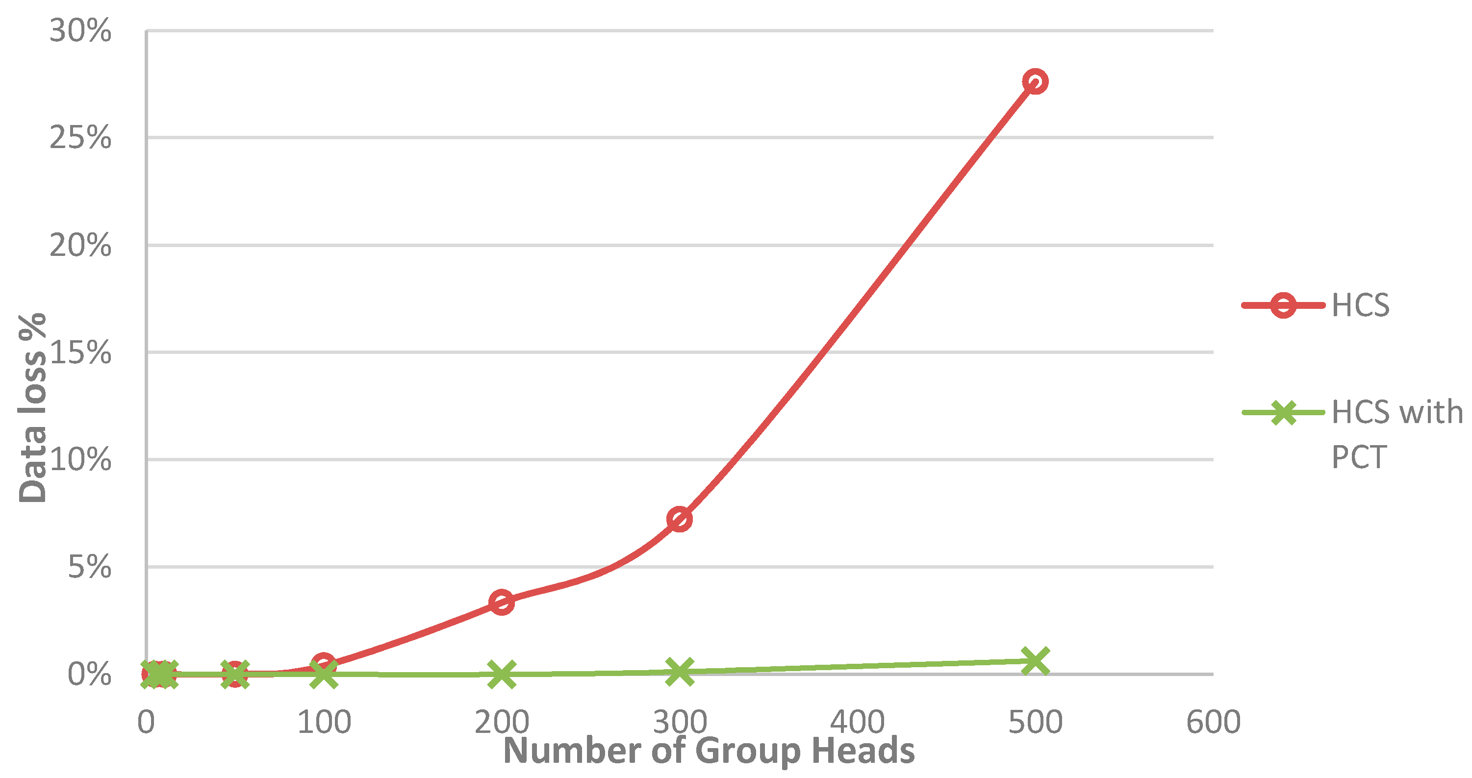
Therefore, HCS with PCT reduces the data collection path of MS since only those GHs that detect phenomena will participated in the reporting to MS. This reduces the consumed energy of network (see Figure 5) as compared to the HCS, in which all GHs participate in reporting to MS.
4.3.2. LUT
LUT reduces the energy cost by performing the election of new GHs (see Figure 1), and thus forming the groups, at the end of every nth window instead of at the end of every window. The selected n value will be fixed for all GHs across the mWSN. Note that LUT is applied on top of PCT. That is after computing data collection path of PCT the path will remain the same for fixed for n windows. By delaying the overhead of electing new GHs, LUT reduces the overall energy cost of mWSN as compared with HCS with PCT (without using LUT). However, the chances of losing some phenomena data becomes higher as the value of n increases. The reason is that as GHs are not updated across windows, the possibility of phenomena moving to other regions increases after the first window (n = 1).
5. Energy Cost Model
This section provides detailed analysis of the energy cost for the proposed algorithms. The two most critical sources of energy cost that impact the lifetime of the sensors and were the main focus of research in this field are the communication energy cost and the computation energy cost [23,31]. Another source of energy cost is the memory storage cost of the sensors [32]; however, due to the nature of our application, collected information by a mobile sensor within a window are discarded when the window ends. Communication cost is defined as the energy cost required for sending or receiving packets between two different sensors. The computation cost is defined as the energy cost required by the sensor’s CPU to perform computational operations.
Table 1 compares the communication cost with the computations cost of a sensor with processor MSP-430 and radio antenna CC2420, which are common characteristics in mWSNs. Table 2 shows that the wireless communication cost is three orders of magnitude more than the computational cost of the sensor. Therefore, the proposed algorithms focus on minimizing the communication cost. We assume a scheduling scheme such as ALOHA-Q [33,34], is used to minimize the energy cost during rebroadcasting information and idle listening; therefore, the resulting energy cost from idle listening is minimal and can be ignored. The amount of energy required to send j packets from one sensor to another . is computed as in [3,33].
where Etrans is the energy cost in the sensor’s transmitter electronics and Ereceive is the energy consumed by a sensor while receiving a k-bit packet. The parameter k is the packet size in bits, d is the distance between the sending and the receiving sensors, and α is the path loss exponent that expresses the radio frequency propagation path loss suffered over the wireless channel [35]. We assume that all sensors have the same sensing range and thus it is valid to assume that d is fixed for all sensors. Note that the communication cost depends greatly on the distance between the sender and the receiver sensors powered to α.
Below we discuss the energy cost of the different phases of the proposed phenomena detection algorithm.
I. Group Formation
The elected GHs for the current window broadcast their new status to inform other sensors in the network. Since a GH broadcast cannot reach the whole environment; therefore, we assume that each non-elected sensor rebroadcasts the announcement messages it receives from each elected GH once. The energy cost per sensor in this phase is as follows:
where the broadcast cost * NGH is the cost of rebroadcasting the messages of the NGH group heads, and ER(j, k)* NS * NGH is the cost of receiving the broadcasts of the NGH group heads. Hence, the total energy cost ξ1 for this phase by all sensors NS is
After GHs announce themselves as the new group heads, each sensor associates itself to the closest GH.
II. Local Phenomena Reporting
In this phase, each GHi gathers information from the sensors in its group and forms a local view of the phenomena. The sensors of each group report their information (speed, direction, location, remaining battery power) along with the phenomena information to their GHs. The sensor’s information is used in the GH election phase to determine the new GHs. Note that the proposed algorithms use the DGH election algorithm in [3] to elect the new GHs of the next window. Hence, the energy cost per GH and energy cost per member sensor in a group are given by Equations (5) and (6), respectively.
where represents the size of sensors’ information and represents the size of the detected phenomenon information if it exists. Thus, the total energy cost ξ2 for this phase is:
III. Data Collection by Mobile Sink
In this phase, as the mobile sink pass by a GH, the GH delivers its collected data collect to the mobile sink. The energy cost per GH is:
where d is the distance between the GH and the mobile sink, j is the number of packets that contain the data of every reporting sensor in the group, and NPM is the number of sensor that reported the local phenomena information in the group. The distance d is fixed between all GHs and the mobile sink. Therefore, the total energy cost ξ3 for this phase is:
IV. Group Heads Election for Next Window
In this phase, GHs are electeda for the next window using the DGH election algorithm proposed by [3]. The election of new GHs is purely computational performed by the current GHs with no required communication. Thus, the energy cost of this phase is negligible.
Therefore, the total energy cost ξtotal of all phases is:
6. Experimental Results
This section evaluates the time and energy consumption of the proposed phenomena detection algorithm, HCS, and the optimization algorithms. We implemented HCS as explained in Section 5. In the implementation of Phase four, we adopted the distributed group head election algorithm, called DGH, that was proposed by [3] to elect the new set of GHs for the following window. In DGH, at the end of every window wi, each group independently chooses its GH for the next time window wi+1. That is each current GH in wi selects the most suitable sensor in its group to be the next GH of the group. The selection criteria of new GH is based on the closeness of the sensor to existing phenomena (if any), in addition to the remaining battery power, speed, and direction.
The mWSN was implemented using the network simulator NS2. Table 3 presents the values of the different parameters used in the experiments. All experiments are performed on a PC running Ubuntu with Intel Core 2 Duo CPU 2.20 GHz, and 4 GB of RAM.
6.1. Evaluation of the Data Collection Strategy
Given an mWSN with fixed number of mobile sensors, the experiment in Figure 3 measures the effect of different orderings of GHs (different data collection paths) on the total time required to collect phenomena information for different number of groups. The experiment compares the proposed Hilbert-based ordering of GHs, which constitutes the data collection path of MS, with other orderings of the GHs, such as the Random, Z-order and Spiral. In Figure 3, the x-axis represents the number of GHs in the environment and the y-axis represents the total time required to collect the data from all GHs. The time values in this experiment are the average of 50 experiments.
Figure 3 shows that the Hilbert based ordering of GHs, which is used by the proposed HCS algorithm, requires the least time to collect data from all GHs. That is Hilbert ordering results in the shortest data collection path of MS. The Hilbert ordering achieves a saving of more than 90.0% of the total data collection time required by the Random approach, more than 88.0% as compared to the Spiral approach, and more than 25.0% as compared to the Z-order approach.
Figure 4 measures the effect of different orderings of GHs (different data collection paths of MS) on the data loss for different number of GHs. Note that the number of GHs is equivalent to the number of groups in the environment. Also, since the number of mobile sensors is fixed, the number of GHs gives an indication of the average size of the formed groups. The more GHs in the environment the smaller the average size of the groups and vice versa. In Figure 4 the x-axis represents the number of GHs in the environment and the y-axis represents the percentage of data loss. The values in the figure are the average of 50 experiments.
In this experiment, we fixed the window time, w, to be large enough to collect data from 100 GHs using Hilbert-based ordering. That is, the data collection time τ of MS in this experiment is equal to w. Thus, this window time is used to compute the percentage of data loss for all orderings of GHs (Hilbert, Z-order, Spiral and Random) across different number of GHs (see Figure 4). The data loss occurs when a new window wi+1 starts before the data of the current window wi is collected by MS. Note that for Hilbert-based ordering of GHs the percentage of data loss is zero when the number of GHs is less than, or equal to, 100; then, the percentage of data loss starts to increase gradually. It is shown that the percentage of data loss when using Hilbert ordering (proposed by HCS) is the lowest as compared with the other orderings of GHs. This result confirms that Hilbert-based ordering of GHs gives the shortest data collection path for MS as compared to other orderings of GHs. For example, with 200 GHs in the environment (about 20% of all GHs), a data loss of 3% for Hilbert-based ordering, 12% for Z-order, and 74% for both Random and Spiral ordering.
6.2. Evaluation of the Optimization Techniques
To further reduce the energy cost of the mWSN, we propose two data collection optimization techniques to the proposed HCS, namely the Phenomena-aware Collection Technique (PCT) and Lazy Update Technique (LUT). PCT shortens the data collection time and thus reduces data loss by limiting the number of GHs reporting the phenomena to MS. That is, the data collection path of MS is shortened to only include those GHs that detected local phenomena. On the other hand, LUT reduces the energy cost by performing the election of new GHs, and thus forming the groups (see Figure 6), at the end of every nth window instead of at the end of every window. By delaying the overhead of electing new GHs, and thus forming the groups, LUT reduces the overall energy cost of mWSN.
6.2.1. Effect of PCT
In Figure 5, given an mWSN with fixed number of mobile sensors, this experiment compares the percentage of data loss of the proposed HCS with that of the HCS with PCT. Note that HCS with PCT is similar to the HCS except that MS passes by only the GHs that detected the phenomena instead of all GHs in the environment. The experiment compares HCS and the HCS with PCT algorithms on the data loss for different number of GHs. In Figure 5, the x-axis represents the number of GHs in the environment and the y-axis represents the percentage of data loss averaged over 50 experiments. In this experiment, we fixed size of the phenomena and the number of GHs that detected the phenomena to 100 GHs. Figure 5 shows that percentage of data loss of HCS with PCT algorithm is much lower than that of HCT. This is due to the fact that in HCS with PCT only the GHs that detected the local phenomena report the phenomena to MS and thus the data collection path of MS is shorter than a path the includes all GHs in the environment. Therefore, MS is able to visit more GHs, which have data, and thus reduce the data loss. Note that the data loss results from the fact that a new window starts before MS can visit all GHs. The collected data at the unvisited GHs by MS will lost.
6.2.2. Effect of LUT
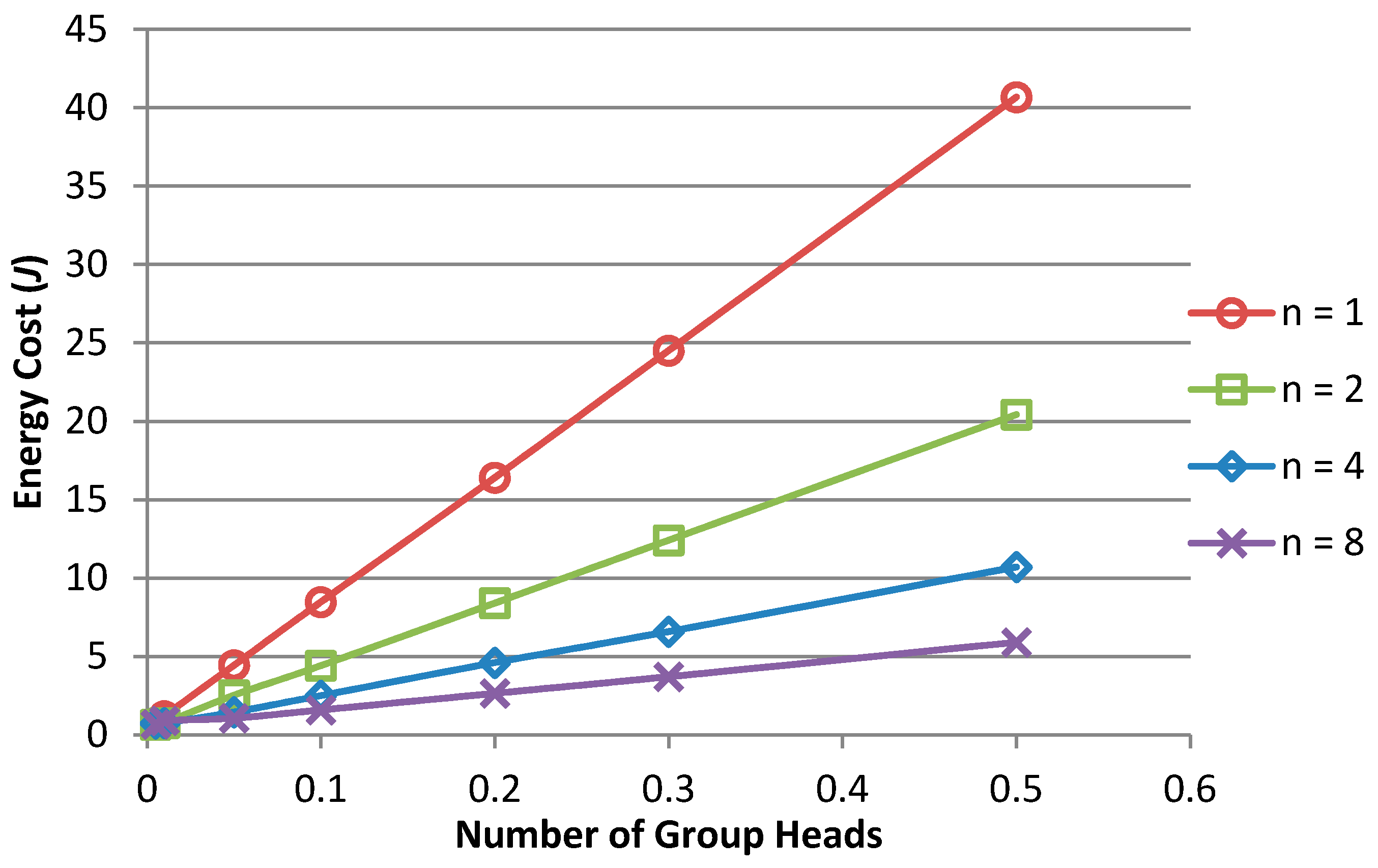
Given an mWSN with fixed number of mobile sensors, the experiment in Figure 6 compares the energy cost of the proposed HCS with the LUT. It measures the effect of the lazy update of new GHs on the total energy cost of the mWSN for different number of groups. In Figure 6, the x-axis represents the number of GHs in the environment and the y-axis represents the total energy cost averaged over 50 experiments. The experiment is conducted for updates at the end of the nth window, where n = 1, 2, 4 and 8.
Figure 7 shows that total energy cost by updating every 8th window is the lowest. HCS corresponds to the case where n = 1; that is the update of new GHs is performed at the end of every window. Therefore, the proposed LUT optimization reduces the energy cost as compared to HCS. However, the chances of losing some phenomena data becomes higher as the value of n increases. The reason is that as the frequency of updating the GHs becomes lower, the possibility of phenomena moving to other regions increases. As a result, in lazy update, some GHs that did not detect the phenomena in the first window (n = 1) might detect the phenomena in subsequent windows (n > 1), but their data will not be collected since the MS is not aware of them. In addition, other GHs that detected phenomena in the first window might not detected it in the following windows (n > 1) since the phenomena has drifted away.
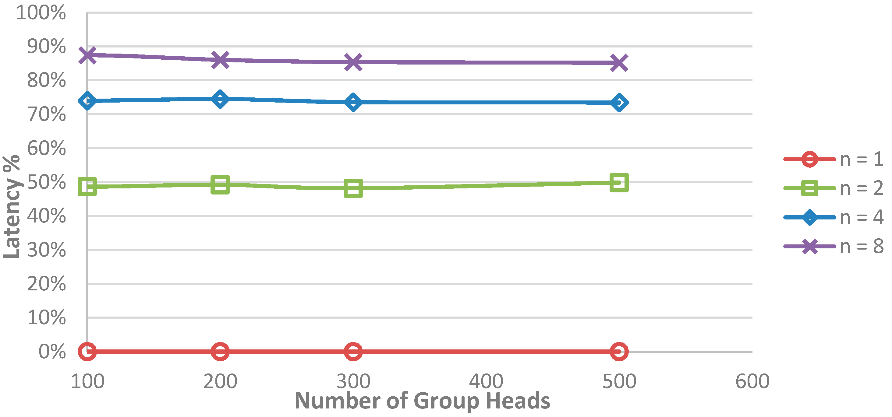
Figure 6 investigates the latency of data when using LUT, where the latency is defined as the waiting time of the collected data at the GHs until they are collected by MS. That can be measured by the percentage of GHs that detected the phenomena but MS is not aware of them and will not be visited until the GHs are updated at the end of the nth window. In this experiment, MS passes by only the GHs that detected phenomena at n = 1 and for the following windows (n > 1) MS keeps visiting the same set of GHs without updating it although a new set of GHs has already detected phenomena. Figure 6 measures the effect of lazy updates on latency for different number of GHs. The LUT is applied at the end of the nth window (n = 1, 2, 4 and 8) and latency is measured in terms of the percentage of unvisited GHs. In Figure 6, the x-axis represents the number of GHs in the environment and the y-axis represents the latency averaged over 50 experiments. HCS corresponds to the case where n = 1; that is the update of new GHs is performed at the end of every window. Figure 6 shows that the latency when n = 1 is the lowest (almost no latency) as compared with higher values of n. This is because when n = 1, the GHs will be updated every window and thus MS will have an updated list of GHs that detected phenomena. At n > 1, more and more GHs detect the phenomena but are not visited by MS causing more and more latency.
7. Conclusions
This paper addresses the problem of detecting phenomena such as oil spills, air pollution, etc., in the IoT environment. The environment consists of mobile sensors, mWSN and a mobile sink, MS. We proposed a distributed energy-efficient scheme to detect environmental phenomena from the data collected by the mWSN. These mobile sensors self-organize themselves into groups and elect a GH for each group. Each GH collects data from sensors in its group to detect possible local phenomena. The MS passes by GHs’ locations to collect the group’s data and discover the global phenomena. To reduce the energy cost of the mWSN, the paper proposes an efficient data collection strategy, called HCS. In HCS, the order of data collection by MS is based on the Hilbert-order of all GHs’ locations. To further reduce the energy cost of mWSN, the paper proposes two data collection optimization techniques.
The proposed solutions are validated using a comprehensive set of experiments. We implemented the mWSN using NS2 network simulator. Our simulation results show that HCS achieved a saving in the energy cost around 91.4% as compared to the base algorithm (Random). By combining HCS with PCT, the data loss decreased by 97.7% as compared with the HCS algorithm. Furthermore, LUT reduced the energy cost by about 50% if LUT is applied at n = 2 and 75% if it was applied at n = 4.
Author Contributions
Amany Abu Safia, Zaher Al Aghbari and Ibrahim Kamel are responsible for the concept of the paper, the mathematical soundness of the theory, design of experiments, data analytics aspects and the writing; Amany Abu Safia performed the experiments; all authors read and approved the paper.
Conflicts of Interest
The authors declare no conflict of interest.
References
- Zhang, D.; Yang, L.T.; Chen, M.; Zhao, S.; Guo, M.; Zhang, Y. Real-Time Locating Systems Using Active RFID for Internet of Things. IEEE Sens. J. 2016, 10, 1226–1235. [Google Scholar] [CrossRef]
- Al Aghbari, Z.; Kamel, I.; Elbaruni, W. Energy-efficient distributed wireless sensor network scheme for cluster detection. Int. J. Parallel Emerg. Distrib. Syst. 2012, 28, 1–28. [Google Scholar] [CrossRef]
- Safia, A.A.; Al Aghbari, Z.; Kamel, I. Phenomena Detection in Mobile Wireless Sensor Networks. Int. J. Netw. Syst. Manag. 2016, 24, 92–115. [Google Scholar]
- Doolin, D.M.; Sitar, N. Wireless sensors for wildfire monitoring. In Proceedings of the International Society for Optics and Photonicson Smart Structures and Materials, London, UK, 30–31 October 2005; pp. 477–484. [Google Scholar]
- Wichmann, A.; Korkmaz, T. Smooth path construction and adjustment for multiple mobile sinks in wireless sensor networks. Comput. Commun. 2015, 72, 93–106. [Google Scholar] [CrossRef]
- Rajesh, B.; Saravanan, K.A. An Improvised Effective Oceanography Monitoring Using Large Area Underwater Sensor Networks. In Geostatistical and Geospatial Approaches for the Characterization of Natural Resources in the Environment; Janardhana Raju, N., Ed.; Springer: New York, NY, USA, 2016; pp. 691–699. [Google Scholar]
- Bokareva, T.; Hu, W.; Kanhere, S.; Ristic, B.; Gordon, N.; Bessellet, T.; Rutten, M.; Jha, S. Wireless sensor networks for battlefield surveillance. In Proceedings of the Land Warfare Conference, Brisbane, Australia, 24–27 October 2006. [Google Scholar]
- Valverde, J.; Rosello, V.; Mujica, G.; Portilla, J.; Uriarte, A.; Riesgo, T. Wireless sensor network for environmental monitoring: Application in a coffee factory. Int. J. Distrib. Sens. Netw. 2012, 2012, 1–18. [Google Scholar] [CrossRef]
- Hao, X.; Jin, P.; Yue, L. Efficient Storage of Multi-Sensor Object- Tracking Data. IEEE Trans. Parallel Distrib. Syst. 2016, 27, 2881–2894. [Google Scholar] [CrossRef]
- Rao, J.; Biswas, S. Analyzing multi-hop routing feasibility for sensor data harvesting using mobile sinks. J. Parallel Distrib. Comput. 2012, 72, 764–777. [Google Scholar] [CrossRef]
- Zhang, Y.; Meratnia, N.; Havinga, P. Outlier detection techniques for wireless sensor networks: A survey. IEEE Commun. Surv. Tutor. 2010, 12, 159–170. [Google Scholar] [CrossRef]
- Rajasegarar, S.; Leckie, C.; Palaniswami, M.; Bezdek, J.C. Distributed anomaly detection in wireless sensor networks. In Proceedings of the IEEE Singapore International Conference on Communication Systems, Singapore, 30 October–2 November 2006; pp. 1–5. [Google Scholar]
- Kamel, I.; Al Aghbari, Z.; Awad, T. MG-join: Detecting phenomena and their correlation in high dimensional data streams. Distrib. Parallel Databases 2010, 28, 67–92. [Google Scholar] [CrossRef]
- Wittenburg, G.; Dziengel, N.; Wartenburger, C.; Schiller, J. A system for distributed event detection in wireless sensor networks. In Proceedings of the 9th ACM/IEEE International Conference on Information Processing in Sensor Networks, Stockholm, Sweden, 12–15 April 2010; pp. 94–104. [Google Scholar]
- Martincic, F.; Schwiebert, L. Distributed event detection in sensor networks. In Proceedings of the International Conference on Systems and Networks Communications, Tahiti, France, 29 October–3 November 2006; p. 43. [Google Scholar]
- Sheng, B.; Li, Q.; Mao, W.; Jin, W. Outlier detection in sensor networks. In Proceedings of the 8th ACM International Symposium on Mobile Ad Hoc Networking and Computing, Montreal, QC, Canada, 9–14 September 2007; pp. 219–228. [Google Scholar]
- Branch, J.W.; Giannella, C.; Szymanski, B.; Wolff, R.; Kargupta, H. In-network outlier detection in wireless sensor networks. Knowl. Inf. Syst. 2013, 34, 23–54. [Google Scholar] [CrossRef]
- Liu, C.M.; Lee, C.H.; Wang, L.C. Distributed clustering algorithms for data-gathering in wireless mobile sensor networks. Parallel Distrib. Comput. 2007, 67, 1187–1200. [Google Scholar] [CrossRef]
- Liu, C.M.; Lee, C.H. Power efficient communication protocols for data gathering on mobile sensor networks. In Proceedings of the 60th IEEE Vehicular Technology Conference, Los Angeles, CA, USA, 26–29 September 2004; pp. 4635–4639. [Google Scholar]
- Liu, C.M.; Lee, C.H.; Wang, L.C. Power-efficient communication algorithms for wireless mobile sensor networks. In Proceedings of the 1st ACM International Workshop on Performance Evaluation of Wireless Ad Hoc, Sensor, and Ubiquitous Networks, Venezia, Italy, 4–7 October 2004; pp. 121–122. [Google Scholar]
- Davies, V.A. Evaluating Mobility Models within an Ad Hoc Network. Ph.D. Thesis, Department of Mathematical and Computer Sciences, Colorado School of Mines, Golden, CO, USA, 2000. [Google Scholar]
- Royer, M.; Melliar-Smith, P.M.; Moser, L.E. An analysis of the optimum node density for ad hoc mobile networks. In Proceedings of the IEEE International Conference on Communications, Helsinki, Finland, 11–14 June 2001; Volume 3, pp. 857–861. [Google Scholar]
- Zhao, H.; Guo, S.; Wang, X.; Wang, F. Energy-efficient topology control algorithm for maximizing network lifetime in wireless sensor networks with mobile sink. Appl. Soft Comput. 2015, 34, 539–550. [Google Scholar] [CrossRef]
- Tunca, C.; Isik, S.; Donmez, M.Y.; Ersoy, C. Ring routing: An energy-efficient routing protocol for wireless sensor networks with a mobile sink. IEEE Trans. Mob. Comput. 2015, 14, 1947–1960. [Google Scholar] [CrossRef]
- Zhu, C.; Han, G.; Zhang, H. A honeycomb structure based data gathering scheme with a mobile sink for wireless sensor networks. Peer-to-Peer Netw. Appl. 2017, 10, 484–499. [Google Scholar] [CrossRef]
- Wang, W.; Shi, H.; Wu, D.; Huang, P.; Gao, B.; Wu, F.; Xu, D.; Chen, X. VD-PSO: An efficient mobile sink routing algorithm in wireless sensor networks. Peer-to-Peer Netw. Appl. 2017, 10, 537–546. [Google Scholar] [CrossRef]
- Tang, X.; Xie, L. Data Collection Strategy in Low Duty Cycle Wireless Sensor Networks with Mobile Sink. Int. J. Commun. Netw. Syst. Sci. 2017, 10, 227–239. [Google Scholar] [CrossRef]
- Chen, Y.; Lv, X.; Lu, S.; Ren, T. A Lifetime Optimization Algorithm Limited by Data Transmission Delay and Hops for Mobile Sink-Based Wireless Sensor Networks. J. Sens. 2017, 2017, 7507625. [Google Scholar] [CrossRef]
- Nayak, S.P.; Rai, S.C.; Pradhan, S. A Multi-clustering Approach to Achieve Energy Efficiency Using Mobile Sink in WSN. In Proceedings of the 3rd International Conference on Computational Intelligence in Data Mining, Singapore, 10–11 December 2016; pp. 793–801. [Google Scholar]
- Shekhar, S.; Chawla, S. Spatial Databases: A Tour; Prentice Hall: Upper Saddle River, NJ, USA, 2003. [Google Scholar]
- Shi, L.; Johansson, K.H.; Murray, M. Estimation over wireless sensor networks: Tradeoff between communication, computation and estimation qualities. In Proceedings of the 17th IFAC World Congress, Seoul, Korea, 6–11 July 2008; pp. 605–611. [Google Scholar]
- Mathur, G.; Desnoyers, P.; Chukiu, P.; Ganesan, D.; Shenoy, P. Ultra-low power data storage for sensor networks. ACM Trans. Sens. Netw. 2009, 5, 1–34. [Google Scholar] [CrossRef]
- Chu, Y.; Kosunalp, S.; Mitchell, P.D.; Grace, D.; Clarke, T. Application of reinforcement learning to medium access control for wireless sensor networks. Eng. Appl. Artif. Intell. 2015, 46, 23–32. [Google Scholar] [CrossRef]
- Chu, Y.; Mitchell, P.D.; Grace, D.; Clarke, T. Use of Q-learning approaches for practical medium access control in wireless sensor networks. Eng. Appl. Artif. Intell. 2016, 55, 146–154. [Google Scholar]
- Dimitriou, G.; Kikiras, P.K.; Stamoulis, G.I.; Avaritsiotis, I.N. A tool for calculating energy consumption in wireless sensor networks. In Proceedings of the 10th Panhellenic Conference on Informatics, Volos, Greece, 11–13 November 2005; pp. 611–621. [Google Scholar]
Figure 1.
Phases of phenomena detection in the proposed scheme.

Figure 2.
An example that shows the data collection path of all group heads.

Figure 3.
Comparing the total time required of by the mobile sink to collect data from all group heads (GHs) using different orderings of GHs (different collection paths).
Figure 3.
Comparing the total time required of by the mobile sink to collect data from all group heads (GHs) using different orderings of GHs (different collection paths).

Figure 4.
Comparing the percentage of data loss using different orderings of GHs.
Figure 5.
Comparing the data loss percentage using Hilbert Collection Strategy and different participating strategy.
Figure 5.
Comparing the data loss percentage using Hilbert Collection Strategy and different participating strategy.

Figure 6.
Average latency cost of detecting phenomena when using Lazy Update Technique (LUT).

Figure 7.
Effect of LUT at the end of the nth window (n = 1, 2, 4 and 8).


Table 1.
Definitions of the frequently used symbols.
| Symbol | Definition |
|---|---|
| GH | Sensor elected as a group head |
| NS | The number of mobile sensors |
| MS | The mobile sink |
| τ | the trip time (see Definition 2) |
| w | Window time (see Definition 1) |
| NGH | The number of elected group heads |
| NGM | The number of sensors in a group |
| NPM | The number of sensors which detected phenomena inside a group |
| ET | Energy cost by the sensor’s transmitter |
| ER | Energy cost by the sensor’s receiver |
Table 2.
The computation cost and communication cost per byte data.
| MSP-430 Instruction Computation | CC2420 Radio Transmission | CC2420 Radio Receiving | |
|---|---|---|---|
| Energy (μJ/byte) | 0.0008 | 1.8 | 2.1 |
| Ratio | 1 | 2250 | 2600 |
Table 3.
Parameter values used in the experiments
| Variable | Value |
|---|---|
| ET | 1.8 μJ/byte |
| ER | 2.1 μJ/byte |
| NS | 1000 mobile sensors |
| NGH | 5, 10, 50, 100, 200, 300, 500 |
| K | 5 bytes |
| Sensor Speed | Range 0–5 m/s |
| α | 2 |
© 2017 by the authors. Licensee MDPI, Basel, Switzerland. This article is an open access article distributed under the terms and conditions of the Creative Commons Attribution (CC BY) license (http://creativecommons.org/licenses/by/4.0/).
Share and Cite
MDPI and ACS Style
Safia, A.A.; Aghbari, Z.A.; Kamel, I. Efficient Data Collection by Mobile Sink to Detect Phenomena in Internet of Things. Information 2017, 8, 123. https://doi.org/10.3390/info8040123
AMA Style
Safia AA, Aghbari ZA, Kamel I. Efficient Data Collection by Mobile Sink to Detect Phenomena in Internet of Things. Information. 2017; 8(4):123. https://doi.org/10.3390/info8040123
Chicago/Turabian StyleSafia, Amany Abu, Zaher Al Aghbari, and Ibrahim Kamel. 2017. "Efficient Data Collection by Mobile Sink to Detect Phenomena in Internet of Things" Information 8, no. 4: 123. https://doi.org/10.3390/info8040123
Note that from the first issue of 2016, this journal uses article numbers instead of page numbers. See further details here.