The Current Role of Image Compression Standards in Medical Imaging
by
 ,
,
Feng Liu
1 ,
,
Miguel Hernandez-Cabronero
2,
Victor Sanchez
3,
Michael W. Marcellin
2 and
Ali Bilgin
2,4,5,* 1
College of Electronic Information and Optical Engineering, Nankai University, Haihe Education Park, 38 Tongyan Road, Jinnan District, Tianjin 300350, China
2
Department of Electrical and Computer Engineering, The University of Arizona, 1230 E. Speedway Blvd, Tucson, AZ 85721, USA
3
Department of Computer Science, University of Warwick, Coventry CV4 7AL, UK
4
Department of Biomedical Engineering, The University of Arizona, 1127 E. James E. Rogers Way, Tucson, AZ 85721, USA
5
Department of Medical Imaging, The University of Arizona, 1501 N. Campbell Ave., Tucson, AZ 85724, USA
*
Author to whom correspondence should be addressed.
Information 2017, 8(4), 131; https://doi.org/10.3390/info8040131
Submission received: 25 September 2017
/
Revised: 13 October 2017
/
Accepted: 15 October 2017
/
Published: 19 October 2017
(This article belongs to the Section Review)
Abstract
:With the increasing utilization of medical imaging in clinical practice and the growing dimensions of data volumes generated by various medical imaging modalities, the distribution, storage, and management of digital medical image data sets requires data compression. Over the past few decades, several image compression standards have been proposed by international standardization organizations. This paper discusses the current status of these image compression standards in medical imaging applications together with some of the legal and regulatory issues surrounding the use of compression in medical settings.
Keywords:
image compression; medical imaging; standards; JPEG; JPEG-LS; JPEG2000; JPEG-XR; HEVC; DICOM1. Introduction
Medical imaging has become an indispensable tool in clinical practice. Studies have shown links between the use of medical imaging exams and declines in mortality, reduced need for exploratory surgery, fewer hospital admissions, shorter hospital stays, and longer life expectancy [1]. As a result, the utilization of medical imaging has risen sharply during the early part of the last decade. In 2003, the percentage of medical visits in the US by patients aged years that resulted in medical imaging was estimated to be 12.8% [2]. While earlier medical imaging exams were recorded on radiological film, most exams are now acquired digitally. In addition to increased utilization, there have also been major advances in medical imaging technology that have resulted in significant increases in the quantity of digital medical imaging data during the last few decades. For example, in early 1990s, a typical Computed Tomography (CT) exam of the thorax would have consisted of 25 slices with 10 mm thickness, yielding a data size of roughly 12 megabytes (MBs). Today, a similar exam on a modern CT scanner can yield sub-millimeter slice thickness with increased in-plane resolution resulting in 600 MB to a gigabyte (GB) of data. In a modern hospital, Picture Archiving and Communication Systems (PACS) handle the short- and long-term storage, retrieval, management, distribution, processing, and presentation of these large datasets. Data compression plays an important role in these systems. Since the earliest days of PACS, compression of medical images has been anticipated and novel compression techniques have been proposed before standardized compression approaches were available [3]. However, proprietary compression techniques greatly increase the cost and effort required to migrate data between different systems, and interoperability and compatibility of these systems necessitate the use of standards for digital communications [4]. In this paper, we provide a review of the current status of image compression standards used for medical imaging data in these systems (It is also worthwhile to point out that the role of data compression in the medical setting is not limited to images. Modern medical practice utilizes many physiological signals (e.g., electrocardiogram (ECG), electroencephalogram (EEG), and Electromyogram (EMG)) which must be stored and transmitted in clinical practice. Data compression has an important role to play for management of such physiological signals as well. However, in this paper, we limit our discussion to medical images). It is important to note that there have been earlier reviews of medical image compression techniques [5,6,7,8,9,10,11,12,13,14]. In this paper, we focus on the image compression standards including the more recent standards that have not been considered in these earlier reviews. We also compare the compression performances of these standards on publicly available datasets.
The rest of this paper is organized as follows: In Section 2, we discuss characteristics of common medical imaging data sets. In Section 3, we provide a brief introduction to current image compression standards. Section 4 introduces the standards used for medical image communications. Section 5 briefly reviews the current legal and regulatory environment in medical image communications. We present experimental results obtained using the image compression standards on typical medical image datasets in Section 6. Finally, Section 7 provides a summary and a brief discussion on future trends.
2. Characteristics of Medical Imaging Data Sets
The purpose of this section is to briefly describe the unique attributes of the major medical imaging modalities. Medical imaging refers to techniques used to view the human body with the goal of diagnosing, monitoring, and/or treating medical conditions. Different imaging modalities are based on different physical principles and provide different information about structure, morphology, and function of the human body. Medical imaging is an active field with new imaging modalities introduced frequently and existing modalities refined and expanded constantly. Given this depth and diversity of the medical imaging field, it is not realistic to provide a complete description of all medical imaging techniques in this section. Therefore, we limit our discussion to the most common medical imaging methods in clinical practice and their general characteristics as they relate to data compression (For an extended review of the characteristics of medical datasets, the interested reader is referred to [15]). Table 1 provides the typical image dimensions and uncompressed file sizes for common medical imaging modalities.
2.1. Digital Radiography and Computed Tomography
In X-ray radiography, the subject is penetrated by a collimated beam of X-rays and the properties of the X-ray (intensity, energy spectrum, direction of propagation, etc.) are modified as it travels through the human body. An array of X-ray detectors placed behind the subject is then used to record the modified properties of the X-ray beam and form the X-ray image. The dimensions of the image depend on the dimensions of the detector elements (0.1 mm to 0.2 mm) and the field of view ( cm to cm based on the anatomy of interest). A sample X-ray image of the pelvis is shown in Figure 1a.
In X-ray radiography, a single projection plane of an anatomical region is imaged onto the detector plane. In contrast, CT imaging produces a 3D image of the anatomy of interest by acquiring several projections at different angles and reconstructing the 3D volume using tomography [16]. Today’s multi-detector row CT scanners can acquire up to 320 simultaneous slices in each rotation of the X-ray tube. A thin-slice CT dataset can contain over 500 slices and dynamic imaging (such as cardiac angiography or perfusion imaging) can be performed on the latest generation of CT scanners although the routine clinical utilization of these studies is limited due to concerns about radiation dose. Another recent X-ray imaging technique developed to enhance characterization of breast lesions is Digital Breast Tomosynthesis (3D Mammography) [17,18]. In this technique, thin sections of the breast tissue are reconstructed through acquisition of multiple projections over a limited arc angle. These use of thin slices covering the entire breast allows better visualization and characterization of masses that may otherwise be superimposed with out-of-plane structures.
A sample CT image of an axial slice of the abdomen is shown in Figure 1b. The contrast resolution in CT is largely determined by the number of photons per voxel and, therefore, there is a trade-off between X-ray dose and contrast resolution, as well as spatial resolution. Noise in CT images originates from a number of sources including photon noise at the detector, electronic noise of the detector system, and the image reconstruction algorithm used.
2.2. Magnetic Resonance Imaging
Magnetic Resonance Imaging (MRI) [19] is based on the principles of nuclear magnetic resonance. In MRI, the contrast of the image is dependent on several tissue-dependent parameters as well as the choice of acquisition parameters selected during the imaging procedure. By varying these parameters, MRI can yield images with drastically different contrast. This is illustrated in Figure 2 where an axial slice of the brain was imaged using different imaging parameters. This ability to obtain different image contrasts by selecting different imaging parameters is what gives MRI its tremendous flexibility and has contributed to its significant clinical utility. MRI can differentiate between different soft tissue types such as white matter and grey matter in the brain and tumors and cysts in the liver. Furthermore, since MRI does not use the damaging ionizing radiation of X-rays, it is often favored in preference to CT in dynamic imaging applications where the radiation dose required to obtain the dynamic data set with CT would be prohibitive.
During a typical clinical MRI examination, multiple images of the same anatomy are obtained with different imaging parameters. The number of different contrasts acquired during a particular exam depends on the clinical application and is typically in the five to ten range. Thus, although the MRI images are usually obtained at lower spatial resolution compared to CT datasets, the number of different contrasts acquired during a typical exam results in substantial increase of data size.
The noise in MRI is mainly due to the thermal noise of the receiver coil and the sample, and can be modeled using Rician distributions [20].
2.3. Ultrasound
Ultrasound imaging is based on the principles of acoustics [21]. A sound wave is transmitted from a transducer which is placed directly on the skin or inside a body opening. The sound wave is partially absorbed and partially reflected as it travels through the tissue. The time of arrival of the echo and the intensity of the reflected wave are used to reconstruct an image of the tissue under examination.
In ultrasound, the spatial resolution is described in terms of axial resolution (i.e., the ability to resolve two reflectors located one after the other along the axis of the ultrasound wave) and lateral resolution (i.e., the ability to resolve two reflectors located side by side perpendicular to the axis of the ultrasound wave). Higher ultrasound beam frequencies lead to better axial and lateral resolution. However, since higher frequencies also lead to higher attenuation, there is often a trade-off between tissue depth and spatial resolution.
As a result of its relatively low-cost and safety due to the absence of ionizing radiation, ultrasound imaging is widely used in many clinical applications including obstetrics, cardiology, and cancer imaging in the abdomen and pelvis. Depending on the application, ultrasound data are acquired and viewed in many different modes: In A-mode (amplitude mode), the amplitudes of the echoes are plotted as a function of depth along a fixed direction. In B-mode (brightness mode), an array of transducers are used to create a 2D image where each pixel intensity denotes the amplitude of the echoes at a particular direction and depth. In M-mode (motion mode), a rapid succession of pulses is used to generate time-varying (typically B-mode) images. Ultrasound imaging is a rapidly advancing field. In addition to conventional ultrasound imaging techniques, many new expansions have been introduced over the last few decades. In 3D ultrasound, 2D planar ultrasound images are digitally stitched together to create a 3D image. Doppler ultrasound employs the Doppler effect to measure whether the tissue is moving towards or away from the transducer as well as its relative velocity.
The dominant noise in conventional B-mode ultrasound images is speckle noise which is signal-dependent and multiplicative in nature [22].
2.4. Nuclear Imaging
In nuclear imaging, small amounts of radioactive materials (radiopharmaceuticals) attached to compounds used by cells are given to the subject through an injection or orally. The radioactive substances are traced through imaging to determine where and when they concentrate in the body. Two common nuclear imaging modalities are Single Photon Emission Computed Tomography (SPECT) and Positron Emission Tomography (PET) [23]. In SPECT, gamma-rays emitted from a radioisotope are measured using a gamma-ray camera, while PET uses molecules tagged with a positron emitting isotope.
Clinical PET and SPECT scanners are often combined with other imaging modalities that can provide anatomical information so that functional and anatomical information can be acquired in one examination. PET-CT and PET-MRI systems are widely used in clinical settings.
The spatial resolution in SPECT is often limited (to about 1 cm). Therefore, the amount of data produced in SPECT imaging is modest compared to some of the other common medical imaging modalities. Similarly, the spatial resolution in PET is typically between 3 to 5 mm and, thus, PET data sets are relatively small as well. Noise in SPECT and PET systems are due to several factors including the Poisson distributed noise during emission, electronic noise in the scanner’s detection system, and the noise alterations due to the post-processing corrections and the image reconstruction process [24].
2.5. Digital Pathology
In digital pathology, thin slices of biological tissue are scanned using optical microscopy to produce the so-called whole-slide images [25]. Tissue samples are dyed using one or more stains to highlight the biological structures relevant to the diagnostic task, and then placed on a glass slide. Typically, a combination of hematoxylin and eosin (H&E) stains is employed to give nuclei and cytoplasm blue/purple and red/pink hues, respectively. A pathology image depicting H&E stained tissue is shown in Figure 3.
In the slide scanner, the sample is illuminated with a beam of visible white light, which is absorbed and scattered differently depending on the stain type and concentration present at each spatial location. Imaging optics are used to transmit an image of the patch of tissue under the microscope objective to a digital image sensor. The objective is moved back and forth across the glass slide to generate image patches that are then combined to produce the whole-slide image. For most tissue types and diagnostic tasks, optical magnifications of 20× are considered sufficient to identify the relevant biological features. Notwithstanding, higher magnifications of up to 100× may be required for some sample types, e.g., in cytopathology and hemathology.
As a result of the high spatial resolution employed in digital pathology, whole-slide images exhibit very large dimensions, commonly exceeding 900 million pixels. Moreover, since color is an essential feature for differentiating the different biological structures, each pixel consists of three color components. Thus, the size of a single uncompressed whole-slide image is usually over 2.5 GB. Since digital pathology requires digital storage, transmission, and, importantly, visualization of these large images, efficient organization of the compressed data for display of the image at different zoom levels and at different spatial regions is vital. Therefore, compressed-data reorganization capabilities (e.g., tiling in BigTIFF [26], tiled Digital Imaging and Communications in Medicine (DICOM) [27], or interactive multi-resolution transmission with JPIP [28]) are paramount to enable a smooth visualization experience.
3. Image Compression Standards
The advent and growth of digital imaging during the latter part of the last century have resulted in growing demand to transmit and store images digitally. Recognizing the need for compatibility and interoperability between different image communications and storage products, international standardization agencies, such as International Standards Organization (ISO), International Telecommunications Union (ITU), and International Electro-technical Commission (IEC), have initiated several standardization efforts for image compression over the past few decades. These standards have played a major role in fostering the growth of digital imaging. In this section, we provide a brief overview of these image compression standards.
3.1. JPEG
JPEG stands for “Joint Photographic Experts Group” and refers to the working group WG1 of the ISO/IEC Joint Technical Committee 1, Study Committee 29 (ISO/IEC JTC1/SC29/WG1). Over the past few decades, the WG1 committee has created several international standards for image compression. Standardization efforts start by formation of a technical committee (such as the WG1) and solicitation of proposals from interested parties including industry and academia. The technical committee prepares a working draft which is shared by all ISO national members. Once consensus is reached on the working draft, a final draft is created. The final draft becomes an international standard after it is approved by national member votes.
The WG1 committee started its work in the mid-1980’s. The first international standard produced by the committee is called JPEG, referring to the name of the committee that created it. The JPEG standard was released in 1991 [29,30] and has become one of the most widely recognized and utilized standards.
The JPEG standard consists of six parts: Part 1 describes the requirements and guidelines for JPEG compression systems [29]. Part 2 contains compliance testing [31]. Part 3 provides extensions to the compression system [32], and Part 4 discusses profiling and registration of profiles [33]. Part 5 specifies the JPEG File Interchange Format (JFIF) [34]. Finally, Part 6 contains application tools for printing systems [35].
Although the JPEG standard has several lossy encoding modes and a lossless encoding mode, many implementations support only a basic lossy coding algorithm with a minimal set of features. This algorithm is usually referred to as the “baseline JPEG” algorithm. The baseline JPEG encoder, shown in Figure 4, first partitions the image into non-overlapping blocks. Each block is then transformed using the two-dimensional Discrete Cosine Transform (DCT). In the DCT domain, the coefficient that corresponds to zero frequency is referred to as the DC coefficient of the block and all remaining coefficients are called AC coefficients. Each DCT coefficient is then quantized using a uniform scalar quantizer. The quantization step size varies with frequency and the array denoting the step size used for each frequency is known as the “Q-table”. The entries of the Q-table are stored in the bit-stream. The redundancy between DC coefficients of adjacent blocks is exploited using a simple differential pulse-code modulation (DPCM) encoding scheme followed by variable-length encoding and Huffman coding. The AC coefficients are zig-zag scanned. Since many AC coefficients become zero after quantization, they can be encoded efficiently using run-length coding followed by variable length coding.
The baseline algorithm discussed above is an instance of the JPEG sequential mode. Besides the baseline, the JPEG standard defines several options that can be utilized. For example, baseline JPEG restricts the input image bit depth to 8. Since most medical imaging modalities use bit depths between 10 and 16, this restriction would normally render JPEG unsuitable for compression of medical images. Fortunately, the JPEG standard provides options to support up to 12-bit imagery, which is suitable for certain types of medical images (e.g., ultrasound, CT, digital pathology) but not others (e.g., some MRI). Furthermore, in addition to the sequential mode, three additional modes of operation are defined. These are the progressive, the hierarchical, and the lossless modes. The latter employs DPCM followed by Huffman entropy coding and supports bit depths up to 16 bits. Despite its limited compression performance, this JPEG mode is the most widely used lossless compression scheme in medical applications today.
A software implementation of the JPEG standard was released by the Independent JPEG Group in 1991 [36] and has been continuously maintained since.
3.2. JPEG2000
In the late 1990s, the WG1 committee started an standardization process with the goal of improving upon the very successful JPEG compression standard. The desired features included enhanced bit-rate performance (specially at low bit-rates), support for samples of up to 16 bits deep, progressive transmission and lossless and lossy compression from a single architecture. Random access, error robustness and allowing for low-memory implementations were also required. As a result of this effort, JPEG2000 became a ISO/IEC Standard and ITU-T Recommendation in December 2000 [37]. Part 1 of this standard describes the core coding system, including the JPEG2000 codestream syntax and a basic file format called JP2. Part 2, published in November 2001, defines additional extensions to the core system. Several other parts were defined as well, including Part 9, which describes JPIP, a protocol for the interactive transmission of images [28], and Part 10 which describes JP3D for volumetric imaging [38].
The main stages of the JPEG2000 compression pipeline [39] are depicted in Figure 5. The spectral redundancy between the image components (e.g., color channels, spectral bands or time frames) can be removed in the multi-component transform (MCT) stage, transforming each pixel independently. In Part 1 of the standard, component decorrelation can be performed using a reversible or an irreversible color transform, which decorrelate RGB images to luminance and chrominance components. In Part 2, any number of components can be decorrelated using arbitrary MCTs, in some cases producing improvements in compression performance [40,41,42,43] (It is important to distinguish the Parts 2 and 10 of the JPEG2000 standard: Part 2 provides an MCT stage which can be used with volumetric data sets whereas Part 10 defines a 3D extension of the standard for volumetric imaging applications. As will be discussed in Section 4, the Part 2 has its own DICOM transfer syntax [44]; However, Part 10 has not been added to DICOM). In the second stage, the spatial decorrelation of each component is removed independently via a 2D discrete wavelet transform (DWT). In the first decomposition level of the DWT, the image is divided into the LL, HL, LH, and HH subbands, each of size . The three latter subbands contain high-frequency details, while the LL subband is a downscaled version of the original image. This decomposition is usually repeated five times using the LL subband of one iteration as the input for the next one. In addition to dealing with spatial correlation, the DWT provides an efficient multi-scale representation of the image. In the lossy coding regime, the DWT coefficients undergo a uniform dead-zone quantization, where values v such that are assigned to the same quantization interval as 0. In the lossless compression mode, the transformed coefficients are integers and are not quantized. In either mode, the resulting coefficients are divided into blocks of size by default. Each block is coded independently using an adaptive arithmetic coder called MQ. In the last stage, the compressed blocks are organized so that the final bit-stream can be progressively transmitted providing resolution, spatial, quality or component scalability. Region-of-interest coding, e.g., assigning higher priority to some spatial regions in the coding process, is also supported by JPEG2000 [45].
3.3. JPEG-LS
The JPEG-LS standard defines lossless and near-lossless compression methods for compressing bi-level, gray-scale, and color images [51]. JPEG-LS is based on the HP LOCO [52,53] codec, and its low complexity has played an important role in its selection for the Mars Spirit Rover project [54]. The standard is published in two parts: Part 1 of the standard defines the baseline algorithm [51] and Part 2 introduces extensions [55]. Baseline JPEG-LS scans the image pixels in raster-scan order and encodes each pixel using either the run mode or regular mode. The mode decision is made using a template of four neighboring pixels as illustrated in Figure 6. In the figure, X denotes the current pixel and A, B, C, and, D denote the neighboring pixels. Using these neighboring pixels, three difference values are formed:
The mode decision is made as follows:
During run mode, pixel values are coded using run-length coding. The run mode is terminated when a pixel is encountered that does not satisfy the above constraints, or when the end of a row is reached. For lossless coding, the value of is set to zero. For near-lossless coding, is set as a small integer indicating the maximum allowable deviation of pixel values from the original values.
In regular mode, a prediction of the current pixel value is formed using the following equation:
The prediction error is then coded using context modeling designed to exploit the high-order structural dependencies between pixel values.. Contexts are formed by quantizing the differences , , and into 9 values each. Assuming that the prediction error distribution is symmetric about the origin, the number of contexts is further reduced to . Conventional context modeling methods would use these contexts as conditioning states and adaptively estimate conditional probability models for the prediction errors for each context state during coding. Employing such methods with a large number of contexts would lead to context dilution. However, the JPEG-LS standard avoids this problem by estimating the conditional mean for each context. These estimates are then used in a procedure called bias cancellation to further refine the predictions. The bias-canceled prediction errors are encoded using Golomb codes [56].
JPEG-LS offers significant advantages in terms of its simple and easy to implement procedures, low memory footprint, and low computational complexity. Despite the simplicity of the coding procedures, the compression performance achieved by JPEG-LS is very competitive with methods that rely on more computationally demanding coding techniques such as arithmetic coding. Since JPEG-LS offers state-of-the-art lossless compression performance, it is particularly well suited for certain medical applications that demand lossless compression.
3.4. JPEG-XR
The JPEG-XR standard was developed with the primary goal of compressing continuous-tone still images such as photographic images [62]. The standard originated from the HD Photo technology developed by the Microsoft Corporation in 2007 [63] and was published in five parts: Part 1 of the standard [62] defines the system architecture and Part 2 [64] provides the image coding specifications. Parts 3 through 5 provide the Motion JPEG XR specification [65], conformance testing [66], and the reference software [67], respectively.
JPEG-XR was designed to provide high compression efficiency while also enabling low-complexity encoding and decoding implementations. Similar to JPEG, JPEG-XR is also a “block-transform” based image compression method. However, unlike JPEG which uses the DCT, JPEG-XR uses a hierarchical two-stage lapped biorthogonal transform (LBT) implemented using lifting steps. The LBT reduces the block-boundary artifacts which are commonly seen in JPEG-compressed images at high compression ratios. The resulting transform bands are compressed independently, allowing a multi-resolution hierarchy of up to 3 levels. The quantization stage of JPEG-XR offers flexible quantization step size selection. The quantization step size can be varied spatially, across frequency bands, and across color channels. The quantization step is followed by the inter-block coefficient prediction stage which aims to remove the dependencies between the quantized transform coefficients across blocks. JPEG-XR partitions the high-frequency data into two for layered coding: The so-called significant information is entropy coded and the remainder, which is considered to be incompressible, is signaled using fixed-length codes. JPEG-XR uses adaptive Variable Length Coding (VLC) tables which allows the best table to be chosen for entropy coding based on the statistics of local coefficients.
JPEG-XR has two key features that are important for medical image compression applications: First, JPEG-XR supports bit depths of up to 32 bits for the input image. Second, JPEG-XR supports both lossy and lossless compression using the same signal flow path.
3.5. H.265
The H.265 video coding standard, also known as the High Efficiency Video Coding (HEVC) standard, is proposed by the Joint Collaborative Team on Video Coding (JCT-VC), which is jointly established by the ITU-T Video Coding Experts Group (VCEG) and the ISO/IEC Moving Picture Expert Group (MPEG) [68]. HEVC/H.265 has been shown to attain significant improvements in coding efficiency for camera-captured material compared to earlier video coding standards, in the range of 50% bit-rate reduction for equal perceptual quality [68].
HEVC/H.265 follows the same general coding approach as its immediate predecessor standard, H.264/AVC [69]. Namely, each frame in a video sequence is first split into non-overlapping block-shaped regions. Each block is then predicted by using spatial data prediction within the same picture or by using data from previously coded frames through motion compensation and estimation. The former is referred to as intra-prediction, while the latter is referred to as inter-prediction. In both types of prediction, the main goal is to reduce the amount of data needed to represent each block at the best quality possible. HEVC/H.265 uses a quadtree-based coding structure with blocks ranging from 4 × 4 to 64 × 64 pixels. The residual signal, which is the difference between the original block and its prediction, is transformed using the two-dimensional DCT or Discrete Sine Transform (DST). The resulting transform coefficients are then scaled, quantized, entropy coded, and transmitted together with the prediction information. Context adaptive binary arithmetic coding (CABAC) is used for entropy coding in HEVC/H.265. This is similar to the CABAC in H.264/AVC, but with improvements to its throughput speed, compression performance, and context memory requirements. HEVC/H.265 includes a lossless coding mode that allows mathematically lossless reconstruction of a signal [70,71,72,73,74,75,76,77,78,79,80,81]. This is achieved by bypassing the transform, quantization, and other processing (sample adaptive offset and deblocking filters) that affects the decoded picture, and feeding the residual signal from inter or intra prediction directly into the entropy coder. Therefore, no additional coding tools are employed for lossless coding. Figure 7 depicts a simplified block diagram of an encoder capable of generating a compressed bit-stream compliant with the HEVC/H.265 standard [68].
The most important elements in the HEVC/H.265 intra-prediction process include [68]:
- 35 prediction modes, with 33 angular modes, one DC and one planar mode;
- adaptive smoothing of the reference samples; and
- filtering of the prediction block boundary samples.
The most important elements in the HEVC/H.265 inter-prediction process include [68]:
- improved motion compensation with quarter-sample precision for motion vectors (MVs), and 7-tap or 8-tap filters for interpolation of fractional sample positions;
- multiple reference pictures that allows transmitting one or two MVs for each block, resulting in unipredictive or bipredictive coding, respectively;
- advanced motion vector prediction, which includes derivation of several most probable candidate MVs based on data from adjacent blocks and the reference frame; and
- sample adaptive offset (SAO), which is a nonlinear amplitude mapping used after the deblocking filter with the objective to better reconstruct the original signal amplitudes.
HEVC/H.265 introduces data structures called slices. Slices can be decoded independently from other slices of the same frame. A slice can either be an entire frame or a region within a frame. Slices facilitate resynchronization in the event of data losses. Extensions and enhancements to the HEVC/H.265 standard are developed with the aim to support multi-view and 3D video coding, scalable coding, and coding of high bit-depth images and videos represented using different color formats. These enhancements are called Range Extensions (RExt) [82].
Finally, it should be noted that although HEVC was designed primarily for video coding applications, the intra-coding tools defined in the standard can be used to compress still images as well. Combined with its lossless mode and support for images with high bit-depths, HEVC is a viable alternative for medical image compression applications.
4. Standards in Medical Image Communications
In the early 1980s, the digital medical imaging industry was rapidly growing and the need for the development of standards for digital communication of medical images was evident. In 1983, two organizations—the American College of Radiology (ACR) which is a professional society of radiologists, radiation oncologists, and clinical medical physicists in the United States, and the National Electrical Manufacturers Association (NEMA) which is a trade association representing manufacturers of electronic equipment—came together to form the Digital Imaging and Communications Standards Committee. The committee published the first version of its standard (ACR-NEMA 300-1985) in 1985 [83] with revision in 1988 [84]. The standardization effort continued to evolve as participation from outside of the United States as well as from medical specialties beyond radiology grew and the medical imaging industry transitioned to networked operations. In 1993, the name of the committee was changed to Digital Imaging and Communications in Medicine (DICOM) and a substantially revised standard, also known as DICOM, was released [85].
DICOM specifies accepted medical image exchange formats and is the dominant standard for medical image communications. Since its introduction in 1993, it has been widely deployed in the healthcare industry and is credited for enabling the rapid transition of radiology practice from a film-based workflow to a fully digital workflow. DICOM defines a protocol for image exchange both over a network or through the use of physical media (CD ROM, DVD, etc.). The standard is designed to allow the specificities of each imaging modality while creating a common ground between data elements.
DICOM is an evolving standard. The DICOM Standards Committee regularly develops supplements and corrections to the standard. Updates to the standard are required to maintain effective compatibility with previous editions although some features may be retired during the maintenance process. The use of retired features is discouraged for new applications. The current version of the standard [86] defines several transfer syntaxes for encapsulation of encoded pixel data which includes compressed data formats [87] (ACR-NEMA also proposed its own standard mechanism for components to assemble into a compression pipeline [88]. However, it was not adopted by implementers and has long since been abandoned).Run Length Encoding (RLE), JPEG [29,30], JPEG-LS [51], JPEG-2000 [37,39], JPIP [28], MPEG2 [89], and MPEG-4 AVC/H.264 [90] are included as compressed data formats in the standard. It is also important to note that work on new transfer syntaxes to embed HEVC/H.265 in DICOM has been recently started. Currently, the DICOM work item proposal to add HEVC/H.265 is published [91] and the draft of the relevant supplement (Sup 195) is out for public comment [92]. The work has been split into two phases, the first is (in Sup 195) to add support for the “ordinary” HEVC used in consumer devices (e.g., mobile phones to capture video for medical applications), and the second is to consider intra-frame lossless scalable compression. JPEG-XR was proposed for addition to DICOM [93], but when Microsoft lost interest in pursuing it, the work item has not been pursued. Nevertheless, we include JPEG-XR in our review for completeness.
5. Legal and Regulatory Environment
While technical developments and standardization efforts have yielded effective compressed data and exchange formats, practical adoption of these techniques in routine clinical practice is often contingent upon the legal and regulatory environment. The use of data compression in medical imaging is regulated by government organizations and there are guidelines provided by professional societies [94,95]. In the US, commercial distribution of medical devices is regulated by the Food and Drug Administration (FDA). The FDA regulates PACS with capabilities defined to include medical image transfer, display, processing, and storage. In 1993, the FDA issued a guidance statement for “suitability of lossy compression for different medical applications such as primary diagnosis, referral and archiving” [96]. In these guidelines, the FDA did not require the manufacturers to restrict indications for use of PACS devices which incorporate lossy compression but stated that the manufacturers may voluntarily restrict recommended use. These guidelines also stated that “video and hard copy images which have been subjected to lossy compression shall be provided with a printed message stating that lossy compression has been applied, and the approximate compression ratio”.
The issue of lossy vs. lossless compression has long been a topic of discussion by government organizations, professional societies, and legal experts. It was argued that degradation of image quality due to lossy compression may result in injury to a patient and the manufacturer of the product may be liable for the physical harm [97]. It was also argued that the lack of legal standards for radiological image compression makes it hard for courts to judge a malpractice case which involves a medical device with a lossy compression algorithm [98]. Two independent legal reviews conducted in 2006 to assess the legal risk of adopting lossy compression concluded that the use of lossy compression had not been considered in a court of law in the Commonwealth or the United States [99]. There has also been legislation passed effecting the use of compression in certain applications. For example, the Mammography Quality Standards Act (MQSA) [100] was enacted by the US Congress to establish national standards for both film-based and digital mammography. FDA was given the task to develop and implement MQSA regulations. The guidance provided by the FDA sets specific requirements for compression of mammography images [101]. It requires that full-field digital mammography data must be stored in its original (uncompressed) format or in losslessly-compressed format for long-term archival. The use of lossy compression for long-term archival is not allowed.
More recently, several professional organizations have issued guidelines and standards for the use of compression in medical imaging applications. In 2007, the American College of Radiology (ACR) released a technical standard (which was revised in 2014 [95]). In this standard, ACR does not make any statements on “the type or amount of compression that is appropriate to any particular modality, disease, or clinical application to achieve the diagnostically acceptable goal”. However, the ACR standard states that “only algorithms defined by the DICOM standard such as JPEG, JPEG-LS, JPEG-2000 or MPEG should be used, since images encoded with proprietary and nonstandard compression schemes reduce interoperability” [95].
In 2008, The Royal College of Radiologists (RCR) in the United Kingdom issued guidelines for adoption of lossy compression for the purpose of clinical interpretation [102]. This position statement by the RCR supports the use of compression as part of the Connecting for Health national PACS solution and recommends compression ratios for the purposes of primary diagnosis for different modalities as shown in Table 2. These recommendations of the RCR were based on a review of earlier studies some of which considered effects of varying levels of lossy compression on diagnostic accuracy as well as others which relied on the concept of Just Noticeable Difference (JND), i.e., readers’ ability to discern difference between a compressed image and the original [102]. The RCR also recommended further studies to establish the effects of compression on thin-slice CT data and radiotherapy CT planning.
In 2011, the Canadian Association of Radiologists (CAR) published a standard to validate the use of lossy compression under certain circumstances and for specified examination types [103]. The CAR standard is based on earlier Pan-Canadian studies sponsored by CAR [104] and provides maximum compression ratios for JPEG and JPEG2000 for the specific modalities and anatomical areas as shown in Table 3. The compression ratios in the table are recommended in order not to cause observable distortions in the corresponding modalities. These recommendations were based on data collected during a large scale study by 100 readers. The study used both an objective assessment method based on diagnostic accuracy and a subjective method based on the concept of Just Noticeable Difference [104]. The CAR standard recommends the use of JPEG2000 over JPEG due to its advantages with respect to progressive transmission and bit depth support and requires the display systems to indicate that lossy compression has been used as well as the type of compression and compression ratio. Importantly, the CAR standard explicitly states that it does not cover compression of images which will be used within Computer Aided Diagnosis (CAD) or image post-processing applications such as 3D reformatting, multi-planar reconstruction, or maximum intensity projection.
There have also been studies by professional societies in Europe. In 2009, the German Röntgen Society (DRG) provided recommendations for lossy compression of digital radiological images [105]. These recommendations were developed during a consensus conference attended by more than 80 experts. The conference attendees examined hundreds of earlier studies from the previous two decades and aimed to develop recommended compression ratios with no expected reduction of diagnostic image quality. The recommended compression ratios are shown in Table 4.
In 2011, the European Society for Radiology (ESR) published a position paper that summarized the results of an international expert discussion initiated by the ESR on open issues using image compression in radiology [94]. The ESR position paper provided guidelines on many issues but did not provide compression ratios like the earlier standards and guidelines prepared by the professional societies. Instead, the ESR recommended that “radiologists should follow the recommendations of CAR, DRG or RCR” to ensure Diagnostically Acceptable Image Compression (DAIC) [94].
6. Compression Performance of Image Compression Standards on Medical Data Sets
Compression performances of different image compression standards have been extensively studied on medical images in many studies in the existing literature [73,77,78,79,80,106,107,108,109,110,111,112,113]. Notwithstanding, to the best of our knowledge, compression performance results in the literature are not simultaneously available for all image modalities described in Section 2 for lossless and lossy compression using the standards described in Section 3 with comparable parameters. In particular, results for more recent standards such as JPEG-XR and HEVC have not been extensively studied.
It is the main goal of this section to provide the reader with objective compression performance metrics, which can be used to acquire a sense of the variability in medical image content (even when the modality and anatomy are restricted) and the relative performance of each compression standard for some of the most common medical image modalities. Experiments were conducted using 10 CT colonography image volumes, 10 CT Lung image volumes, 10 MR Mammography image volumes and 10 MR Brain image volumes from the Cancer Image Archive [114], and 10 H&E stained digital pathology images provided by the Clinical Image Analysis Laboratory of The Ohio State University [115]. For reproducibility, we have made the datasets used in these experiments publicly available: The image volumes are available through [116] and the digital pathology images are available through [117]. A brief description of the data sets is provided in Table 5.
It is important to point out that this evaluation has limitations. First, the relatively small number of image modalities and image samples in each image modality did not capture the whole diversity of medical images. In fact, even parameters used during data acquisition (such as Repetition Time (TR) or Echo Time (TE) in MRI) might have a significant impact on compressibility of the resulting images, although it is out of the scope of this paper to analyze the effect of these parameters on compression performance. Furthermore, a comprehensive evaluation may require observer studies with radiologists or pathologists to study the impact of compression on diagnostic performance (refer to Section 6.2 for further discussion) together with a careful evaluation of the computational requirements of particular software implementations on particular hardware platforms. Therefore, results in this section should only be interpreted as general trends, and not as a substitution of a detailed study on any given image modality or compression algorithm.
In the experiments we compared JPEG-LS, JPEG2000, JPEG-XR and HEVC for lossless compression, and JPEG, JPEG2000, JPEG-XR and HEVC for lossy compression, using default parameters except as noted. For JPEG and JPEG-LS, the libjpeg software was used [58]. Results for JPEG-XR were obtained using version 1.41 of the JPEG XR Reference Codec [118]. Version 7.8 of the Kakadu software was used for the JPEG2000 results [50]. For HEVC, the reference software HM-16.4 was used [119] with the default configuration files for the AI and RA modes provided by the reference implementation.
To provide fair comparison of the different coders, each slice was compressed independently as a monochrome image except for HEVC RA, while HEVC RA exploited the redundancy among image slices. For pathology images, redundancy among the three color components was exploited with default parameters except for HEVC, which did not support color decorrelation transforms within the standard. For HEVC, images were compressed as a single 4:4:4 RGB frame, and hence only the AI mode is tested.
While the results of the experiments are summarized in the following subsections, all of the detailed data obtained in these experiments are provided as Supplementary Material to enable reproducible research.
6.1. Lossless Compression
Comparison of the lossless performances of the image compression standards on the data sets described in Table 5 is shown in Table 6. These results indicate that JPEG-LS provided the best compression ratios on CT Colonography and MR Mammography data sets. The compression performance of JPEG-LS was among the top three on the remaining data sets. We also note that the JPEG2000 yielded the highest average compression ratios on MR T2 Flair Axial and Digital Pathology data sets, and HEVC RA attained the highest average compression ratio on CT Lung data set. It can also be observed that the availability of inter-frame and intra-frame prediction in HEVC RA resulted in higher average compression ratios compared to the intra-only prediction used in HEVC AI. For all data sets except MR Mammography, JPEG-XR achieved higher average compression ratios compared to HEVC.
6.2. Lossy Compression
For this comparison, it would be appropriate to define image quality as the performance of an observer for a specific task of practical importance [120]. Note that the observer can be a human observer or an algorithm [121]. For human observers, measuring such performance through psychophysical studies for the large variety of tasks and data present in medical imaging applications is time-consuming and expensive. Although model observers for task-based image quality assessment have been proposed [122,123], incorporation of these model observers into compression pipelines are usually designed for individual medical imaging modalities and has not been studied extensively except in a few isolated cases [124,125]. Therefore, objective performance metrics have often been used in image compression literature, although it is understood that these metrics, while relatively simple to compute, are only loosely correlated with diagnostic performance. Instead, for this study, we used three algorithmic distortion metrics to provide objective comparison of the images compressed by each tested compressor. In particular, we used Peak-Signal-to-Noise-Ratio (PSNR), structural similarity (SSIM) index [126], and HDR-VDP-2 metric [127]. Both SSIM and HDR-VDP-2 have been designed based on the properties of the Human Visual System (HVS). HDR-VDP-2 has been shown to correlate well with probability of image difference detection [127]. This metric has also been calibrated for high dynamic range images, making it suitable for medical images with bit depths larger than 8 bits.
Figure 8, Figure 9, Figure 10, Figure 11 and Figure 12 show the lossy compression performances of different image compression standards on each image data set. These plots illustrate the mean performances over the entire data set for each modality. Detailed resulted data for each image are available as Supplementary Materials. PSNR was obtained using the mean squared error calculated across the entire image, while SSIM and HDR-VDP-2 were calculated using the luminance component of each image.
Results show that, for 3D image volumes, both HEVC AI and HEVC RA consistently produced the best compression performance, followed by JPEG2000. In general, HEVC RA produced superior results to HEVC AI due to the exploitation of inter-slice redundancies. For digital pathology images, JPEG2000 outperformed HEVC, which can be explained by the fact that HEVC (in particular its rate-allocation algorithm) was designed to compress video sequences with multiple frames, and that digital pathology images were interpreted as a single color frame. In general, JPEG-XR and JPEG2000 produced similar compression results for 3D volume images. This is consistent with the fact that both algorithms employed very efficient hierarchical transforms. It can also be observed that JPEG2000 performed moderately better than JPEG-XR for digital pathology. These results suggest that the DWT used in JPEG2000 provided higher efficiency than the LBT in JPEG-XR standard for images.
In most cases, JPEG performance fell behind the other compression methods for 3D image volumes. This happened because JPEG was the earliest and simplest among these standards for gray-level images. For pathology images, the PSNR performances of the 4 methods referred to in the simulations were very close to each other. The JPEG2000 attained better performance than JPEG-XR and JPEG-XR exhibited better performance than JPEG for high compression ratios in terms of PSNR, which was similar to the 3D image volume cases. However, in terms of SSIM and HDR-VDP-2, both JPEG2000 and JPEG performed better than JPEG-XR and HEVC. This can be explained by the fact that JPEG2000 and JPEG gave higher priority than JPEG-XR and HEVC to the luminance channel employed in SSIM and HDR-VDP-2 calculation.
7. Conclusions and Future Directions
Modern medical practice relies heavily on imaging techniques that produce an ever-increasing volume of digital medical imaging data. Data compression plays an important role in efficient storage, distribution, and management of these data sets. The international image compression standards developed by ISO/ITU/IEC address the need for compatibility and interoperability between image communication systems. Many of these standards have been included in the DICOM standard as compressed data formats for exchange of medical images. While compression efficiency is an important consideration for inclusion in DICOM, compatibility and interoperability weighs heavily when new compression techniques are considered for inclusion. DICOM informally applies a 30% improvement threshold over existing schemes (in the absence of any special features) in a new proposed scheme, rather than approving a multitude of “me too” schemes with similar performance.
While there is recognition that lossless compression methods are of limited use due to their modest compression performances, there is no consensus on lossy compression methods in the medical imaging community. A wide range of studies and literature reviews which support the safe use of lossy compression in medical imaging have led several professional organizations to develop guidelines for the use of lossy compression in clinical practice. However, these guidelines are not always consistent among each other. For example, the DRG, RCR, and CAR guidelines recommend compression ratios up to 15:1 , 20:1, and 25:1, respectively, for digital mammography datasets. On the other hand, the use of lossy compression of mammography data is disallowed by the MQSA in the US.
It is important to note the significant variability in medical image sets, even when the modality and anatomy is restricted [128]. The above-mentioned guidelines aim to provide a single (maximum) compression ratio that will ensure the preservation of diagnostic information in all compressed datasets. However, the use of a fixed compression ratio results in significant variation in quality among different data sets. Conservative selection of this compression ratio leads to ineffective compression of many images in order to avoid undesirable artifacts in a few hard-to-compress images. Alternatively, recent studies have proposed the use of perceptual quality metrics to drive standard image compression algorithms [129,130,131]. These methods aim to optimize image compression based on the properties and capabilities of the HVS. The goal is to compress the image data such that each and every image has the desired visual quality regardless of image content. Adoption of such metrics in medical practice may lead to improved compression performance while ensuring constant visual quality across images. As a result, the compression bit rates may vary in a wide range.
Finally, optimization of compression for use within post-processing applications remains an understudied problem. Many medical imaging workflows currently include post-processing steps such as 3D reformatting, multi-planar reconstruction (MPR), maximum intensity projection (MIP), and computer aided detection (CAD). [132] attempts to quantify the level of loss that may be acceptable before CAD performance suffers. Optimization of image compression systems to work within such workflows will become even more critical as the field of medical imaging advances towards quantitative and objectively assessed characteristics derived from imaging data. In particular, the advent of Big Data in medical imaging provides many challenges and opportunities for image compression research.
Supplementary Materials
The supplementary materials are available online at www.mdpi.com/2078-2489/8/4/131/s1.
Acknowledgments
This work was supported in part by the National Institutes of Health (NIH)/National Cancer Institute (NCI) under grant 1U01CA198945. Its contents are solely the responsibility of the authors and do not necessarily represent the official views of the NCI or the NIH. The authors acknowledge the NCI and the NIH, and their critical role in the creation of the free publicly available LIDC/IDRI Database used in this study. The results shown here are in part based upon data generated by the TCGA Research Network: http://cancergenome.nih.gov/.
Author Contributions
Feng Liu (F.L.), Miguel Hernandez-Cabronero (M.H.C.), and Ali Bilgin (A.B.) prepared the initial draft of the manuscript. F.L. and A.B. selected the medical image data for the experiments. F.L. and M.H.C. performed the compression experiments used in the manuscript. All authors reviewed and edited the manuscript.
Conflicts of Interest
The authors declare no conflict of interest.
References
- Duszak, R. Medical imaging: Is the growth boom over? In the Neiman Report; Harvey L. Neiman Health Policy Institute: Reston, VA, USA, 2012. [Google Scholar]
- Dodoo, M.S.; Richard, R.D., Jr.; Hughes, D.R. Trends in the Utilization of Medical Imaging From 2003 to 2011: Clinical Encounters Offer a Complementary Patient-Centered Focus. J. Am. Coll. Radiol. 2013, 10, 507–512. [Google Scholar] [CrossRef] [PubMed]
- Van Aken, I.W.; Reijns, G.L.; De Valk, J.P.J.; Nijhof, J.A.M.; Dwyer, S.J., III; Schneider, R.H. Compressed Medical Images and Enhanced Fault Detection within an ARC-NEMA Compatible Picture Archiving and Communications System. Proc. SPIE 1987. [Google Scholar] [CrossRef]
- Clunie, D.A. What is Different About Medical Image Compression. IEEE COMSOC MMTC E-Lett. 2011, 6, 31–37. [Google Scholar]
- Koff, D.A.; Shulman, H. An overview of digital compression of medical images: Can we use lossy image compression in radiology? Can. Assoc. Radiol. J. 2006, 57, 211. [Google Scholar] [PubMed]
- Erickson, B.J. Irreversible compression of medical images. J. Digit. Imaging 2002, 15, 5–14. [Google Scholar] [CrossRef] [PubMed]
- Menegaz, G. Trends in medical image compression. Curr. Med. Imaging Rev. 2006, 2, 165–185. [Google Scholar] [CrossRef]
- Bhavani, S.; Thanushkodi, K. A survey on coding algorithms in medical image compression. Int. J. Comput. Sci. Eng. 2010, 2, 1429–1434. [Google Scholar]
- Sridevi, S.; Vijayakuymar, V.R.; Anuja, R. A survey on various compression methods for medical images. Int. J. Intell. Syst. Appl. 2012, 4, 13. [Google Scholar]
- Banu, N.M.M.; Sujatha, S. 3D Medical Image Compression: A Review. Indian J. Sci. Technol. 2015, 8, 1. [Google Scholar]
- Sahu, N.K.; Kamargaonkar, C. A survey on various medical image compression techniques. Int. J. Sci. Eng. Technol. Res. 2012, 2, 501–506. [Google Scholar]
- Ukrit, M.F.; Umamageswari, A.; Suresh, G.R. A survey on lossless compression for medical images. Int. J. Comput. Appl. 2011, 31, 47–50. [Google Scholar]
- Sridhar, V. A Review of the Effective Techniques of Compression in Medical Image Processing. Int. J. Comput. Appl. 2014, 97. [Google Scholar] [CrossRef]
- Nait-Ali, A.; Cavaro-Ménard, C. Compression of Biomedical Images and Signals, 1st ed.; Wiley-ISTE: London, UK, 2008. [Google Scholar]
- Cavaro-MéNard, C.; NaïT-Ali, A.; Tanguy, J.Y.; Angelini, E.; Bozec, C.L.; Jeune, J.J.L. Specificities of Physiological Signals and Medical Images. In Compression of Biomedical Images and Signals; Nait-Ali, A., Cavaro-MéNard, C., Eds.; Wiley-ISTE: London, UK, 2008; Chapter 4; pp. 266–290. [Google Scholar]
- Kak, A.C.; Slaney, M. Principles of Computerized Tomography; IEEE Press: Piscataway, NJ, USA, 1988. [Google Scholar]
- Helvie, M.A. Digital Mammography Imaging: Breast Tomosynthesis and Advanced Applications. Radiol. Clin. N. Am. 2010, 48, 917–929. [Google Scholar] [CrossRef] [PubMed]
- Clunie, D.A. Lossless Compression of Breast Tomosynthesis: Objects to Maximize DICOM Transmission Speed and Review Performance and Minimize Storage Space; Radiological Society of North America 2012 Sicentific Assembly and Annual Meeting: Chicago, IL, USA, 2012. [Google Scholar]
- Liang, Z.P.; Lauterbur, P.C. Principles of Magnetic Resonance Imaging: A Signal Processing Perspective; Wiley-IEEE Press: New York, NY, USA, 1999. [Google Scholar]
- Gudbjartsson, H.; Patz, S. The Rician distribution of noisy MRI data. Magn. Reson. Med. 1995, 34, 910–914. [Google Scholar] [CrossRef] [PubMed]
- Hill, C.R.; Bamber, J.C.; ter Haar, G.R. Physical Principles of Medical Ultrasonics; John Wiley and Sons, Ltd.: Hoboken, NJ, USA, 2004. [Google Scholar]
- Wagner, R.F.; Smith, S.W.; Sandrik, J.M.; Lopez, H. Statistics of Speckle in Ultrasound B-Scans. IEEE Trans. Sonics Ultrason. 1983, 30, 156–163. [Google Scholar] [CrossRef]
- Cherry, S.R.; Sorenson, J.A.; Phelps, M.E. Physics in Nuclear Medicine, 4th ed.; Elsevier/Saunders: Philadelphia, PA, USA, 2012. [Google Scholar]
- Teymurazyan, A.; Riauka, T.; Jans, H.S.; Robinson, D. Properties of Noise in Positron Emission Tomography Images Reconstructed with Filtered-Backprojection and Row-Action Maximum Likelihood Algorithm. J. Digit. Imaging 2013, 26, 447–456. [Google Scholar] [CrossRef] [PubMed]
- May, M. A better lens on disease. Sci. Am. 2010, 302, 74–77. [Google Scholar] [CrossRef] [PubMed]
- BigTIFF. Available online: http://bigtiff.org/ (accessed on 20 February 2017).
- Supplement 145: Whole Slide Microscopic Image IOD and SOP Classes. Available online: ftp://medical.nema.org/MEDICAL/Dicom/Final/sup145_ft.pdf (accessed on 15 October 2017).
- JPEG 2000 Image Coding System: Interactivity Tools, APIs and Protocols; ISO/IEC IS 15444-9; ISO: Geneva, Switzerland, 2005.
- Digital Compression and Coding of Continuous-Tone Still Images, Part I: Requirements and Guidelines; ISO/IEC IS 10918-1; ISO: Geneva, Switzerland, 1994.
- Pennebaker, W.B.; Mitchell, J.L. JPEG Still Image Data Compression Standard, 1st ed.; Kluwer Academic Publishers: Norwell, MA, USA, 1992. [Google Scholar]
- Digital Compression and Coding of Continuous-Tone Still Images: Compliance Testing; ISO/IEC IS 109182; ISO: Geneva, Switzerland, 1995.
- Digital Compression and Coding of Continuous-Tone Still Images: Extensions; ISO/IEC IS 10918-3; ISO: Geneva, Switzerland, 1997.
- Digital Compression and Coding of Continuous-Tone Still Images: Registration Of JPEG Profiles, SPIFF Profiles, SPIFF Tags, SPIFF Colour Spaces, APPn Markers, SPIFF Compression Types and Registration Authorities (REGAUT); ISO/IEC IS 10918-4; ISO: Geneva, Switzerland, 1999.
- Digital Compression and Coding of Continuous-Tone Still Images: JPEG File Interchange Format (JFIF); ISO/IEC IS 10918-5; ISO: Geneva, Switzerland, 2013.
- Digital Compression and Coding of Continuous-Tone Still Images: Application to Printing Systems; ISO/IEC IS 10918-6; ISO: Geneva, Switzerland, 2013.
- Independent JPEG Group. Available online: http://www.ijg.org (accessed on 20 May 2016).
- JPEG 2000 Image Coding System: Core Coding System; ISO/IEC IS 15444-1; ISO: Geneva, Switzerland, 2004.
- JPEG 2000 Image Coding System: Extensions for Three-Dimensional Data; ISO/IEC IS 15444-10; ISO: Geneva, Switzerland, 2011.
- Taubman, D.S.; Marcellin, M.W. JPEG 2000: Image Compression Fundamentals, Standards and Practice; Kluwer Academic Publishers: Norwell, MA, USA, 2001. [Google Scholar]
- Tzannes, A. Compression of 3-Dimensional Medical Image Data Using Part 2 of JPEG 2000. Available online: http://dicom.nema.org/dicom/minutes/WG-04/2004/2004-02-18/3D_compression_RSNA_2003_ver2.pdf (accessed on 20 February 2017).
- Siegel, E.; Siddiqui, K.; Johnson, J.; Crave, O.; Wu, Z.; Dagher, J.; Bilgin, A.; Marcellin, M.; Nadar, M.; Reiner, B. Compression of multislice CT: 2D vs. 3D JPEG2000 and effects of slice thickness. Proc. SPIE 2005, 5748, 162–170. [Google Scholar]
- Lee, H. Advantage in image fidelity and additional computing time of JPEG2000 3D in comparison to JPEG2000 in compressing abdomen CT image datasets of different section thicknesses. Med. Phys. 2010, 37, 4238–4248. [Google Scholar] [CrossRef] [PubMed]
- Kim, K.J. JPEG2000 2D and 3D Reversible Compressions of Thin-Section Chest CT Images: Improving Compressibility by Increasing Data Redundancy Outside the Body Region. Radiology 2011, 259, 271–277. [Google Scholar] [CrossRef] [PubMed]
- JPEG 2000 Part 2 Multi-Component Transfer Syntaxes. Available online: ftp://medical.nema.org/medical/dicom/final/sup105_ft.pdf (accessed on 15 October 2017).
- Askelöf, J.; Carlander, M.L.; Christopoulos, C. Region of interest coding in {JPEG} 2000. Signal Proc. Image Commun. 2002, 17, 105–111. [Google Scholar] [CrossRef]
- Reference JPEG2000 Implementations. Available online: https://jpeg.org/jpeg2000/software.html (accessed on 20 May 2016).
- OpenJPEG JPEG2000 Implementation. Available online: http://www.openjpeg.org/ (accessed on 20 February 2017).
- Jasper JPEG2000 Implementation. Available online: https://www.ece.uvic.ca/~frodo/jasper/ (accessed on 20 February 2017).
- JJ2000 JPEG2000 Implementation. Available online: https://code.google.com/p/jj2000/ (accessed on 20 February 2017).
- Kakadu JPEG2000 Implementation. Available online: http://www.kakadusoftware.com/ (accessed on 20 May 2016).
- Lossless and Near-Lossless Compression of Continuous-Tone Still Images—Baseline; ISO/IEC IS 14495-1; ISO: Geneva, Switzerland, 1999.
- Weinberger, M.J.; Seroussi, G.; Sapiro, G. LOCO-I: A low complexity, context-based, lossless image compression algorithm. In Proceedings of the Data Compression Conference (DCC’96), Snowbird, UT, USA, 31 March–3 April 1996; pp. 140–149. [Google Scholar]
- Weinberger, M.J.; Seroussi, G.; Sapiro, G. The LOCO-I lossless image compression algorithm: Principles and standardization into JPEG-LS. IEEE Trans. Image Process. 2000, 9, 1309–1324. [Google Scholar] [CrossRef] [PubMed]
- HP on Mars: Labs Technology Used to Send Images. Available online: http://www.hpl.hp.com/news/2004/jan-mar/hp_mars.html (accessed on 4 February 2017).
- Lossless and Near-Lossless Compression of Continuous-Tone Still Images: Extensions; ISO/IEC IS 14495-2; ISO: Geneva, Switzerland, 2003.
- Pountain, D. Run-length encodings. IEEE Trans. Inf. Theory 1966, 12, 399–401. [Google Scholar]
- CharLS, A JPEG-LS Library. Available online: https://github.com/team-charls/charls (accessed on 20 May 2016).
- Libjpeg. Available online: https://github.com/thorfdbg/libjpeg (accessed 20 May 2016).
- LOCO-I/JPEG-LS Download Area. Available online: http://www.hpl.hp.com/research/info_theory/loco/locodown.htm (accessed on 4 February 2017).
- JPEG-LS Software. Available online: http://www.dclunie.com/jpegls.html (accessed on 4 February 2017).
- JPEG-LS Public Domain Code. Available online: http://www.stat.columbia.edu/jakulin/jpeg-ls/mirror.htm (accessed on 4 February 2017).
- JPEG XR Image Coding System—System Architecture; ISO/IEC IS 29199-1; ISO: Geneva, Switzerland, 2011.
- Srinivasan, S.; Tu, C.; Regunathan, S.L.; Sullivan, G.J. HD Photo: A new image coding technology for digital photography. Proc. SPIE 2007, 6696, 66960A. [Google Scholar]
- JPEG XR Image Coding System—Image Coding Specification; ISO/IEC IS 29199-2; ISO: Geneva, Switzerland, 2012.
- JPEG XR Image Coding System—Motion JPEG XR; ISO/IEC IS 29199-3; ISO: Geneva, Switzerland, 2010.
- JPEG XR Image Coding System—Conformance Testing; ISO/IEC IS 29199-4; ISO: Geneva, Switzerland, 2010.
- JPEG XR Image Coding System—Reference Software; ISO/IEC IS 29199-5; ISO: Geneva, Switzerland, 2012.
- Ohm, J.R.; Sullivan, G.J.; Schwarz, H.; Tan, T.K.; Wiegand, T. Comparison of the Coding Efficiency of Video Coding Standards—Including High Efficiency Video Coding (HEVC). IEEE Trans. Circuits Syst. Video Technol. 2012, 22, 1669–1684. [Google Scholar] [CrossRef]
- Sullivan, G.J.; Topiwala, P.N.; Luthra, A. The H.264/AVC advanced video coding standard: Overview and introduction to the fidelity range extensions. In Proceedings of the SPIE 49th Annual Meeting on Optical Science and Technology, Denver, CO, USA, 2–6 August 2004; pp. 454–474. [Google Scholar]
- Barroux, G. Lossless Coding for Still Pictures with HEVC. 2016. Available online: http://dicom.nema.org/Dicom/News/March2016/docs/sups/sup195-slides.pdf (accessed on 15 October 2017).
- Cai, Q.; Song, L.; Li, G.; Ling, N. Lossy and lossless intra coding performance evaluation: HEVC, H.264/AVC, JPEG 2000 and JPEG LS. In Proceedings of the 2012 Asia Pacific Signal and Information Processing Association Annual Summit and Conference, Hollywood, CA, USA, 3–6 December 2012; pp. 1–9. [Google Scholar]
- Zhou, M.; Gao, W.; Jiang, M.; Yu, H. HEVC Lossless Coding and Improvements. IEEE Trans. Circuits Syst. Video Technol. 2012, 22, 1839–1843. [Google Scholar] [CrossRef]
- Chen, H.; Braeckman, G.; Satti, S.M.; Schelkens, P.; Munteanu, A. HEVC-based video coding with lossless region of interest for telemedicine applications. In Proceedings of the 20th International Conference on Systems, Signals and Image Processing (IWSSIP), Bucharest, Romania, 7–9 July 2013; pp. 129–132. [Google Scholar]
- Gao, W.; Jiang, M.; Yu, H. On lossless coding for HEVC. SPIE 2013, 8666, 866609. [Google Scholar]
- Choi, J.; Ho, Y. Differential Pixel Value Coding for HEVC Lossless Compression. Adv. Video Coding Next-Gener. Multimed. Serv. 2012, 3–19. [Google Scholar] [CrossRef]
- Tan, Y.H.; Yeo, C.; Li, Z. Residual DPCM for lossless coding in HEVC. In Proceedings of the IEEE International Conference on Acoustics, Speech and Signal Processing, Vancouver, BC, Canada, 26–31 May 2013; pp. 2021–2025. [Google Scholar]
- Sanchez, V.; Aulí-Llinàs, F.; Bartrina-Rapesta, J.; Serra-Sagristà, J. HEVC-based lossless compression of Whole Slide pathology images. In Proceedings of the IEEE Global Conference on Signal and Information Processing (GlobalSIP), Atlanta, GA, USA, 3–5 December 2014; pp. 297–301. [Google Scholar]
- Sanchez, V.; Llinàs, F.A.; Rapesta, J.B.; Sagristà, J.S. Improvements to HEVC Intra Coding for Lossless Medical Image Compression. In Proceedings of the 2014 Data Compression Conference, Snowbird, UT, USA, 26–28 March 2014; p. 423. [Google Scholar]
- Sanchez, V.; Bartrina-Rapesta, J. Lossless compression of medical images based on HEVC intra coding. In Proceedings of the IEEE International Conference on Acoustics, Speech and Signal Processing (ICASSP), Florence, Italy, 4–9 May 2014; pp. 6622–6626. [Google Scholar]
- Sanchez, V.; Aulí-Llinàs, F.; Vanam, R.; Bartrina-Rapesta, J. Rate control for lossless region of interest coding in HEVC intra-coding with applications to digital pathology images. In Proceedings of the 2015 IEEE International Conference on Acoustics, Speech and Signal Processing (ICASSP), South Brisbane, Australia, 19–24 April 2015; pp. 1250–1254. [Google Scholar]
- Sanchez, V. Sample-based edge prediction based on gradients for lossless screen content coding in HEVC. In Proceedings of the 2015 Picture Coding Symposium (PCS), Cairns, Australia, 31 May–3 June 2015; pp. 134–138. [Google Scholar]
- Flynn, D.; Marpe, D.; Naccari, M.; Nguyen, T.; Rosewarne, C.; Sharman, K.; Sole, J.; Xu, J. Overview of the Range Extensions for the HEVC Standard: Tools, Profiles, and Performance. IEEE Trans. Circuits Syst. Video Tech. 2016, 26, 4–19. [Google Scholar] [CrossRef]
- ACR-NEMA Standards Publication No. 300-1985-DICOM-Digital Imaging and Communications. 1985. Available online: ftp://medical.nema.org/medical/dicom/1985/ACR-NEMA_300-1985.pdf (accessed on 20 May 2016).
- ACR-NEMA Standards Publication No. 300-1988-DICOM-Digital Imaging and Communications. 1988. Available online: ftp://medical.nema.org/medical/dicom/1988/ACR-NEMA_300-1988.pdf (accessed on 20 May 2016).
- ACR/NEMA Standards Publication No. PS 3.1. 1993. Available online: ftp://medical.nema.org/medical/dicom/1992-1995/ (accessed on 20 May 2016).
- DICOM PS3.1 2016b. 2016. Available online: http://dicom.nema.org/MEDICAL/Dicom/current/output/chtml/part01/PS3.1.html (accessed on 20 May 2016).
- DICOM PS3.5 2016b—Data Structures and Encoding. 2016. Available online: http://dicom.nema.org/medical/Dicom/current/output/chtml/part05/PS3.5.html (accessed on 20 May 2016).
- PS2-1989 ACR-NEMA Data Compression Standard. 1989. Available online: ftp://medical.nema.org/MEDICAL/Dicom/1989/PS2_1989.pdf (accessed on 20 February 2017).
- Information Technology—Generic Coding of Moving Pictures and Associated Audio Information: Systems; ISO/IEC IS 13818-1; ISO: Geneva, Switzerland, 2000.
- Information Technology—Coding of Audio-Visual Objects—Part 10: Advanced Video Coding; ISO/IEC IS 14496-10; ISO: Geneva, Switzerland, 2003.
- Proposal for New Work Item from WG13 on HEVC/H.265 Video Coding. Available online: ftp://medical.nema.org/MEDICAL/Dicom/Overviews-CPs-Sups-WIs/Work-Items/2015-12-A-HEVC-H265-v.2.docx (accessed on 15 October 2017).
- Digital Imaging and Communications in Medicine (DICOM) Supplement 195: HEVC/H.265 Transfer Syntax. Available online: ftp://medical.nema.org/medical/dicom/supps/PC/sup195_pc2.pdf (accessed on 15 October 2017).
- MINUTES of DICOM STANDARDS COMMITTEE on December 2, 2010. Available online: http://dicom.nema.org/dicom/minutes/committee/2010/2010-12-02/DICOM_2010-12-02_Min-Rev1.doc (accessed on 15 October 2017).
- Usability of irreversible image compression in radiological imaging. A position paper by the European Society of Radiology (ESR). Insights Imaging 2011, 2, 103–115.
- ACR–AAPM–SIIM Technical Standard for Electronic Practice of Medical Imaging—Resolution 39. 2014. Available online: http://www.acr.org/~/media/AF1480B0F95842E7B163F09F1CE00977.pdf (accessed on 20 May 2016).
- Guidance for the content and review of 510(K) Notifications for Picture Archiving and Communications Systems (PACS) and Related Devices; Food and Drug Administration: Rockville, MD, USA, 1983.
- Wong, S.; Zaremba, L.; Gooden, D.; Huang, H.K. Radiologic image compression—A review. Proc. IEEE 1995, 83, 194–219. [Google Scholar] [CrossRef]
- Gooden, D.S. Legal Aspects of Image Compression. In Proceedings of the American Association of Physicists in Medicine (AAPM) 35th Annual Meeting, Washington, DC, USA, 8–12 August 1993. [Google Scholar]
- Bak, P.R.G. Will the Use of Irreversible Compression become a Standard of Practice? Newsl. Soc. Comput. Appl. Radiol. 2006, 18, 10–11. [Google Scholar]
- Mammography Quality Standards Act (MQSA). 2004. Available online: https://www.fda.gov/Radiation-EmittingProducts/MammographyQualityStandardsActandProgram/Regulations/ucm110823.htm (accessed on 20 May 2016).
- Mammography Quality Standards Act (MQSA) Policy Guidance Help System—Recordkeeping. 2014. Available online: http://www.fda.gov/Radiation-EmittingProducts/MammographyQualityStandardsActandProgram/Guidance/PolicyGuidanceHelpSystem/ucm052108.htm (accessed on 20 February 2017).
- The Adoption of Lossy Image Data Compression for the Purpose of Clinical Interpretation. Available online: https://www.rcr.ac.uk/sites/default/files/docs/radiology/pdf/IT_guidance_LossyApr08.pdf. (accessed on 15 October 2017).
- CAR Standards for Irreversible Compression in Digital Diagnostic Imaging within Radiology. 2011. Available online: http://www.car.ca/uploads/standards%20guidelines/Standard_Lossy_Compression_EN.pdf (accessed on 20 May 2016).
- Koff, D.; Bak, P.; Brownrigg, P.; Hosseinzadeh, D.; Khademi, A.; Kiss, A.; Lepanto, L.; Michalak, T.; Shulman, H.; Volkening, A. Pan-Canadian Evaluation of Irreversible Compression Ratios (“Lossy” Compression) for Development of National Guidelines. J. Digit. Imaging 2008, 22, 569–578. [Google Scholar] [CrossRef] [PubMed]
- Loose, R.; Braunschweig, R.; Kotter, E.; Mildenberger, P.; Simmler, R.; Wucherer, M. Compression of Digital Images in Radiology—Results of a Consensus Conference. Fortschr. Röntgenstr. 2009, 181, 32–37. [Google Scholar] [CrossRef] [PubMed]
- Foos, D.H.; Muka, E.; Slone, R.M.; Erickson, B.J.; Flynn, M.J.; Clunie, D.A.; Hildebrand, L.; Kohm, K.S.; Young, S.S. JPEG 2000 compression of medical imagery. In Proceedings of the Medical Imaging 2000: PACS Design and Evaluation: Engineering and Clinical Issues, San Diego, USA, 18 May 2000; pp. 85–96. [Google Scholar]
- Clunie, D.A. Lossless compression of grayscale medical images: Effectiveness of traditional and state-of-the-art approaches. Med. Imaging 2000, 3980, 74–84. [Google Scholar]
- Visser, R.; Oostveen, L.; Karssemeijer, N. Lossless compression of digital mammograms. In International Workshop on Digital Mammography; Springer: Berlin, Germany, 2006; pp. 533–540. [Google Scholar]
- Ait-Aoudia, S.; Benhamida, F.; Yousfi, M. Lossless compression of volumetric medical data. In International Symposium on Computer and Information Sciences; Springer: Berlin, Germany, 2006; pp. 563–571. [Google Scholar]
- Starosolski, R. Performance evaluation of lossless medical and natural continuous tone image compression algorithms. In Proceedings of the SPIE International Conference on Medical Imaging, San Diego, CA, USA, 12–17 February 2005; pp. 116–127. [Google Scholar]
- Siddiqui, K.M.; Johnson, J.P.; Reiner, B.I.; Siegel, E.L. Discrete cosine transform JPEG compression vs. 2D JPEG2000 compression: JNDmetrix visual discrimination model image quality analysis. Med. Imaging 2005, 5748, 202–207. [Google Scholar]
- Parikh, S.; Ruiz, D.; Kalva, H.; Fernandez-Escribano, G.; Adzic, V. High Bit-Depth Medical Image Compression with HEVC. IEEE J. Biomed. Health Inf. 2017. [Google Scholar] [CrossRef] [PubMed]
- Lucas, L.; Rodrigues, N.; Cruz, L.; Faria, S. Lossless Compression of Medical Images Using 3D Predictors. IEEE Trans. Med. Imaging 2017, PP, 1. [Google Scholar] [CrossRef] [PubMed]
- Cancer Image Archive. Available online: https://wiki.cancerimagingarchive.net (accessed on 6 February 2017).
- The Clinical Image Analysis Laboratory—The Ohio State University. Available online: http://bmi.osu.edu/cialab (accessed on 20 February 2017).
- Image Data Used in the Simulations of “The Role of Image Compression Standards in Medical Imaging: Current Status and Future Trends”. Available online: http://dx.doi.org/10.7937/K9/TCIA.2016.xHsOkCdc (accessed on 6 February 2017).
- Digital Pathology Image Data. Available online: http://www.ece.arizona.edu/~bilgin/HE_Samples.zip (accessed on 6 February 2017).
- JPEG XR Reference Codec. Available online: https://jpeg.org/downloads/jpegxr/jpegxr-ref.zip (accessed on 20 May 2016).
- HEVC Reference Software HM-16.4. Available online: https://hevc.hhi.fraunhofer.de/svn/svn_HEVCSoftware/tags/HM-16.4/ (accessed on 20 May 2016).
- Barrett, H.H.; Yao, J.; Rolland, J.P.; Myers, K.J. Model observers for assessment of image quality. Proc. Natl. Acad. Sci. USA 1993, 90, 9758–9765. [Google Scholar] [CrossRef] [PubMed]
- Pu, L.; Marcellin, M.W.; Bilgin, A.; Ashok, A. Image compression based on task-specific information. In Proceedings of the 2014 IEEE International Conference on Image Processing (ICIP), Paris, France, 27–30 October 2014; pp. 4817–4821. [Google Scholar]
- Zhang, L.; Cavaro-Menard, C.; Callet, P.L.; Tanguy, J.Y. A Perceptually Relevant Channelized Joint Observer (PCJO) for the Detection-Localization of Parametric Signals. IEEE Trans. Med. Imaging 2012, 31, 1875–1888. [Google Scholar] [CrossRef] [PubMed] [Green Version]
- Chen, Y.; Zhang, L.; Yuan, W.; Yang, G.; Yang, J.; Xu, T.; Shu, H.; Luo, L.; Feng, Q. Extended PCJO for the detection-localization of hypersignals and hyposignals in CT images. IEEE Access. 2017, PP, 1. [Google Scholar] [CrossRef]
- Zhang, Y.; Pham, B.T.; Eckstein, M.P. Automated optimization of JPEG 2000 encoder options based on model observer performance for detecting variable signals in X-ray coronary angiograms. IEEE Trans. Med. Imaging 2004, 23, 459–474. [Google Scholar] [CrossRef] [PubMed]
- Zhang, Y.; Pham, B.T.; Eckstein, M.P. Task-based model/human observer evaluation of {SPIHT} wavelet compression with human visual system-based quantization. Acad. Radiol. 2005, 12, 324–336. [Google Scholar] [CrossRef] [PubMed]
- Wang, Z.; Bovik, A.C.; Sheikh, H.R.; Simoncelli, E.P. Image quality assessment: From error visibility to structural similarity. IEEE Trans. Image Proc. 2004, 13, 600–612. [Google Scholar] [CrossRef]
- Mantiuk, R.; Kim, K.J.; Rempel, A.G.; Heidrich, W. HDR-VDP-2: A calibrated visual metric for visibility and quality predictions in all luminance conditions. ACM Trans. Graph. 2011, 30, 40. [Google Scholar] [CrossRef]
- Fidler, A.; Skaleric, U.; Likar, B. The impact of image information on compressibility and degradation in medical image compression. Med. Phys. 2006, 33, 2832–2838. [Google Scholar] [CrossRef] [PubMed]
- Chandler, D.M.; Dykes, N.L.; Hemami, S.S. Visually lossless compression of digitized radiographs based on contrast sensitivity and visual masking. SPIE 2005, 5749, 359–372. [Google Scholar]
- Liu, Z.; Karam, L.J.; Watson, A.B. JPEG2000 encoding with perceptual distortion control. IEEE Trans. Image Proc. 2006, 15, 1763–1778. [Google Scholar]
- Oh, H.; Bilgin, A.; Marcellin, M.W. Visually lossless encoding for JPEG2000. IEEE Trans. Image Proc. 2013, 22, 189–201. [Google Scholar]
- Penedo, M.; Lado, M.J.; Tahoces, P.G.; Souto, M.; Vidal, J.J. Effects of JPEG2000 data compression on an automated system for detecting clustered microcalcifications in digital mammograms. IEEE Trans. Inf. Technol. Biomed. 2006, 10, 354–361. [Google Scholar] [CrossRef] [PubMed]
Figure 1.
(a) An X-ray image of the pelvis; (b) A CT image of the abdomen.
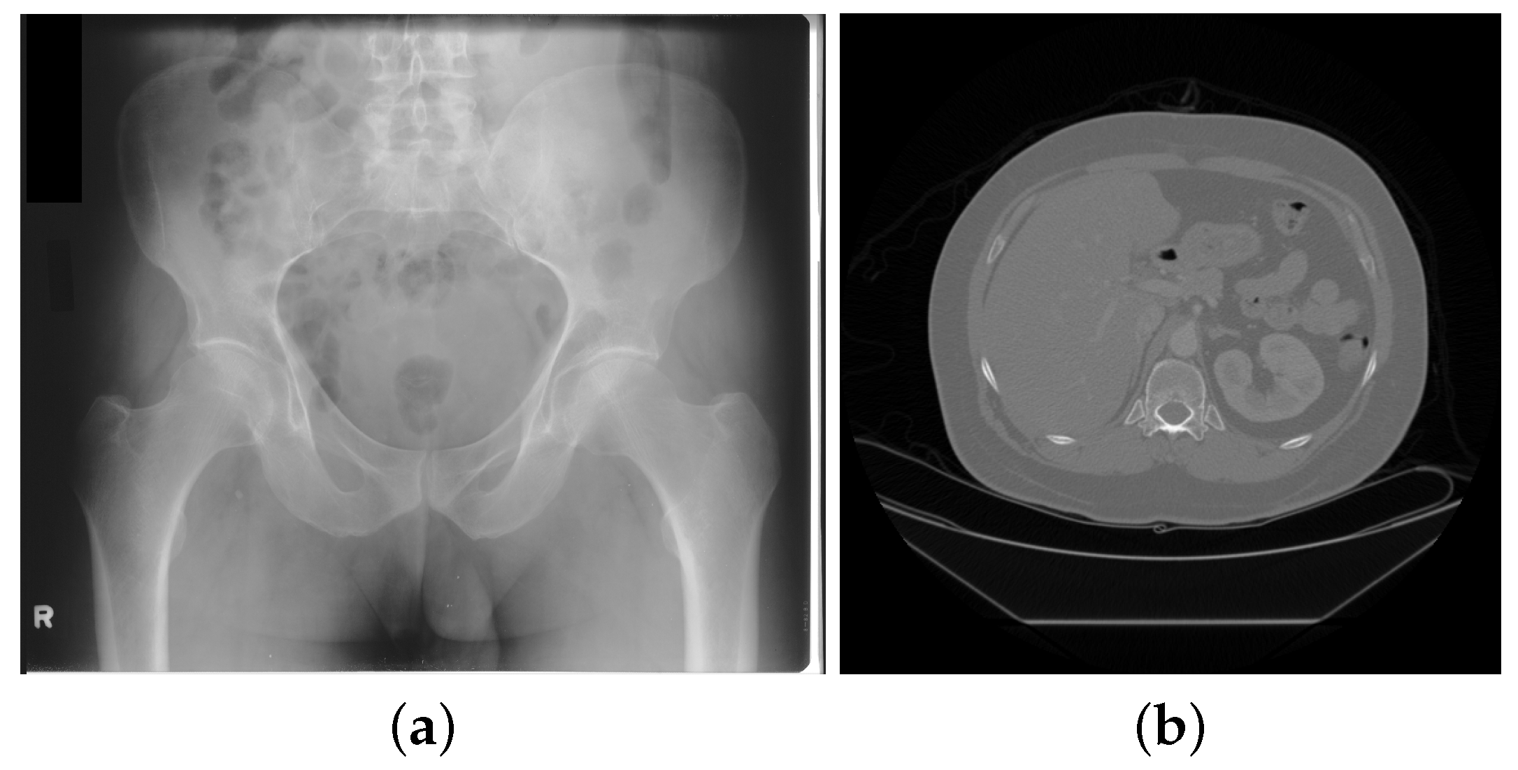
Figure 2.
Three axial MRI images of the same location of the brain obtained using different imaging parameters.
Figure 2.
Three axial MRI images of the same location of the brain obtained using different imaging parameters.

Figure 3.
A digital pathology whole slide image. The 20,000 × 14,000 whole slide image is shown on the left at low magnification and a cropped region is shown on the right at high magnification.
Figure 3.
A digital pathology whole slide image. The 20,000 × 14,000 whole slide image is shown on the left at low magnification and a cropped region is shown on the right at high magnification.
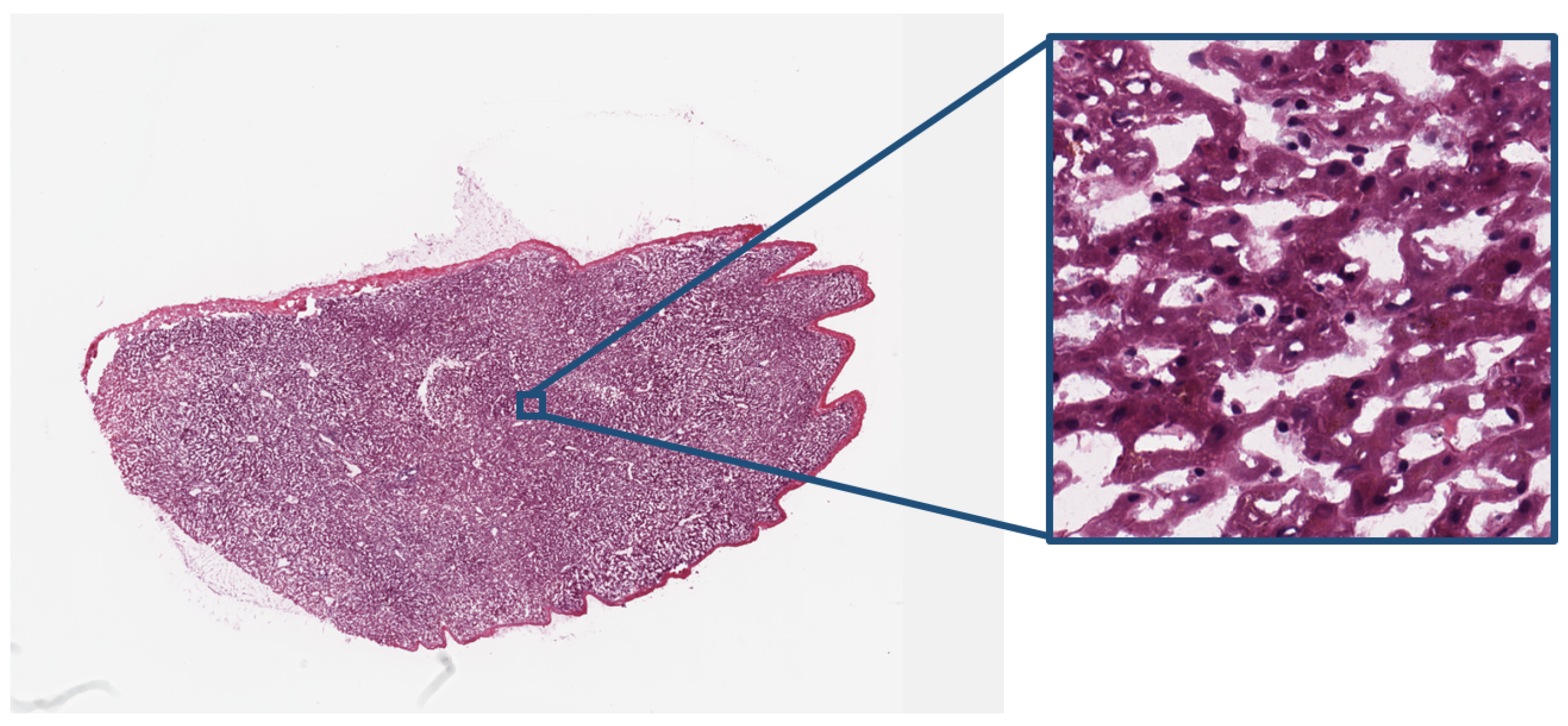
Figure 4.
Baseline JPEG encoder.

Figure 5.
JPEG2000 compression pipeline.

Figure 6.
The prediction template used in JPEG-LS.
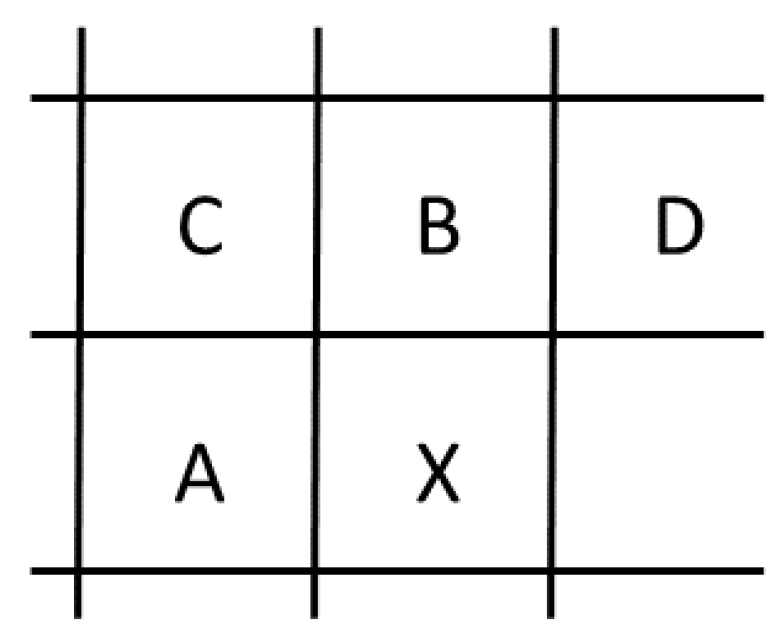
Figure 7.
Simplified block diagram of an encoder capable of generating a compressed bit-stream compliant with the HEVC/H.265 standard.
Figure 7.
Simplified block diagram of an encoder capable of generating a compressed bit-stream compliant with the HEVC/H.265 standard.

Figure 8.
The mean PSNR, SSIM, and HDR-VDP-2 metrics vs. Compression Ratio for CT-COLONOGRAPHY data.
Figure 8.
The mean PSNR, SSIM, and HDR-VDP-2 metrics vs. Compression Ratio for CT-COLONOGRAPHY data.
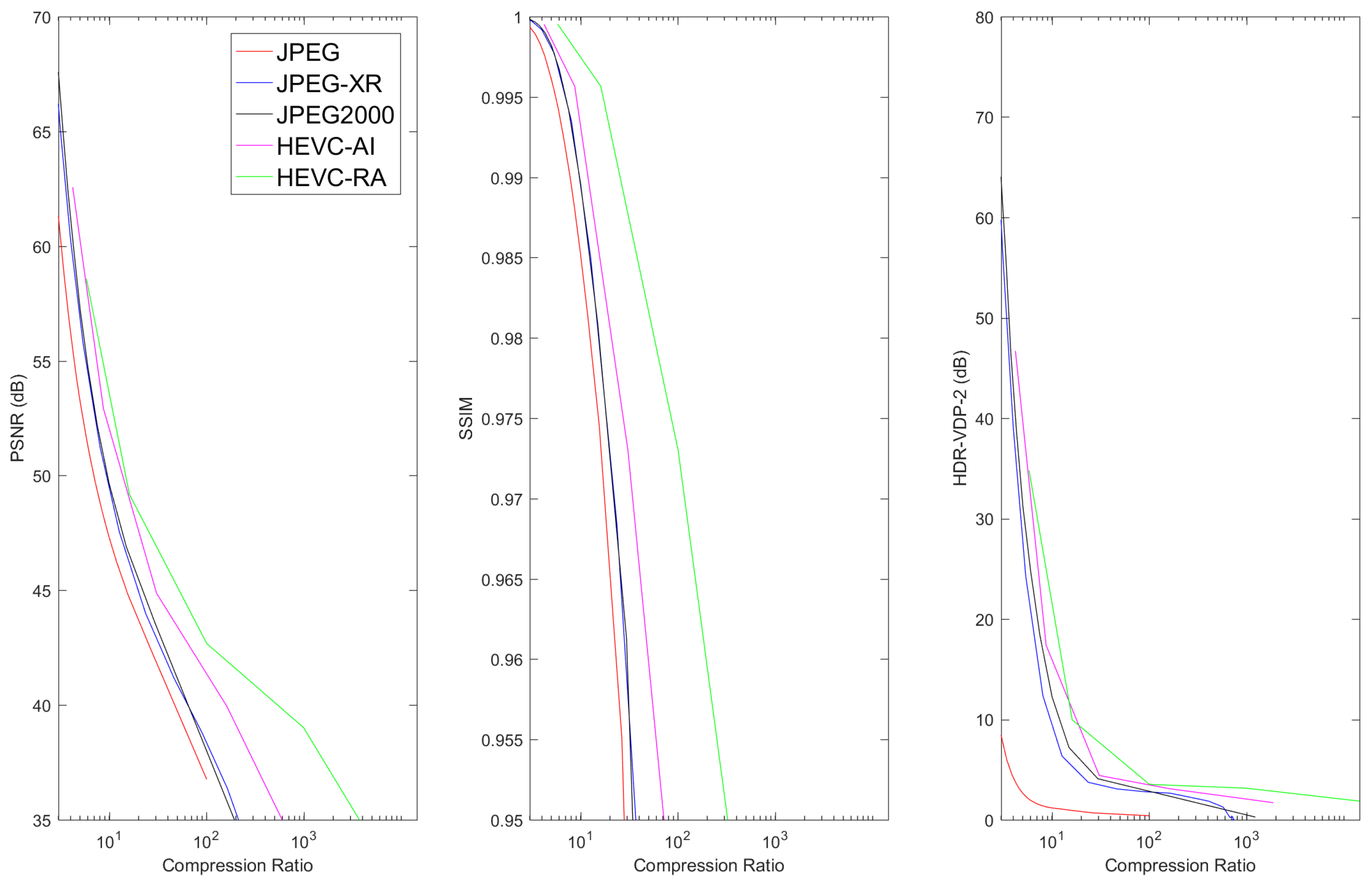
Figure 9.
The mean PSNR, SSIM, and HDR-VDP-2 metrics vs. Compression Ratio for LIDC-IDRI data.

Figure 10.
The mean PSNR, SSIM, and HDR-VDP-2 metrics vs. Compression Ratio for TCGA-BRCA data.
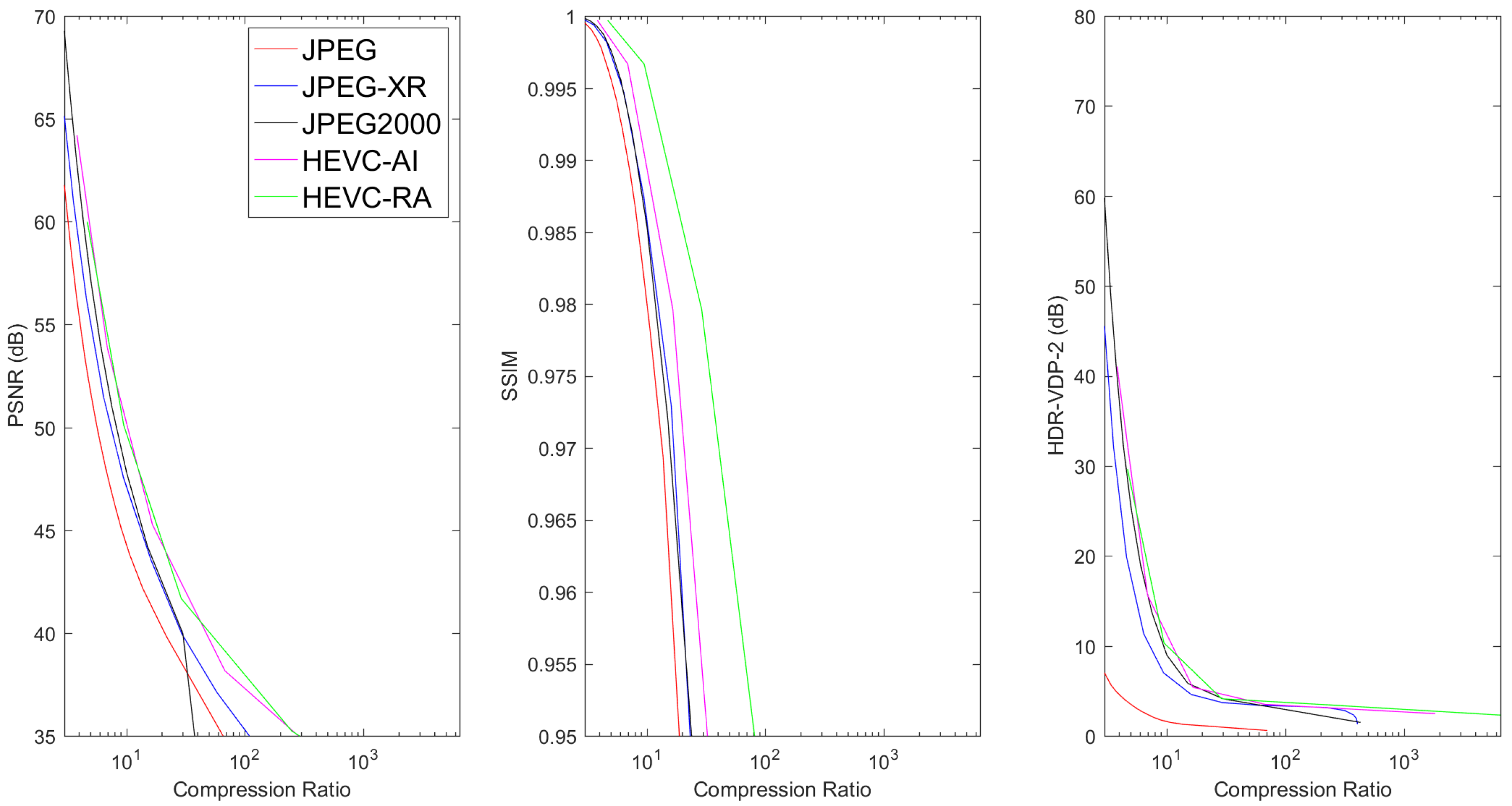
Figure 11.
The mean PSNR, SSIM, and HDR-VDP-2 metrics vs. Compression Ratio for TCGA-GBM data.
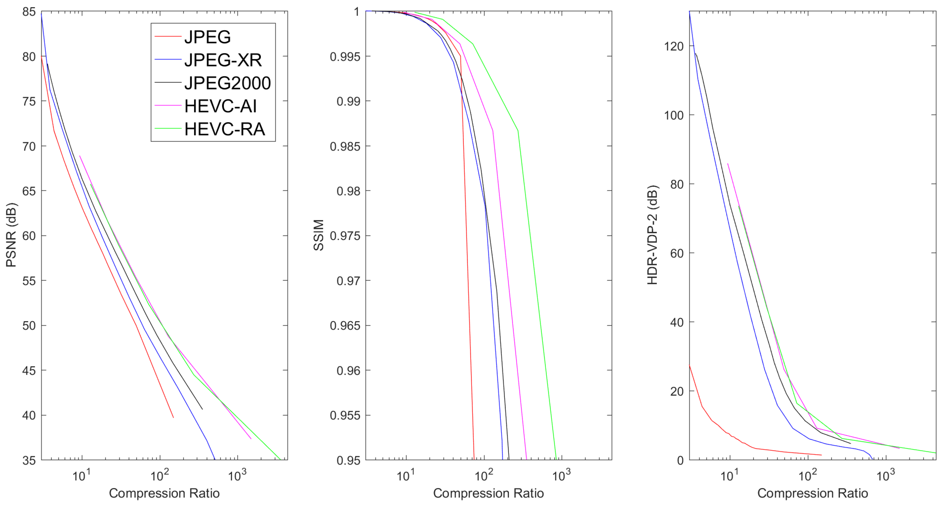
Figure 12.
The mean PSNR, SSIM, and HDR-VDP-2 metrics vs. Compression Ratio for Digital Pathology Data.
Figure 12.
The mean PSNR, SSIM, and HDR-VDP-2 metrics vs. Compression Ratio for Digital Pathology Data.


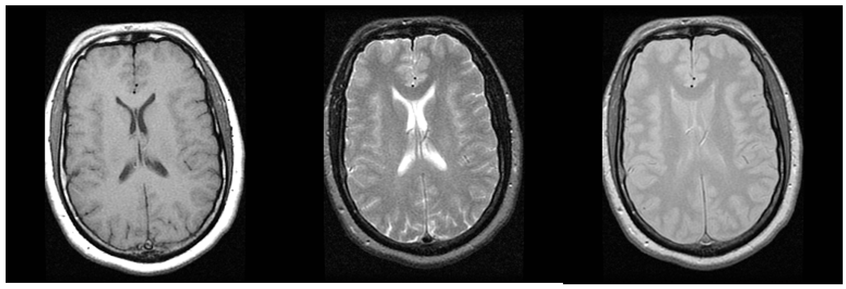
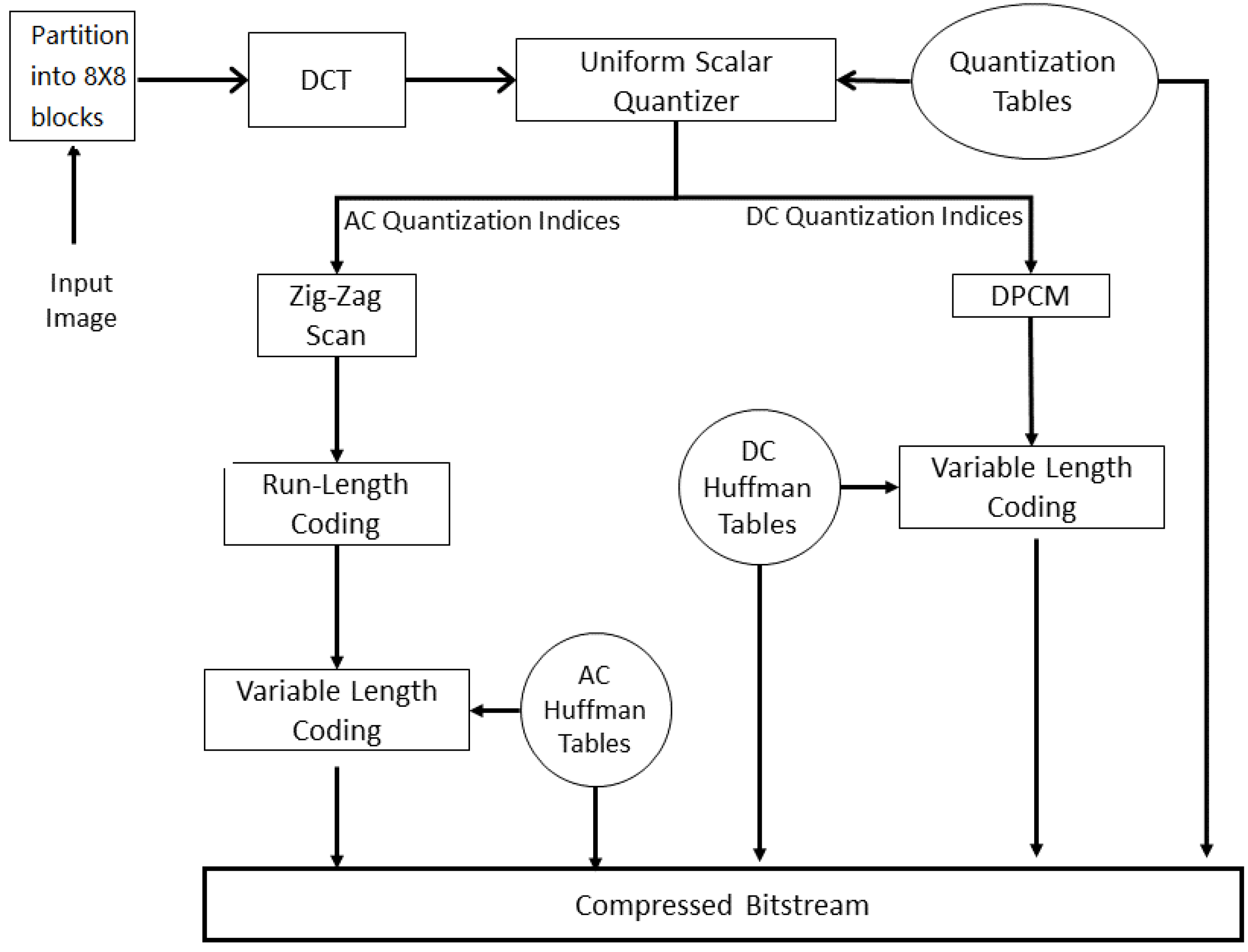
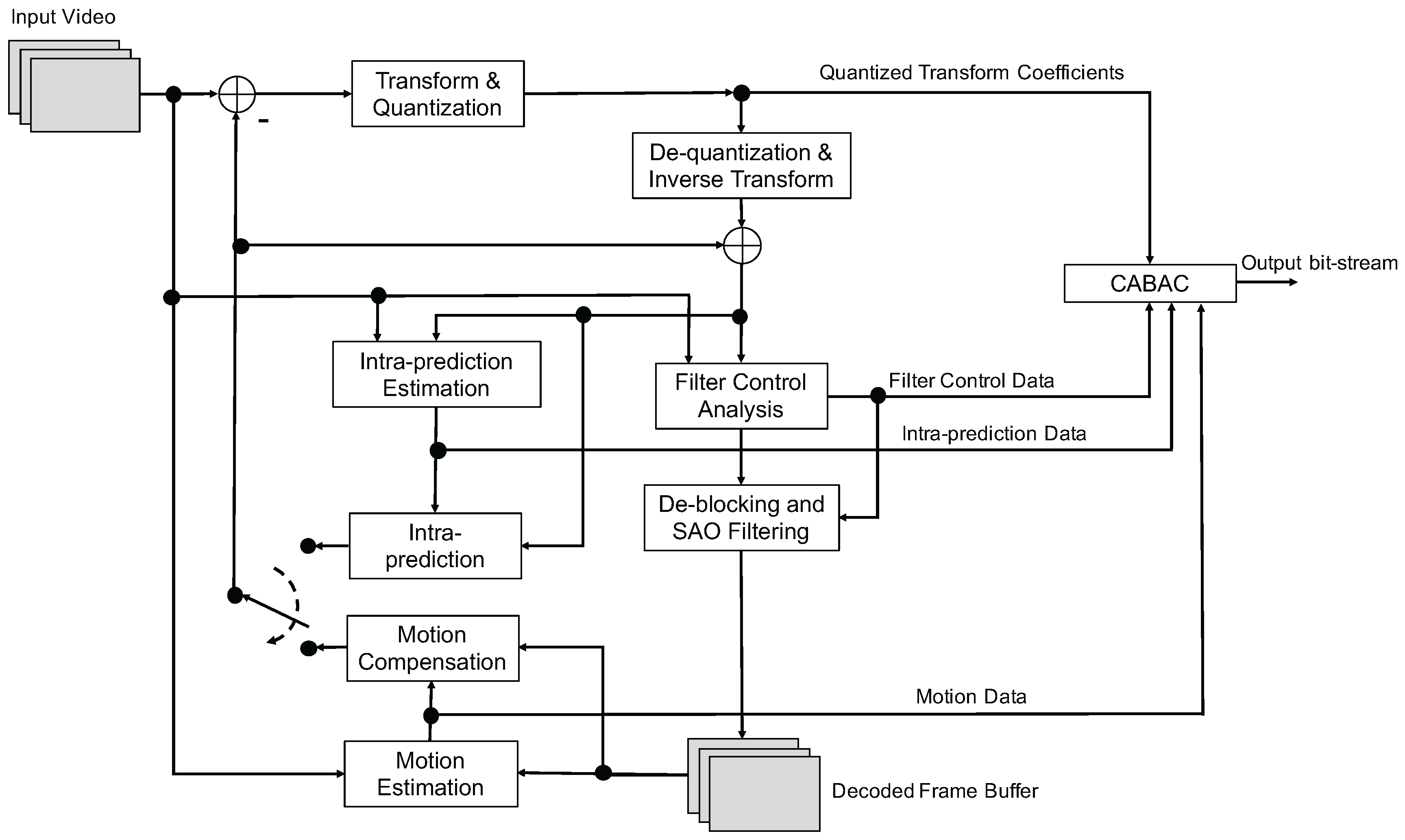
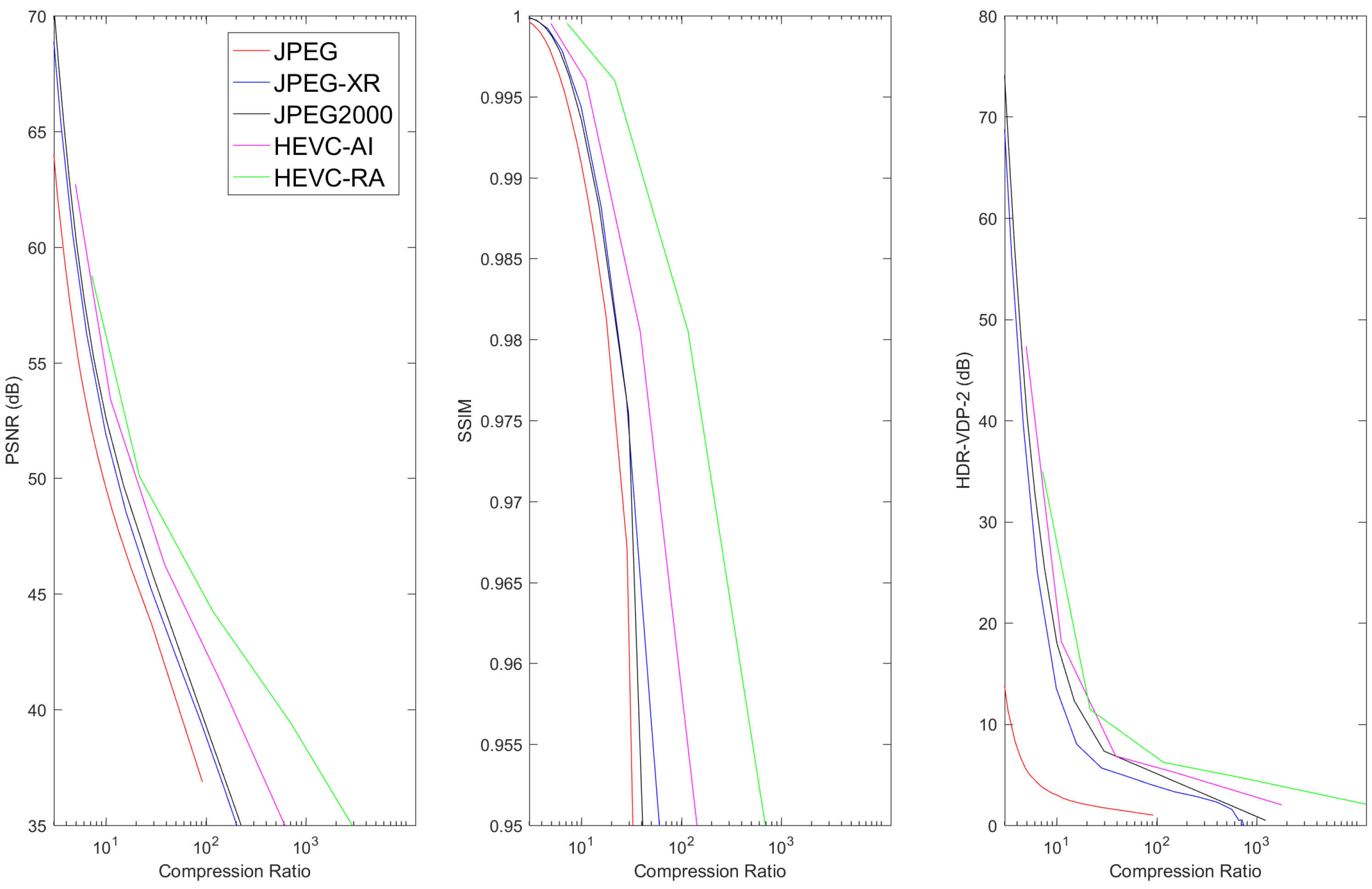
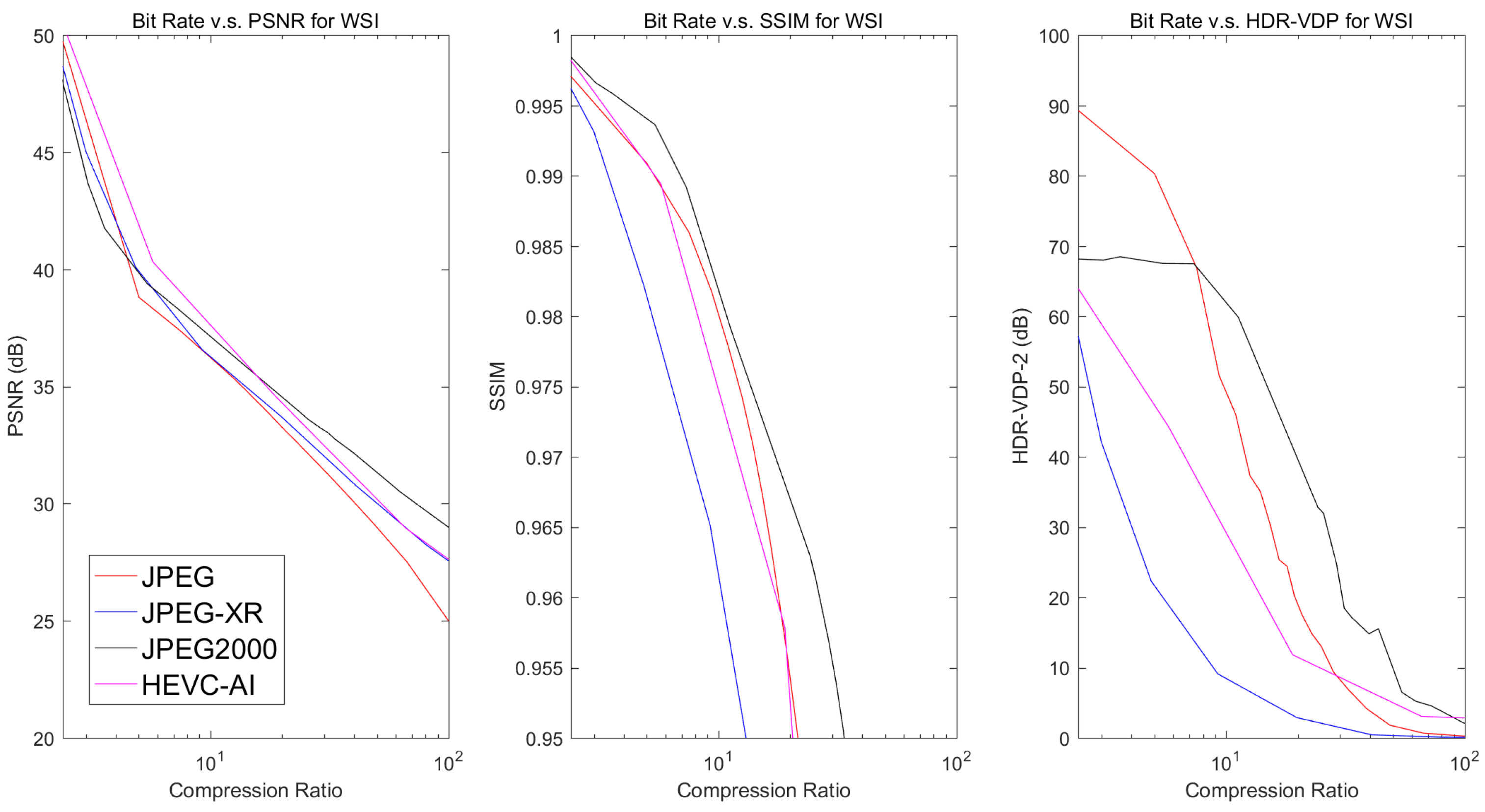
Table 1.
Typical image dimensions and uncompressed file sizes for common medical imaging modalities.
Table 1.
Typical image dimensions and uncompressed file sizes for common medical imaging modalities.
| Modality | Anatomy | Image Dimensions (x, y, z, t) | Bit Depth | Uncompressed File Size |
|---|---|---|---|---|
| Radiography | Chest | (2000, 2500, -, -) | 10–16 bits | 10 MB |
| CT | Abdomen | (512, 512, 500, -) | 12–16 bits | 250 MB |
| Brain | (512, 512, 300, -) | 12-16 bits | 150 MB | |
| Heart | (512, 512, 100, 20) | 12-16 bits | 1 GB | |
| Breast Tomosynthesis | Breast | (2457, 1890, 50, -) | 10–16 bits | 0.4 GB |
| MRI | Abdomen | (512, 512, 100, -) | 12–16 bits | 50 MB |
| Brain | (512, 512, 200, -) | 12–16 bits | 100 MB | |
| Heart | (256, 256, 20, 25) | 12–16 bits | 250 MB | |
| Ultrasound | Heart | (512, 512, -, 50)/s | 24 bits (color) | 38 MB/s |
| PET | Brain | (256, 256, 50, -) | 16 bits | 6 MB |
| Heart | (128, 128, 40, 16) | 16 bits | 1 MB | |
| Digital Pathology | Cells | (30,000, 30,000, -, -) | 24 bits (color) | 2.5 GB |
Table 2.
Lossy compression ratio recommendations by the Royal College of Radiologists [102].
Table 2.
Lossy compression ratio recommendations by the Royal College of Radiologists [102].
| Modality | Compression Ratio |
|---|---|
| Mammography | 20:1 |
| Chest Radiography | 10:1 |
| Skeletal Radiography | 10:1 |
| Ultrasound | 10:1 |
| Digital Angiography | 10:1 |
| CT (all areas) | 5:1 |
| Magnetic Resonance | 5:1 |
| Radiotherapy CT | No lossy compression |
Table 3.
Maximum lossy compression ratios in the Canadian Association of Radiologists standard [103]. Acronyms used in the table: Computed Radiography (CR), Digital Radiography (DR), Computed Tomography (CT), Ultrasound (US), Magnetic Resonance (MR), Nuclear Medicine (NM), JPEG2000 (J2K), Musculoskeletal (MSK). CT denotes CT imaging with a slice thickness of 5 mm or greater and CT denotes CT imaging with a slice thickness of less than 5 mm.
| Modality | ||||||||||||
|---|---|---|---|---|---|---|---|---|---|---|---|---|
| Anatomical | CR/DR | CT | CT | US | MR | NM | ||||||
| Region | JPEG | J2K | JPEG | J2K | JPEG | J2K | JPEG | J2K | JPEG | J2K | JPEG | J2K |
| Angio | - | - | 15:1 | 15:1 | - | - | - | - | 24:1 | 24:1 | 11:1 | 11:1 |
| Body | 30:1 | 30:1 | 15:1 | 10:1 | 12:1 | 12:1 | 12:1 | 12:1 | 24:1 | 24:1 | 11:1 | 11:1 |
| Breast | 25:1 | 25:1 | - | - | - | - | 12:1 | 12:1 | 24:1 | 24:1 | 11:1 | 11:1 |
| Chest | 30:1 | 30:1 | 15:1 | 15:1 | 12:1 | 12:1 | - | - | 24:1 | 24:1 | 11:1 | 11:1 |
| MSK | 30:1 | 20:1 | 15:1 | 15:1 | 12:1 | 12:1 | 12:1 | 12:1 | 24:1 | 24:1 | 11:1 | 11:1 |
| Neuro | - | - | 12:1 | 8:1 | 12:1 | 12:1 | - | - | 24:1 | 24:1 | 11:1 | 11:1 |
| Pediatrics | 30:1 | 30:1 | 15:1 | 15:1 | - | - | 12:1 | 12:1 | 24:1 | 24:1 | 11:1 | 11:1 |
Table 4.
Lossy compression ratio recommendations by the German Röntgen Society [105].
Table 4.
Lossy compression ratio recommendations by the German Röntgen Society [105].
| Modality | Compression Ratio |
|---|---|
| CR/DR (mammography) | 15:1 |
| CR/DR (all areas except mammography) | 10:1 |
| CT (all areas except brain) | 8:1 |
| CT (brain) | 5:1 |
| Magnetic Resonance | 7:1 |
| X-ray Angiography | 6:1 |
| Radio Fluoroscopy | 6:1 |
Table 5.
Description of data sets.
| Database | Modality | Image Dimensions (x, y, z) | Bit Depth |
|---|---|---|---|
| TCIA-COLONOGRAPY | CT Colonography | (512, 512, 426–566) | 12 |
| LIDC-IDRI | CT Lung | (512, 512, 133–280) | 12 |
| TCGA-BRCA | MR Mammography | (256, 256, 148–160) | 12 |
| TCGA-GBM | MR T2 Flair Axial | (384, 512, 25–29) | 12 |
| - | H&E Stained Digital Pathology | (6000, 6000, -) | 24 bits (color) |
Table 6.
Comparison of the lossless compression performances of different methods on different data sets. Average compression ratios as well as the standard deviation of the compression ratios are displayed. The largest average compression ratio for each modality is displayed in bold font.
Table 6.
Comparison of the lossless compression performances of different methods on different data sets. Average compression ratios as well as the standard deviation of the compression ratios are displayed. The largest average compression ratio for each modality is displayed in bold font.
| Modality | Compression Standard | Compression Ratio |
|---|---|---|
| CT Colonography | JPEG-LS | 1.89 ± 0.1089 |
| Lossless JPEG-XR | 1.79 ± 0.0869 | |
| Lossless JPEG2000 | 1.86 ± 0.1042 | |
| HEVC AI | 1.64 ± 0.0897 | |
| HEVC RA | 1.87 ± 0.1315 | |
| CT Lung | JPEG-LS | 2.08 ± 0.3195 |
| Lossless JPEG-XR | 1.94 ± 0.2571 | |
| Lossless JPEG2000 | 2.02 ± 0.3160 | |
| HEVC AI | 1.84 ± 0.2739 | |
| HEVC RA | 2.10 ± 0.3217 | |
| MR Mammography | JPEG-LS | 2.06 ± 0.2520 |
| Lossless JPEG-XR | 1.72 ± 0.1401 | |
| Lossless JPEG2000 | 2.01 ± 0.2406 | |
| HEVC AI | 1.77 ± 0.2357 | |
| HEVC RA | 2.03 ± 0.2504 | |
| MR T2 Flair Axial | JPEG-LS | 2.75 ± 0.2267 |
| Lossless JPEG-XR | 2.85 ± 0.2206 | |
| Lossless JPEG2000 | 2.91 ± 0.2463 | |
| HEVC AI | 2.26 ± 0.1818 | |
| HEVC RA | 2.51 ± 0.1955 | |
| Digital Pathology | JPEG-LS | 1.72 ± 0.0786 |
| Lossless JPEG-XR | 1.72 ± 0.0497 | |
| Lossless JPEG2000 | 1.76 ± 0.0674 | |
| HEVC AI | 1.49 ± 0.0905 |
© 2017 by the authors. Licensee MDPI, Basel, Switzerland. This article is an open access article distributed under the terms and conditions of the Creative Commons Attribution (CC BY) license (http://creativecommons.org/licenses/by/4.0/).
Share and Cite
MDPI and ACS Style
Liu, F.; Hernandez-Cabronero, M.; Sanchez, V.; Marcellin, M.W.; Bilgin, A. The Current Role of Image Compression Standards in Medical Imaging. Information 2017, 8, 131. https://doi.org/10.3390/info8040131
AMA Style
Liu F, Hernandez-Cabronero M, Sanchez V, Marcellin MW, Bilgin A. The Current Role of Image Compression Standards in Medical Imaging. Information. 2017; 8(4):131. https://doi.org/10.3390/info8040131
Chicago/Turabian StyleLiu, Feng, Miguel Hernandez-Cabronero, Victor Sanchez, Michael W. Marcellin, and Ali Bilgin. 2017. "The Current Role of Image Compression Standards in Medical Imaging" Information 8, no. 4: 131. https://doi.org/10.3390/info8040131
Note that from the first issue of 2016, this journal uses article numbers instead of page numbers. See further details here.