MR Brain Image Segmentation: A Framework to Compare Different Clustering Techniques


1
Department of Computer Science, University of Bari Aldo Moro, 70125 Bari, Italy
2
Department of Electrical and Information Engineering, Polytechnic of Bari, 70125 Bari, Italy
*
Author to whom correspondence should be addressed.
†
Current Address: Via Orabona, 4-70125 Bari, Italy.
Information 2017, 8(4), 138; https://doi.org/10.3390/info8040138
Submission received: 8 October 2017
/
Revised: 1 November 2017
/
Accepted: 1 November 2017
/
Published: 4 November 2017
(This article belongs to the Special Issue Fuzzy Logic for Image Processing)
Abstract
:In Magnetic Resonance (MR) brain image analysis, segmentation is commonly used for detecting, measuring and analyzing the main anatomical structures of the brain and eventually identifying pathological regions. Brain image segmentation is of fundamental importance since it helps clinicians and researchers to concentrate on specific regions of the brain in order to analyze them. However, segmentation of brain images is a difficult task due to high similarities and correlations of intensity among different regions of the brain image. Among various methods proposed in the literature, clustering algorithms prove to be successful tools for image segmentation. In this paper, we present a framework for image segmentation that is devoted to support the expert in identifying different brain regions for further analysis. The framework includes different clustering methods to perform segmentation of MR images. Furthermore, it enables easy comparison of different segmentation results by providing a quantitative evaluation using an entropy-based measure as well as other measures commonly used to evaluate segmentation results. To show the potential of the framework, the implemented clustering methods are compared on simulated T1-weighted MR brain images from the Internet Brain Segmentation Repository (IBSR database) provided with ground truth segmentation.
1. Introduction
Medical image analysis plays a crucial role in modern diagnosis. Thus, computer-based image analysis is becoming an important field, with an increasing reliance on it by the biomedical community. Diagnostic imaging is an invaluable tool in medicine today. Magnetic Resonance Imaging (MRI), Computed Tomography (CT), digital mammography and other imaging modalities provide effective means for non-invasive analysis of the anatomy of a subject. Then, computer algorithms designed for the delineation of anatomical structures and other regions of interest are key components in assisting or even automating specific medical tasks.
Image segmentation is an essential and crucial process for facilitating the delineation, characterization, and visualization of a Region Of Interest (ROI) in any medical image, because its output affects all subsequent processes of image analysis.
Medical images are difficult to segment, mainly due to the complexity of the anatomical features involved. The ROI may not be separable from its surroundings due to gray level inconsistency and the absence of strong edges along its border. The images typically contain noise, which may alter the intensity of a pixel such that its classification becomes uncertain. A single tissue class may show non-uniformity of intensity over the extent of the image. Uncertainty also occurs due to the observer variability at the expert level. Segmentation algorithms should be able to cope with these challenges. Segmentation methods vary widely depending on the specific application, the imaging modality and other factors. Currently, there is no unique segmentation method that yields acceptable results for every medical image.
Among medical imaging modalities, MRI is one of the safest methods for producing data with high spatial resolution, and it is also a low-risk, non-invasive modality in comparison to other diagnostic imaging techniques [1]. For this reason, the majority of research in medical image segmentation pertains to its use for MR images, and there are many methods available for MR image segmentation.
In particular, the segmentation of MR brain images has obtained significant focus in the field of biomedical image processing. It plays an important role in both clinical practice and neuroscience research, with applications in the field of bio-medical analysis, such as identification of tumors, classification of tissues and blood cells, multi-modal registration [2], etc. Furthermore, the ability to segment and quantify brain tissues and anatomical structures has received increasing importance in the study of brain development [3,4], and its pathologies such as neurodegeneration [5,6], and dementia [7,8], as well as in the assessment of neurological [9,10] and psychiatric disorders [11,12].
A brain image mainly consists of three regions: Gray Matter (GM), White Matter (WM) and Cerebrospinal Fluid (CSF) [13]. Segmentation of a brain image aims to identify these three regions by exploiting the gray level distribution of pixels. Due to the complex structure of brain tissues in the brain images, manual segmentation is a difficult and time-consuming process. Therefore, there is a strong need to have efficient computer-based systems that can identify accurately the boundaries of brain tissues along with low interaction with the human expert.
Various automatic techniques have been proposed for segmentation of MR brain images. Their basic idea is to detect discontinuity among pixels of different regions or similarity among pixels of the same region. One category includes algorithms for detecting isolated points, lines or edges, like thresholding [14], edge-based detection [15] and region growing [16]. Thresholding techniques are effective when the histograms of the ROIs and background are clearly identifiable. However, for brain images, these techniques give inaccurate segmentation results since the distribution of pixels in the brain image is very complex. Edge-based methods rely heavily on detection of boundaries in the image. However, when applied to brain images, they often result in the wrong detection of boundaries due to the complex gray level distribution of GM, WM and CSF pixels.
Another category of segmentation methods includes algorithms of region growing, region splitting and merging. Region growing techniques use the homogeneity and connectivity criteria for segmentation; hence, a region growing algorithm merges pixels based on certain criteria. Region-based segmentation algorithms typically rely on the homogeneity of the image intensities in the regions of interest, which often fail to provide accurate segmentation results due to the intensity inhomogeneity. In [17], a region-based method for image segmentation, which is able to deal with intensity inhomogeneities in the segmentation, is proposed.
Other common segmentation methods are active contour models, also called snakes, used for delineating an object outline from a possibly noisy 2D image. In [18], an edge-based active contour model using the inflation/deflation force is proposed. The method allows active contour nodes to be moved to find object boundaries in a digital image. Experiments on MRI medical images show that the method is of major practical significance if the analyzed images contain weak boundaries and/or strong noise at the same time. In [19], an active contour model is proposed to segment images with intensity inhomogeneities. This method uses Gaussian kernel filtering to regularize the level set function after each iteration. Experiments show that the method achieves similar results to the local binary fitting energy method, but in a computationally more efficient way.
Among pixel-based approaches, clustering methods are the most widely used for image segmentation [20]. Clustering is the process of grouping a set of points (feature vectors) into subsets (called clusters) so that points in the same cluster are similar in some sense [21]. Several types of clustering methods have been discussed in the literature like expectation–maximization [1], K-means and fuzzy clustering techniques [22,23], which allow image pixels to belong to more than one class. Among fuzzy clustering techniques, Fuzzy C-Means (FCM) is the most widely-used technique [24]. It aims at minimizing an objective function according to some criteria. It permits one data point to belong to more than one cluster defined by a membership matrix.
In the last decade, clustering-based approaches received great interest in the domain of medical imaging. A huge number of papers has been proposed in the literature concerning the application of clustering methods to the segmentation of medical images such as MR breast images [25,26], microscopic blood cell images [27,28] and X-ray images [29,30]. In particular, many works demonstrate the effectiveness of clustering for segmentation of MR brain images in order to detect GM, WM and GSF regions [31,32,33,34].
Despite the huge number of clustering techniques proposed for medical image segmentation, a general framework for assessing the validity of the different segmentation methods is missing. Indeed, there are many works in the remote sensing field for segmentation quality assessment, including tools for tuning segmentation parameter values [35,36]. Proposed frameworks in the field of medical images enable only visual quality inspection of the segmentation results [37]. Only very few studies propose frameworks for quantitative evaluation of MR image segmentation [38], but no available software tool is developed. Hence, there is a need for open-source validation tools to assess the reliability of segmentation results obtained by different clustering methods applied to MR images.
To this aim, in this work, we present a framework to aid the clinicians in the identification of the best segmentation results for their specific task. The framework includes different clustering methods and some evaluation metrics to assess the quality of the results. Specifically, for each method, the framework enables easy definition of specific running parameters and enables comparison of the segmentation results. The framework includes specific pixel-based approaches for MR image segmentation that are based on clustering and enables comparison of segmentation results obtained by different clustering methods. Comparison is made not only qualitatively, through visual inspection of segmented images, but also quantitatively by means of the evaluation method proposed in [39]. This method is based on information theory, and it uses entropy as the basis for measuring the uniformity of pixel luminance within a segmentation region. The evaluation method provides a relative quality score that can be used within the framework to compare different segmentations of the same image.
2. The Image Segmentation Framework
Classically, image segmentation is defined as the partitioning of an image into non-overlapping regions, which are homogeneous with respect to some characteristic such as intensity or texture [40,41,42]. In general, image segmentation has a two-fold goal:
- (a)
- Partitioning: divide into regions/sequences with coherent internal properties;
- (b)
- Grouping: identify sets of coherent tokens in the image.
The goal of segmentation is also to simplify and/or change the representation of an image from a low-level (rough data) into a medium-level representation (image segmented into regions) that is more understandable and suitable for further analysis. An image is a collection of measurements in two-dimensional (2D) or three-dimensional (3D) space. In medical images, these measurements or image intensities can be radiation absorption in X-ray imaging, acoustic pressure in ultrasound or RF signal amplitude in MRI.
Given an image I, the segmentation problem is to determine the regions whose union is the entire image I, namely:
where for , and each is connected.
When the constraint that regions be connected is not considered, then the process of determining the regions is called pixel classification, and the regions are called classes. Pixel classification rather than classical segmentation is often a desirable goal in medical images, particularly when disconnected regions belonging to the same tissue class need to be identified. Determination of the total number of classes K in pixel classification is a difficult problem [43] especially when prior knowledge about the anatomy depicted in the image is missing.
The framework presented in this work is intended to aid the clinician in the application of different clustering methods for image segmentation. It includes four state-of-art clustering algorithms, namely the K-means, the fuzzy C-means, the spatial fuzzy C-means and the kernelized FCM algorithm. The framework allows the user to set the parameters of each method and to compare the obtained segmentation results using some evaluation metrics.
The core of the tool is based on the ImageJ environment (imagej.nih.gov/ij/), which is an open source software for image processing extended with new functionalities. The main steps accomplished are the following:
- choosing the image
- choosing the color space
- choosing the segmentation method
- setting the running parameters of the specific method
- visualizing the segmented image
- computing the evaluation metrics
More in detail, the main components of the tool are the following:
- User work section: This component gives the user the possibility to access the primary functions of the tool, which are the clustering method section and the evaluation section.
- Method section: For each implemented method, the user can configure its parameters such as color space conversion, number of cluster, maximum number of iterations, stopping condition and visualization mode.
- Evaluation section: The segmentation results can be evaluated both qualitatively and quantitatively. Qualitative evaluation is made by visualization of the segmented image compared to the ground truth image. Quantitative evaluation is made by computing the metrics described in Section 4.
The tool offers different visualization modes for displaying the segmented image, namely the regions can be labeled in different ways:
- by the cluster centroid color: Each point of a cluster is labeled with the color of its centroid (in the case of color conversion, the color space is converted back to RGB);
- by a gray level: Each pixel is labeled with the number of the cluster it belongs to, and the range is stretched in 0–255;
- by a random RGB color: A random RGB value is generated for each cluster;
- by a binary stack: The clustering is represented as a stack of binary images. Each binary image represents a cluster; each pixel shows a hard cluster membership. Thus, it is possible to extract cluster regions from the original image by performing an AND operation between a slide of the stack and the original image.
- by using a fuzzy stack: A stack of gray level images is used to show the membership values of each pixel to each cluster. Each pixel represents the soft cluster membership value of that pixel in the original image according to the currently selected cluster.
Moreover, the tool enables selection of general parameters such as number of clusters, maximum number of iterations, stopping criterion and tolerance value used to stop the algorithm, initialization criterion for the centers and the membership matrix and randomized seed used to initialize a random number sequence.
In the following sections, the implemented clustering methods and the adopted evaluation metrics are briefly described.
3. Clustering Methods
3.1. K-means
The K-means algorithm [44] is the major example of partitional crisp clustering that assumes each data point to belong exactly to one cluster. It aims to partition N points into K partitions (clusters) in which each point belongs to the cluster having the nearest mean. Even though K-means was first proposed over 50 years ago, it is still by far the most used clustering algorithm for its simplicity of implementation and its effectiveness. When applied to image segmentation, the K-means algorithm clusters image pixels (features could be the color or the luminance of a pixel) by iteratively computing a mean intensity for each cluster and segmenting the image by associating each pixel to the cluster with the closest mean [21].
Let be the set of pixels and be the set of cluster means (centers). A partition of the image I into K clusters can be represented by mutually disjoint sets such that . To represent the partition of I into K clusters, a binary membership matrix is used, where if , otherwise, for and .
The objective of the K-means algorithm is to minimize the distance among pixels inside the same cluster and to maximize the distance between clusters. This is obtained by minimizing the following objective function:
where is the Euclidean distance.
The main steps of the K-means algorithm for image segmentation are:
- Fix the number of clusters K, and initialize the cluster centers (), either randomly or based on some heuristic;
- Assign each pixel to the cluster that minimizes the distance between the pixel and the cluster center;
- Re-compute the cluster centers by averaging all of the pixels in the cluster, namely:
- Repeat Steps 2 and 3 until convergence is attained (i.e., the assignment of pixels to clusters does not change)
One main issue of the K-means algorithm is that the clustering result depends strongly on the initialization of the cluster centers and on the number of clusters. Besides, K-means is a local optimum search technique that usually converges to a local minimum, and it does not take pixel distribution in consideration.
3.2. Fuzzy C-Means
Unlike crisp clustering methods, which force pixels to belong exclusively to one cluster, fuzzy clustering methods allow pixels to belong to multiple clusters with varying degrees of membership, thus enabling vague or fuzzy borders between different clusters. There has been considerable interest in the past few years in the use of fuzzy segmentation methods, which retain more information from the original image than crisp segmentation methods [45,46,47]. The main example of the fuzzy clustering algorithm is the fuzzy version of the K-means called Fuzzy C-Means (FCM) [24].
FCM is a partition clustering method based on the minimization of the following objective function:
where is the distance between the point and the cluster center , m is the fuzziness parameter, K is the number of clusters, N is the number of data points and is the membership degree of belonging to the cluster k, calculated as follows:
for , . Using the fuzzy membership matrix , a new position of the k-th centroid is calculated as:
with the constraint . The fuzziness parameter is a scalar weighting exponent that controls the fuzziness degree of the clustering process. The larger is its value, the fuzzier is the partition. If this parameter has value , the FCM approaches the crisp K-means algorithm, the membership values being only zero or one. When m approaches infinity, the mass center of the dataset is the only solution of FCM. The most common choice for m is , which has been proven to be suitable also for MR brain image segmentation [48].
Minimization of (3) is obtained by iteratively computing membership values according to Equation (4) and cluster centers as in Equation (5). The main steps of the FCM algorithm are the following:
- Fix the number of clusters K and initialize the cluster centers (), either randomly or based on some heuristic;
- Compute membership values using Equation (4)
- Re-compute the cluster centers using Equation (5)
- Repeat Steps 2 and 3 until convergence is attained (i.e., the assignment of pixels to clusters does not change)
The parameters required to run the FCM algorithm are the number of clusters K and the fuzziness parameter m. Our framework enables the selection of these parameters.
The FCM algorithm has been used widely for the segmentation of MR images [49,50,51]. The FCM method, however, does not address the spatial intensity inhomogeneity artifact induced by the radio-frequency coil in MR images [52,53]. To deal with the inhomogeneity problem, many algorithms have been proposed by adding correction steps before segmenting the image [54,55] or by modeling the image as the product of the original image and a smooth varying multiplier field [1,45]. More recently, spatial information has been embedded into the original FCM algorithm to better segment the images [56,57]. The framework presented in this paper includes one example of spatial FCM that is briefly described in the following section.
3.3. Spatial FCM
From Equation (3), it can be observed that FCM does not incorporate any spatial dependencies between pixels. This may degrade the overall segmentation result, because neighboring regions may be highly correlated, and thus, they should belong to the same cluster. When applied to image segmentation, clustering should take into account the spatial information of pixels. To this aim, several spatial variants of the FCM have been proposed. Among these, we consider the Spatial FCM (SFCM) proposed in [58] and applied in [59] to biomedical image segmentation. The SFCM uses a spatial function defined as:
where represents a neighbor of the pixel in the spatial domain. Just like the membership function, the spatial function represents the membership degree of pixel belonging to the j-th cluster. The spatial function of a pixel for a cluster is large if the majority of its neighbors belongs to the same clusters. The spatial function modifies the membership function of a pixel according to the membership statistics of its neighbors as follows:
where p and q are parameters to control the relative importance of both functions. The iterative scheme of the SFCM is the same as in FCM, but Step 2 includes three sub-steps. The first one is the same as in standard FCM, i.e., to calculate the membership values using Equation (4). In the second sub-step, the membership information of each pixel is mapped to the spatial domain, and the spatial function is computed from that using Equation (6). Then, the new membership values are computed according to (7). The SFCM iteration proceeds by updating cluster centers according to (5) as in FCM.
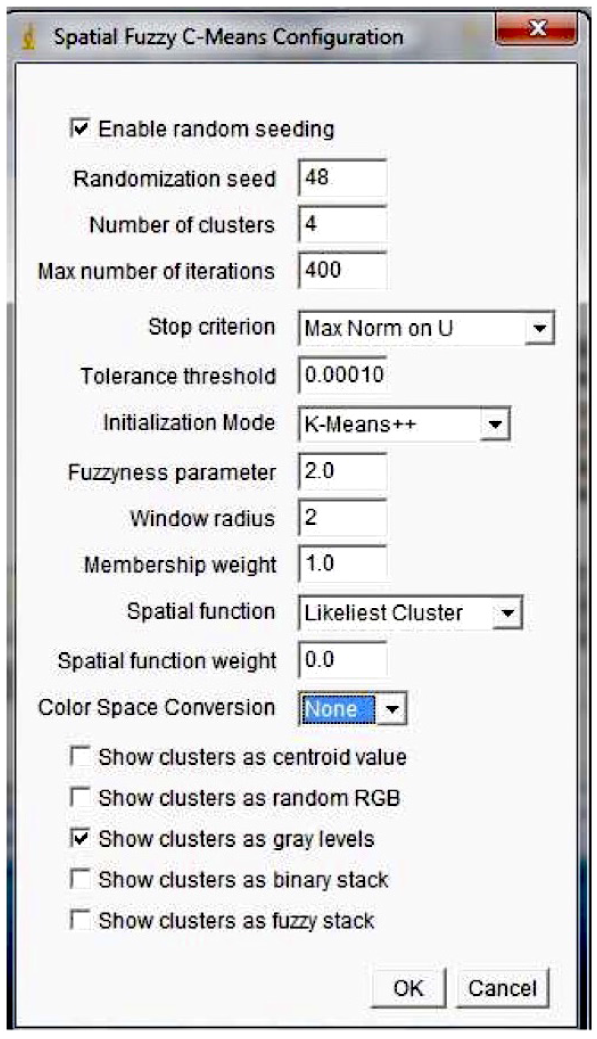
Specific parameters that can be set for this algorithm are:
- : fuzziness parameter used to control the fuzziness; if m is near one, the results are similar to those obtained by K-means
- p and q: parameters used to control the relative importance of membership and spatial functions
- Radius r: the spatial function is evaluated on a window centered on the pixel
Figure 1 shows the interface of our framework that enables the user to define such parameters.
3.4. Kernelized FCM
In recent years a number of powerful kernel-based learning methods have been proposed [60] that work to construct a nonlinear version of a linear algorithm using the so-called “kernel trick” or kernel substitution. This consists of using a (implicit) nonlinear map, from the data space to the mapped feature space so that an input data space X with low dimension is mapped into a potentially much higher dimensional feature space F in order to turn the original nonlinear problem in the input space into potentially a linear one in a rather high dimensional feature space. A kernel in the feature space can be represented as a kernel function K defined as:
where denotes the inner product operation. There are different commonly-used kernel functions in the literature, such as the Gaussian Radial Basis Function (GRBF) kernel, polynomial kernel and sigmoid kernel [60].
The kernel method has also been applied to clustering. In particular, in [61], a Kernelized version of fuzzy C-means (KFCM) is proposed and applied to the segmentation of MR images. It is realized by replacing the original Euclidean distance in the FCM algorithm with a kernel-induced distance. The KFCM minimizes the following objective function:
Using the GRBF kernel, we have ; hence, we obtain the following simplified expression:
and the objective function (8) can be rewritten as:
Similarly to the standard FCM algorithm, the objective function can be iteratively minimized by using the following update formulas:
and:
The KFCM algorithm follows the same iterative scheme as FCM.
4. Evaluation Metrics
The validation process is an important step to define the reliability and reproducibility of a given brain MRI segmentation method. Often, the results of segmentation methods are evaluated only visually and qualitatively. Such an approach is either subjective or tied to particular applications. Conversely, it is desirable to judge the performance of a segmentation method objectively; hence, qualitative evaluation cannot be used as a means to compare the performance of different segmentation techniques.
Typically for quantitative validation purposes, the segmented brain images are compared to the corresponding ground truth, and an evaluation metric is calculated. For instance, the number of pixels that have been correctly segmented is divided by the total number pixels in the brain. Common measures used for quantitative evaluation of segmentation methods are accuracy, sensitivity and specificity. The accuracy of the segmentation method is computed as the rate of correctly classified pixels over all pixels. Given a tissue T (GM, WM, CSF), it is defined as:
where
- (True Positive) is the number of pixels that belong to tissue T in the ground truth image and are correctly classified as tissue T in the segmented image;
- (False Negative) is the number pixels that are classified as tissue T in the ground truth image, but classified as different tissues in the segmented image;
- (True Negatives) is the number of pixels that are classified as different tissues both in the segmented and ground truth images;
- (False Positives) is the number of pixels incorrectly classified as tissue T in the segmented image compared to the ground truth image.
Sensitivity refers to the ability of a clustering method to accurately identify the tissue regions in the segmented image. It is defined as:
The specificity reflects the ability of the clustering method to accurately identify the non-tissue regions. It is defined as:
Other measures usually considered to evaluate segmentation are the Dice Similarity Coefficient (DSC) and the Jaccard Similarity (JS) value. DSC is a statistical validation metric that was proposed in [62] to evaluate the accuracy of segmentation methods. The DSC measure describes the overlap between the segmented and ground truth images using the following formula:
The JS metric is defined as:
where G is the ground-truth image and S is the segmented image. High values of indicate that the segmented regions match the ground truth regions well. The above metrics do not always express completely the quality of a segmentation method. A good segmentation evaluation should maximize the uniformity of pixels within each segmented region and minimize the uniformity across the regions. Consequently, a natural characteristic to incorporate into a segmentation evaluation metric is a measure of the disorder within a region. Along with this idea, in [39], the concept of entropy is used to measure the disorder within regions of a segmented image. Given a segmented image , where is a region of the image, we indicate by v a specific feature used to describe the pixels in region and define as the set of all possible values associated with feature v in region and as the number of pixels that have a value of m for feature v. The entropy for region is defined as:
where denotes the area of region .
Here, we consider v to be the luminance of pixels and simplify to . Hence, from an information coding theory point of view, the quantity represents the probability that a pixel in region has a luminance value of m. Thus, is the number of bits per pixel needed to encode the luminance for region , given that the region is known. Finally, we define the expected region entropy of image I as the expected entropy across all regions where each region has weight (or probability) proportional to its area. That is, the expected region entropy of segmented image I is:
where is the area (as measured by the number of pixels) of the entire image. When each region has very uniform luminance, then will be small. Besides, when all pixels in a region have the same value, then the entropy for the region will be zero. Since an over-segmented image will have a very small value of , this value should be combined with another term that penalizes segmentations having a large number of regions. In order to fully encode the information in a segmented image, we should not only encode the luminance value of a pixel within a region (i.e., the region entropy), but also a representation for the segmentation itself, i.e., we should specify the region for each pixel. In [39] the authors introduce the layout entropy as a measure to encode the region for each pixel, defined as:
Using a coding theory framework, one can view as the probability that a pixel in the image belongs to region j under a probabilistic assumption that each pixel is independently selected to be in region j with probability . Hence, represents the number of bits for specifying a region for each pixel.
While the expected region entropy provides an estimate of the average disorder within regions in a segmented image and it generally decreases with the number of regions, the layout entropy increases with the number of regions. Hence, the two factors and can be used to counteract the effects of over-segmenting or under-segmenting when evaluating the effectiveness of a given segmentation. By additively combining both the layout entropy and the expected region entropy, in [39], the entropy-based evaluation function E is introduced to measure the effectiveness of a segmentation method. It is defined as:
When the image is maximally segmented (with one pixel per region) E is not minimized, since in such a case, the layout entropy becomes very large. Furthermore, when the image is under-segmented (with very few regions) E is not minimized since the expected region entropy will be high. As desired, the measure E balances these two factors.
5. Application and Results
In this section, we present some comparative results of MR image segmentation using the clustering methods implemented in the proposed framework. A preliminary version of the tool is available at [63]. The framework is developed in Java as a plugin for ImageJ (http://imagej.nih.gov), a public-domain Java image processing program inspired by NIH image for Macintosh. The functions provided by ImageJ built-in commands can be extended by user-written code in the form of macros and plugins. Figure 2 shows an excerpt of code of our framework that summarizes in a macro the procedure for clustering and computation of the evaluation metrics.
We used T1-weighted MR brain images from the Internet Brain Segmentation Repository (IBSR), which was made available by the Center for Morphometric Analysis, Massachusetts General Hospital [64]. The IBSR dataset contains a three-dimensional T1-weighted MRI brain data-set obtained from 20 normal subjects and the associated manual segmentation into three classes corresponding to different tissues, namely: GM, WM and CSF. We used the manual segmentation as the ground truth to evaluate our results. The ground truth given in IBSR is the result of manual segmentation performed by trained experts. According to the IBSR documentation, the experts used a semi-automated intensity contour mapping algorithm [65] and also signal intensity histograms. Once the external border was determined by intensity contour mapping, gray-white matter borders were demarcated using signal intensity histograms. Using this technique, borders are defined as the midpoint between the peaks of the bimodal histogram for a given structure and its adjacent tissue. Other neuroanatomical structures were segmented similarly.
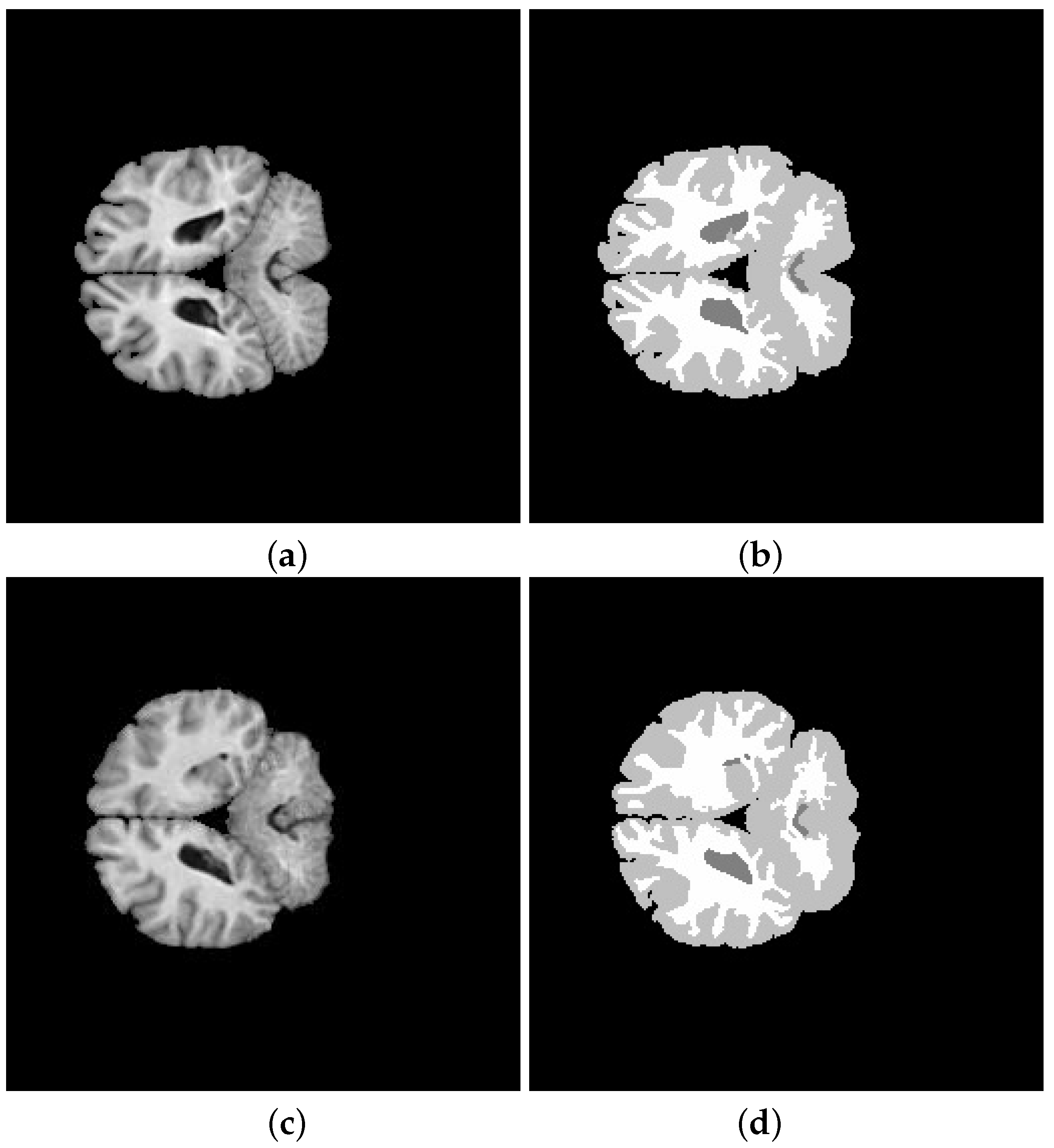
For each subject, we extracted three slices, hence we considered a total of 60 images for segmentation. We used 80% of images to assess the parameters of each clustering method and the remaining 20% for the final test using the best parameter setting found for each method. Figure 3 shows two examples of test images used in the experiments and their corresponding ground truth segmentation.
The gray values of the pixels in the brain image were taken as the basis for clustering. Each clustering algorithm was executed for different parameter settings. In Table 1, we show the parameter values considered for each algorithm. The number of clusters K was varied from 4 to 10. For the fuzziness parameter m, we considered the values . For the SFCM algorithm, we considered all combinations of the values , and . For the application of the KFCM algorithm, a window size () equal to 1, 3 and 5 was considered. Furthermore, we considered different filtering options () i.e., average, median and weighted.
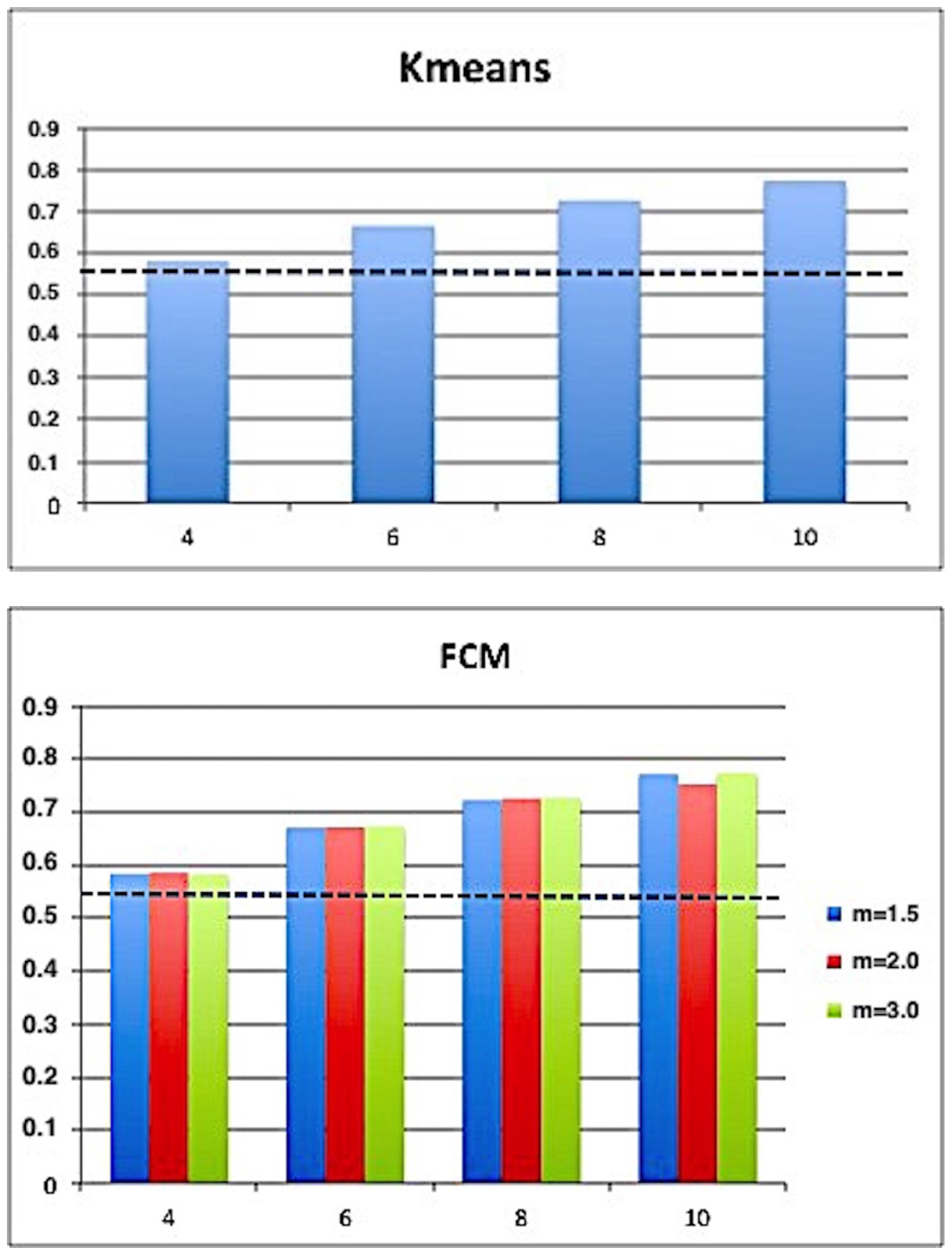
In order to assess and compare the segmentation results obtained by the considered clustering methods, we used the entropy-based evaluation measure E described in Section 4. The measure was evaluated for each clustering algorithm, by varying the number of clusters and the other parameters. Figure 4 plots the values of E averaged on all 48 images for all the considered algorithms with different combinations of parameters. It can be seen that in each case, the optimal number of clusters is . This is compatible with the task of segmenting the brain image into three tissue regions (GM, WM, CSF) plus the background region. In Table 2, we summarize the average values of the E-measure with the standard deviation obtained on the test images. To better compare the methods, we applied a z-test to test the hypothesis that a method outperforms other methods. We found that the null hypothesis can be rejected for SFCM with the smallest p-value (confidence level); hence, we can conclude that SFCM outperforms the other methods.
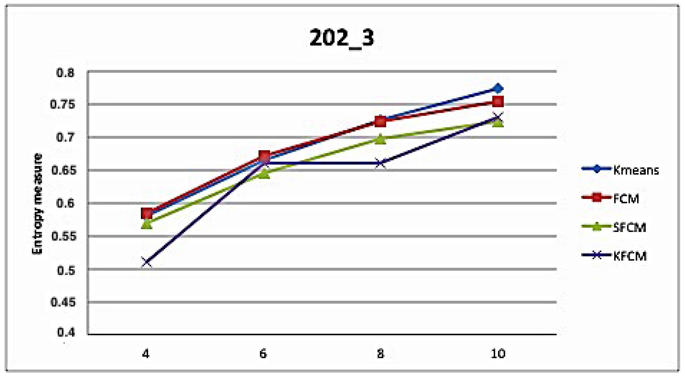
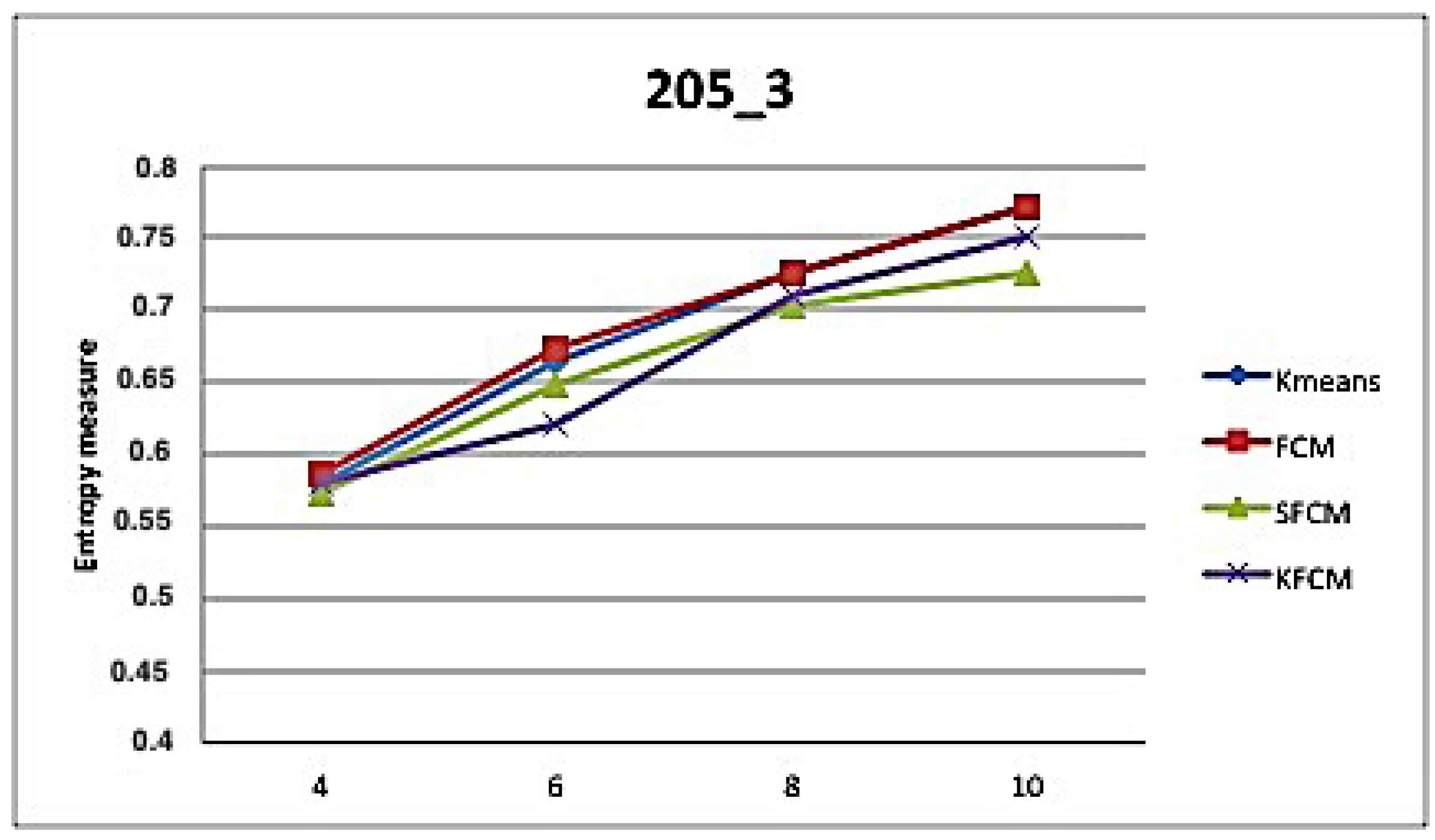
Figure 5 plots the best values of E in the case of segmentation of the two images shown in Figure 3 using the optimal parameter setting. For all algorithms, the optimal configuration includes and . For SFCM, the optimal values for the remaining parameters are , and . Finally, the KFCM provides better results with window size and . It is interesting to note that the same optimal configuration has been found for most of the images.
Besides the E measure, we considered the other evaluation measures described in Section 4 to assess and compare the results. In Table 3, we compare the performance of the considered algorithms in terms of these measures, by averaging over all the classes. For each algorithm, the optimal parameter setting is considered. We found that SFCM provides better results even in terms of these evaluation metrics.
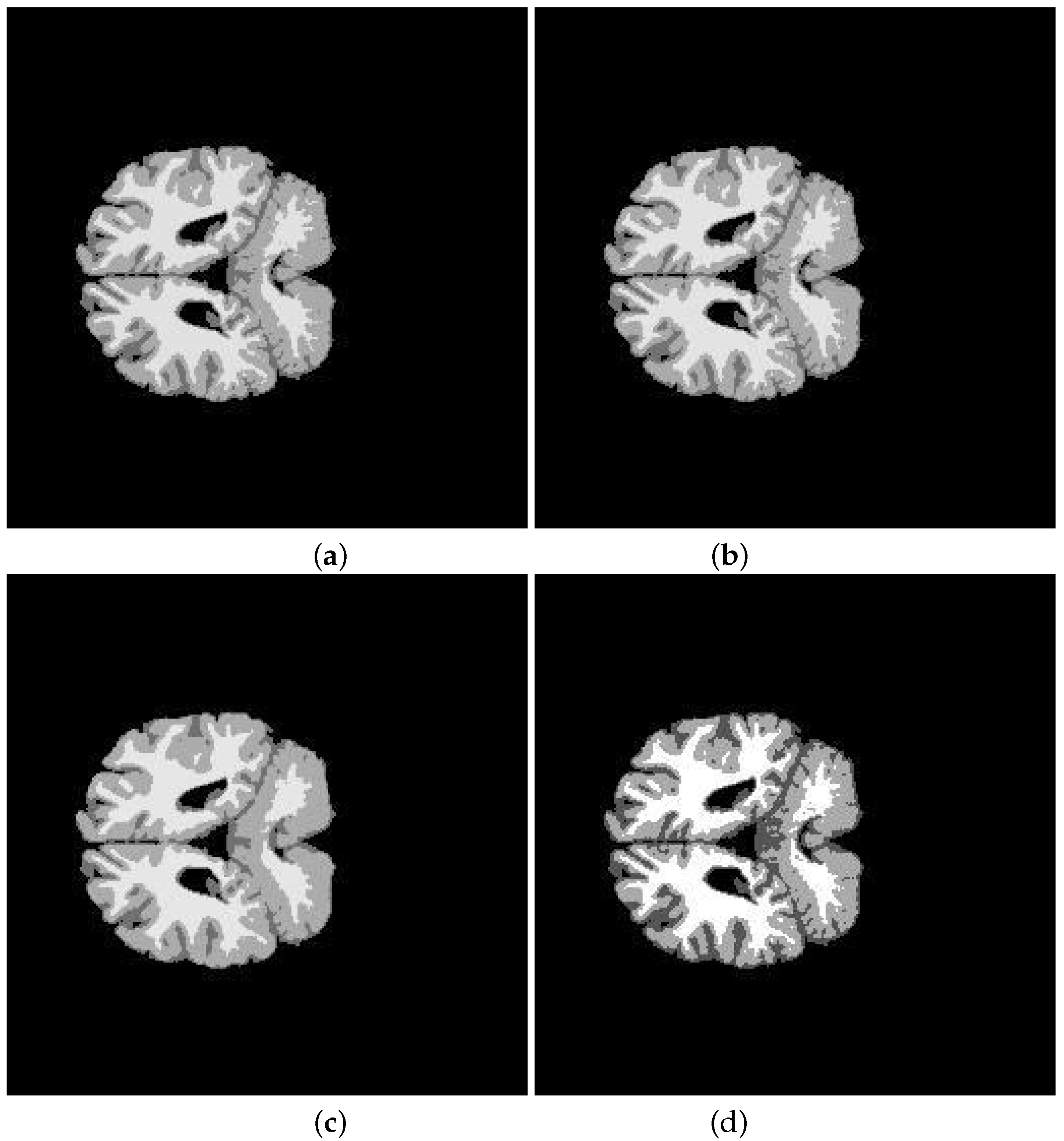
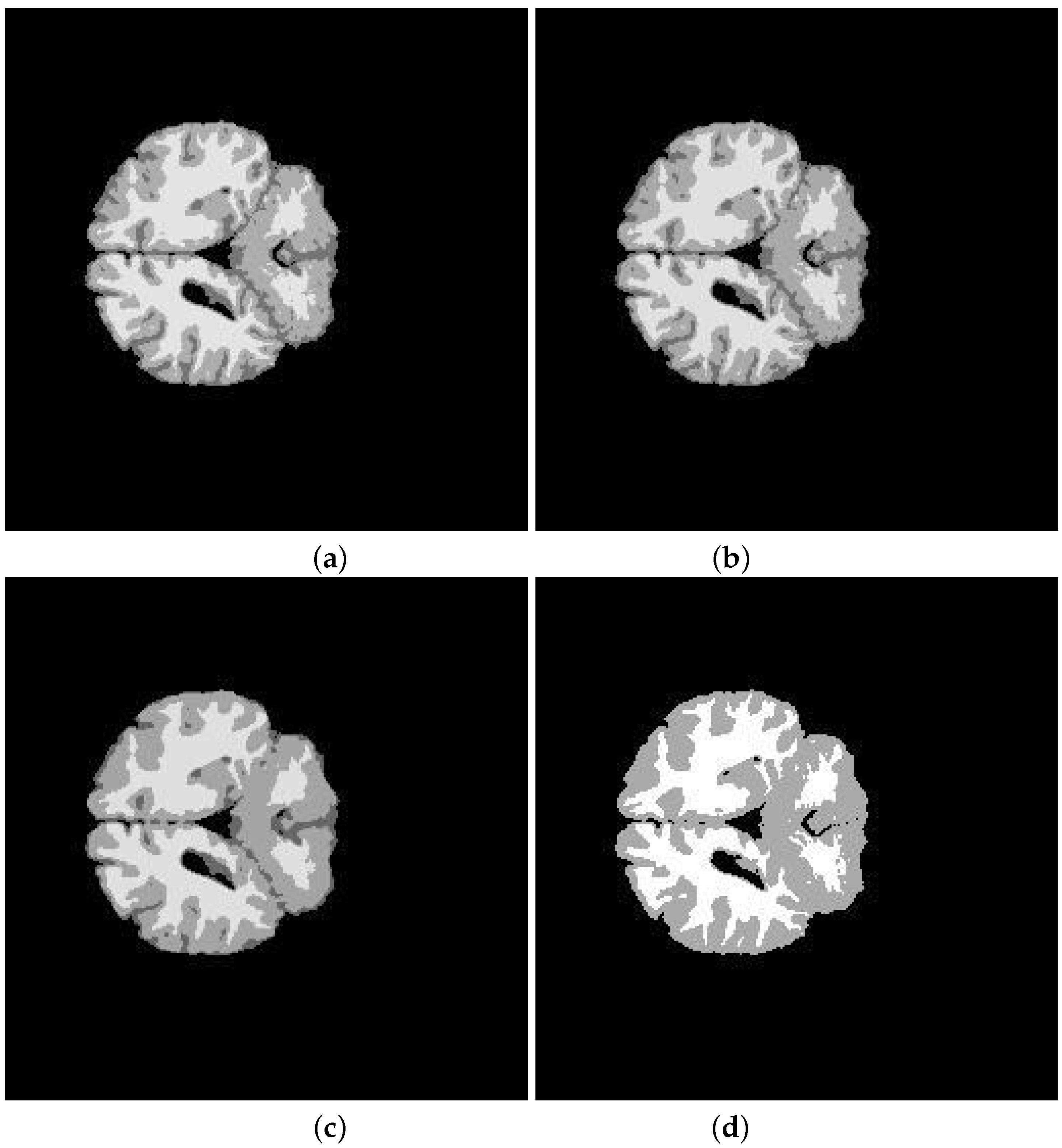
Figure 6 and Figure 7 show the segmented MR brain image using K-means, FCM, spatial FCM and kernelized FCM, respectively. By observing the values of the performance measures, as well as the segmented images, we can conclude that SFCM can segment the brain images better than the other methods. Moreover, it is interesting to note that, despite the segmented images looking quite similar to the original images, the value of the entropy-based measure computed on the original images is about , hence much higher than the values obtained on the segmented images.
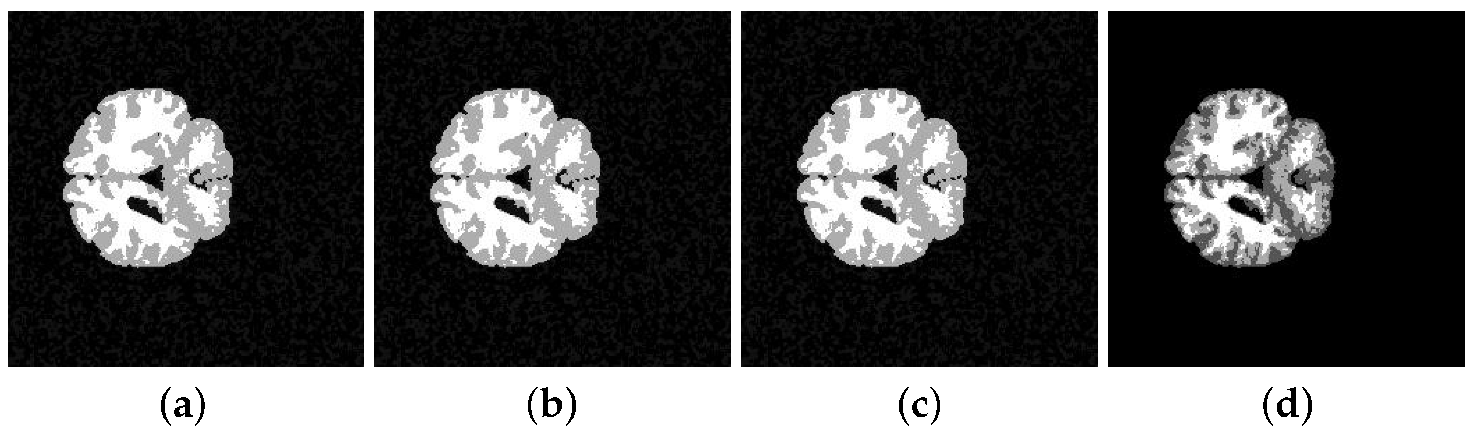
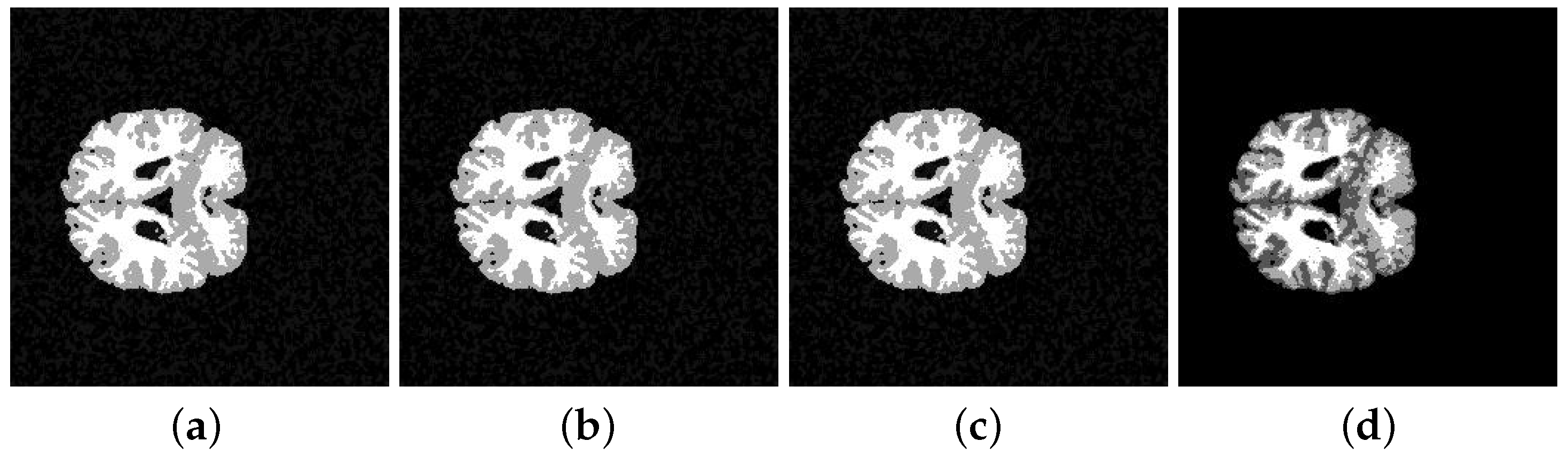
Finally, we tested the sensitivity of the algorithms in the presence of noise. To this aim, all test images were corrupted by 10% salt and pepper noise, and then, a simple median filter was applied to minimize the noise before applying clustering. The median filter is a non-linear filter that preserves edges while removing impulsive noise (outliers). It consists of replacing each center pixel of an neighborhood window with the median of the neighborhood window pixels. In this work, a window size is used. Figure 8 shows two test images corrupted by noise. The segmentation results obtained on these two noisy images are shown qualitatively in Figure 9 and Figure 10. Quantitative results are shown in Table 4 where a comparison with segmentation results on the original images is also given. Even in presence of noise, the SFCM algorithm succeeds in achieving better clustering results.
A final step in medical image segmentation is labeling. Labeling is the process of assigning a meaningful designation to each region obtained by clustering and can be performed separately from segmentation. It maps the numerical index j of region to an anatomical designation. In our medical application, the labels (GM, WM, CSF) can be assigned upon inspection by a physician or technician. Hence, the clustered images should be further analyzed for a final classification of all regions.
6. Conclusions
The segmentation of brain MR images is an important, but challenging step in medical image analysis in both clinical and research areas. Various techniques, such as threshold-based, clustering-based or hybrid methods, have been developed and optimized to perform brain image segmentation. However, not all techniques produce a high accuracy rate. In this paper, we have proposed a framework for image segmentation that includes several clustering algorithms. Using the framework, we showed that clustering algorithms are effective methods for brain image segmentation. In particular, clustering embedded with spatial information succeeds in segmenting the MR images very well. The developed framework offers both qualitative and quantitative evaluation of the segmentation results; hence, it represents a valid support to the analysis of brain images. Further work is addressed to extend the framework so as to include the possibility to combine various clustering methods in order to achieve more robust segmentation results.
Author Contributions
L. Caponetti and G. Castellano conceived and designed the experiments; V. Corsini analyzed the data and performed the experiments; L. Caponetti and G. Castellano wrote the paper.
Conflicts of Interest
The authors declare no conflict of interest.
References
- Wells, W.M.; Grimson, W.E.L.; Kikinis, R.; Jolesz, F.A. Adaptive segmentation of MRI data. IEEE Trans. Med. Imaging 1996, 15, 429–442. [Google Scholar] [CrossRef] [PubMed]
- Forouzanfar, M.; Forghani, N.; Teshnehlab, M. Parameter optimization of improved fuzzy c-means clustering algorithm for brain MR image segmentation. Eng. Appl. Artif. Intell. 2010, 23, 160–168. [Google Scholar] [CrossRef]
- Counsell, S.J.; Boardman, J.P. Differential brain growth in the infant born preterm: Current knowledge and future developments from brain imaging. Sem. Fetal Neonatal Med. 2005, 10, 403–410. [Google Scholar] [CrossRef] [PubMed]
- Nishida, M.; Makris, N.; Kennedy, D.N.; Vangel, M.; Fischl, B.; Krishnamoorthy, K.S.; Caviness, V.S.; Grant, P.E. Detailed semiautomated MRI based morphometry of the neonatal brain: Preliminary results. Neuroimage 2006, 32, 1041–1049. [Google Scholar] [CrossRef] [PubMed]
- Cordato, N.J.; Duggins, A.J.; Halliday, G.M.; Morris, J.G.; Pantelis, C. Clinical deficits correlate with regional cerebral atrophy in progressive supranuclear palsy. Brain 2005, 128, 1259–1266. [Google Scholar] [CrossRef] [PubMed]
- Sepulcre, J.; Sastre-Garriga, J.; Cercignani, M.; Ingle, G.T.; Miller, D.H.; Thompson, A.J. Regional gray matter atrophy in early primary progressive multiple sclerosis: A voxel-based morphometry study. Arch. Neurol. 2006, 8, 1175–1180. [Google Scholar] [CrossRef] [PubMed]
- Fotenos, A.F.; Snyder, A.Z.; Girton, L.E.; Morris, J.C.; Buckner, R.L. Normative estimates of cross-sectional and longitudinal brain volume decline in aging and AD. Neurology 2005, 64, 1032–1039. [Google Scholar] [CrossRef] [PubMed]
- Ridha, B.H.; Barnes, J.; Bartlett, J.W.; Godbolt, A.; Pepple, T.; Rossor, M.N.; Fox, N.C. Tracking atrophy progression in familial Alzheimer’s disease: A serial MRI study. Lanc. Neurol. 2006, 5, 828–834. [Google Scholar] [CrossRef]
- Meyer-Lindenberg, A.; Mervis, C.B.; Sarpal, D.; Koch, P.; Steele, S.; Kohn, P.; Marenco, S.; Morris, C.A.; Das, S.; Kippenhan, S.; et al. Functional, structural, and metabolic abnormalities of the hippocampal formation in Williams syndrome. J. Clin. Investig. 2005, 115, 1888–1895. [Google Scholar] [CrossRef] [PubMed]
- Ciumas, C.; Savic, I. Structural changes in patients with primary generalized tonic and clonic seizures. Neurology 2006, 67, 683–686. [Google Scholar] [CrossRef] [PubMed]
- Henriksson, K.M.; Wickstrom, K.; Maltesson, N.; Ericsson, A.; Karlsson, J.; Lindgren, F.; Astrom, K.; McNeil, T.F.; Agartz, I. A pilot study of facial, cranial and brain MRI morphometry in men with schizophrenia. Psychiatr. Res. Neuroimaging 2006, 147, 187–195. [Google Scholar] [CrossRef] [PubMed]
- Honea, R.; Crow, T.J.; Passingham, D.; Mackay, C.E. Regional deficits in brain volume in schizophrenia: A meta-analysis of voxel-based morphometry studies. Am. J. Psychiatr. 2005, 162, 2233–2245. [Google Scholar] [CrossRef] [PubMed]
- Lim, K.O.; Pfefferbaum, A. Segmentation of MR brain images into cerebrospinal fluid spaces, white and gray matter. J. Comput. Assist. Tomogr. 1989, 13, 588–593. [Google Scholar] [CrossRef] [PubMed]
- Suzuki, H.; Toriwaki, J. Automatic segmentation of head MRI images by knowledge guided thresholding. Comput. Med. Imaging Graph. 1991, 15, 233–240. [Google Scholar] [CrossRef]
- Canny, J.A. A computational approach to edge detection. IEEE Trans. Pattern Anal. Mach. Intell. 1986, 6, 679–698. [Google Scholar] [CrossRef]
- Pohle, R.; Toennies, K.D. Segmentation of medical images using adaptive region growing. In Proceedings of the International Society for Optics and Photonics (SPIE), San Diego, CA, USA, 3 July 2001; p. 4322. [Google Scholar] [CrossRef]
- Li, C.; Huang, R.; Ding, Z.; Gatenby, J.C.; Metaxas, D.N.; Gore, J.C. A level set method for image segmentation in the presence of intensity inhomogeneities with application to MRI. IEEE Trans. Image Process. 2011, 20, 2007–2016. [Google Scholar] [PubMed]
- Ciecholewski, M. An edge-based active contour model using an inflation/deflation force with a damping coefficient. Expert Syst. Appl. 2016, 44, 22–36. [Google Scholar] [CrossRef]
- Zhang, K.; Song, H.; Zhang, L. Active contours driven by local image fitting energy. Pattern Recognit. 2010, 43, 1199–1206. [Google Scholar] [CrossRef]
- Dhanachandra, N.; Chanu, Y.J. A Survey on Image Segmentation Methods using Clustering Techniques. Eur. J. Eng. Res. Sci. 2017, 2, 15–20. [Google Scholar] [CrossRef]
- Jain, A.K.; Dubes, R.C. Algorithms for Clustering Data; Prentice Hall: Englewood Cliffs, NJ, USA, 1988. [Google Scholar]
- Li, C.L.; Goldgof, D.B.; Hall, L.O. Knowledge-based classification and tissue labeling of MR images of human brain. IEEE Trans. Med. Imaging 1993, 12, 740–750. [Google Scholar] [CrossRef] [PubMed]
- Agrawal, S.; Panda, R.; Dora, L. A study on fuzzy clustering for magnetic resonance brain image segmentation using soft computing approaches. Appl. Soft Comput. 2014, 24, 522–533. [Google Scholar] [CrossRef]
- Bezdek, J.C. Pattern Recognition with Fuzzy Objective Function Algorithms; Kluwer Academic Publishers: New York, NY, USA, 1981. [Google Scholar]
- Patel, B.C.; Sinha, G.R. An adaptive k-means clustering algorithm for breast image segmentation. Int. J. Comput. Appl. 2010, 10, 35–38. [Google Scholar] [CrossRef]
- Chen, W.; Giger, M.L.; Bick, U. A fuzzy c-means (FCM)-based approach for computerized segmentation of breast lesions in dynamic contrast-enhanced MR images. Acad. Radiol. 2006, 13, 63–72. [Google Scholar] [CrossRef] [PubMed]
- Ghane, N.; Vard, A.; Talebi, A.; Nematollahy, P. Segmentation of White Blood Cells From Microscopic Images Using a Novel Combination of K-Means Clustering and Modified Watershed Algorithm. J. Med. Signals Sens. 2017, 7, 92–101. [Google Scholar] [PubMed]
- Karthikeyan, T.; Poornima, N. Microscopic Image Segmentation Using Fuzzy C Means for Leukemia Diagnosis. Leukemia 2017, 4, 3136–3142. [Google Scholar]
- Kechagias-Stamatis, O.; Aouf, N.; Nam, D.; Belloni, C. Automatic X-ray Image Segmentation and Clustering for Threat Detection. In Target and Background Signatures III, 104320O; SPIE: Bellingham, WA, USA, 2017. [Google Scholar] [CrossRef]
- Son, L.H.; Tuan, T.M. Dental segmentation from X-ray images using semi-supervised fuzzy clustering with spatial constraints. Eng. Appl. Artif. Intell. 2017, 59, 186–195. [Google Scholar] [CrossRef]
- Ji, Z.; Liu, J.; Cao, G.; Sun, Q.; Chen, Q. Robust spatially constrained fuzzy c-means algorithm for brain MR image segmentation. Pattern Recognit. 2014, 47, 2454–2466. [Google Scholar] [CrossRef]
- Portela, N.M.; Cavalcanti, G.D.C.; Ren, T.I. Semi-supervised clustering for MR brain image segmentation. Expert Syst. Appl. 2014, 41, 1492–1497. [Google Scholar] [CrossRef]
- Zhang, Y.; Ye, S.; Ding, W. Based on rough set and fuzzy clustering of MRI brain segmentation. Int. J. Biomath. 2017, 10, 1750026. [Google Scholar] [CrossRef]
- Kaya, I.E.; Pehlivanlı, A.Ç.; Sekizkardeş, E.G.; Ibrikci, T. PCA based clustering for brain tumor segmentation of T1w MRI images. Comput. Methods Progr. Biomed. 2017, 140, 19–28. [Google Scholar] [CrossRef] [PubMed]
- Novelli, A.; Aguilar, M.A.; Aguilar, F.J.; Nemmaoui, A.; Tarantino, E. AssesSeg—A Command Line Tool to Quantify Image Segmentation Quality: A Test Carried Out in Southern Spain from Satellite Imagery. Remote Sens. 2017, 9, 40. [Google Scholar] [CrossRef]
- Neubert, M.; Herold, H.; Meinel, G. Evaluation of Remote Sensing Image Segmentation Quality–Further Results and Concepts. Available online: http://www.isprs.org/proceedings/xxxvi/4-c42/papers/10_Adaption%20and%20further%20development%20II/OBIA2006_Neubert_Herold_Meinel.pdf (accessed on 4 November 2017).
- Keshavan, A.; Datta, E.; McDonough, I.M.; Madan, C.R.; Jordan, K.; Henry, R.G. Mindcontrol: A web application for brain segmentation quality control. NeuroImage 2017. [Google Scholar] [CrossRef] [PubMed]
- Udupa, J.K.; LeBlanc, V.R.; Zhuge, Y.; Imielinska, C.; Schmidt, H.; Currie, L.M.; Hirsch, B.E.; Woodburn, J. A framework for evaluating image segmentation algorithms. Comput. Med. Imaging Gr. 2006, 30, 75–87. [Google Scholar] [CrossRef] [PubMed]
- Zhang, H.; Fritts, J.E.; Goldman, S.A. An entropy-based objective evaluation method for image segmentation. In Electronic Imaging; International Society for Optics and Photonics: Bellingham, WA, USA, 2004; pp. 38–49. [Google Scholar] [CrossRef]
- Haralick, R.M.; Shapiro, L.G. Image segmentation techniques. Comput. Vision Gr. Image Proc. 1985, 29, 100–132. [Google Scholar] [CrossRef]
- Gonzalez, R.C.; Woods, R.E. Digital Image Processing; Addison-Wesley: Reading, MA, USA, 1992. [Google Scholar]
- Pal, N.R.; Pal, S.K. A review on image segmentation techniques. Pattern Recognit. 1993, 26, 1277–1294. [Google Scholar] [CrossRef]
- Langan, D.A.; Modestino, J.W.; Zhang, J. Cluster validation for unsupervised stochastic model-based image segmentation. IEEE Trans. Image Proc. 1998, 7, 180–195. [Google Scholar] [CrossRef] [PubMed]
- MacQueen, J.B. Some Methods for classification and analysis of multivariate observations. In Proceedings of the 5-th Berkeley Symposium on Mathematical Statistics and Probability; Le Cam, L.M., Neyman, J., Eds.; University of California Press: Berkeley, CA, USA, 1967; pp. 281–297. [Google Scholar]
- Bezdek, J.C.; Hall, L.; Clarke, L. Review of MR image segmentation using pattern recognition. Med. Phys. 1993, 20, 1033–1048. [Google Scholar] [CrossRef] [PubMed]
- Udupa, J.K.; Wei, L.; Samarasekera, S.; Miki, Y.; Van Buchem, M.A.; Grossman, R.I. Multiple sclerosis lesion quantification using fuzzy-connectedness principles. IEEE Trans. Med. Imaging 1997, 16, 598–609. [Google Scholar] [CrossRef] [PubMed]
- Masoole, M.G.; Moosavi, A.S. An improved fuzzy algorithm for image segmentation. World Acad. Sci. Eng. Technol. 2008, 38, 400–404. [Google Scholar]
- Shen, S.; Sandham, W.; Granat, M.; Sterr, A. MRI fuzzy segmentation of brain tissue using neighborhood attraction with neural-network optimization. IEEE Trans. Inf. Technol. Biomed. 2005, 9, 459–467. [Google Scholar] [CrossRef]
- Jiang, L.; Wenhui, W. A modified fuzzy c-means algorithm for segmentation of magnetic resonance images. In Proceedings of the VIIth Digital Image Computing: Techniques and Applications, Sydney, Australia, 10–12 December 2003. [Google Scholar]
- Pham, D.L.; Prince, J.L. Adaptive fuzzy segmentation of magnetic resonance images. IEEE Trans. Med. Imaging 1999, 18, 737–752. [Google Scholar] [CrossRef] [PubMed]
- Xu, C.; Pham, D.L.; Prince, J.L. Finding the brain cortex using fuzzy segmentation, isosurfaces, and deformable surfaces. In Information Processing in Medical Imaging. IPMI 1997; Duncan, J., Gindi, G., Eds.; Lecture Notes in Computer Science; Springer: Berlin/Heidelberg, Germany, 1997; Volume 1230, pp. 399–404. [Google Scholar] [CrossRef]
- Kannan, S.R.; Ramathilagam, S.; Sathya, A.; Pandiyarajan, R. Effective fuzzy c-means based kernel function in segmenting medical images. Comput. Biol. Med. 2010, 40, 572–579. [Google Scholar] [CrossRef] [PubMed]
- Alizadeh, S.; Ghazanfari, M.; Fathian, M. Using data mining for learning and clustering FCM. Int. J. Comput. Intell. 2008, 4, 118–125. [Google Scholar]
- Dawant, B.M.; Zijidenbos, A.P.; Margolin, R.A. Correction of intensity variations in MR image for computer-aided tissue classification. IEEE Trans. Med. Imaging 1993, 12, 770–781. [Google Scholar] [CrossRef] [PubMed]
- Johnson, B.; Atkins, M.S.; Mackiewich, B.; Andson, M. Segmentation of multiple sclerosis lesions in intensity corrected multispectral MRI. IEEE Trans. Med. Imaging 1996, 15, 154–169. [Google Scholar] [CrossRef] [PubMed]
- Tolias, Y.A.; Panas, S.M. Image segmentation by a fuzzy clustering algorithm using adaptive spatially constrained membership function. IEEE Trans. Syst. Man Cybern. Part A Syst. Hum. 1998, 28, 359–369. [Google Scholar] [CrossRef]
- Liew, A.W.C.; Leung, S.H.; Lau, W.H. Fuzzy image clustering incorporating spatial continuity. IEEE Proc. Vision Image Signal Proc. 2000, 147, 185–192. [Google Scholar] [CrossRef]
- Chuang, K.S.; Tzeng, H.L.; Chen, S.; Wu, J.; Chen, T.J. Fuzzy c-means clustering with spatial information for image segmentation. Comput. Med. Imaging Gr. 2006, 30, 9–15. [Google Scholar] [CrossRef] [PubMed]
- Caponetti, L.; Castellano, G.; Corsini, V.; Basile, T.M.A. Cytoplasm image segmentation by spatial fuzzy clustering. In Fuzzy Logic and Applications; Fanelli, A.M., Pedrycz, W., Petrosino, A., Eds.; Lecture Notes in Computer Science (LNCS); Springer: New York, NY, USA, 2011; Volume 6857, pp. 253–260. ISBN 978-3-642-23712-6. [Google Scholar] [CrossRef]
- Muller, K.R.; Mika, S.; Ratsch, G.; Tsuda, K.; Scholkopf, B. An Introduction to Kernel-based Learning algorithms. IEEE Trans. Neural Netw. 2001, 12, 181–202. [Google Scholar] [CrossRef] [PubMed]
- Zhang, D.-Q.; Chen, S.-C. A novel kernelized fuzzy C-means algorithm with application in medical image segmentation. Artificial Intell. Med. 2004, 32, 37–50. [Google Scholar] [CrossRef] [PubMed]
- Valverde, S.; Oliver, A.; Cabezas, M.; Roura, E.; Lladò, X. Comparison of 10 brain tissue segmentation methods using revisited ibsr annotations. J. Magn. Reson. Imaging 2015, 41, 93–101. [Google Scholar] [CrossRef] [PubMed]
- Image Plugin Spatial Fuzzy c-Means. Available online: https://sites.google.com/site/cilabuniba/research/sfcm (accessed on 3 November 2017).
- The Internet Brain Segmentation Repository (IBSR). Available online: http://www.cma.mgh.harvard.edu/ibsr/ (accessed on 3 November 2017).
- Kennedy, D.N.; Filipek, P.A.; Caviness, V.S. Anatomic segmentation and volumetric calculations in nuclear magnetic resonance imaging. IEEE Trans. Med. Imaging 1989, 8, 1–7. [Google Scholar] [CrossRef] [PubMed]
Figure 1.
Graphical interface for the selection of Spatial FCM (SFCM) parameters.

Figure 2.
An example of macro in the developed framework.
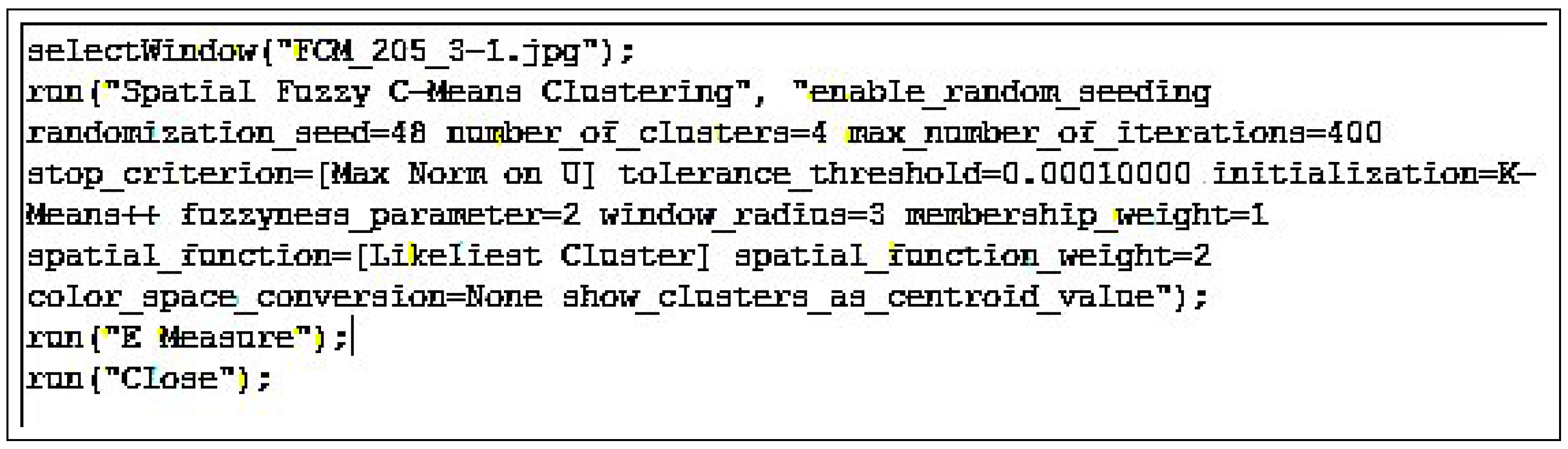
Figure 3.
(a) Original image of Subject 202-3, Slice 20 and (b) its ground truth; (c) original image of Subject 205-3, Slice 20 and (d) its ground truth.
Figure 3.
(a) Original image of Subject 202-3, Slice 20 and (b) its ground truth; (c) original image of Subject 205-3, Slice 20 and (d) its ground truth.

Figure 4.
Average trend of the entropy-based measure. The dotted line refers to the average value computed on the ground truth segmented images.
Figure 4.
Average trend of the entropy-based measure. The dotted line refers to the average value computed on the ground truth segmented images.

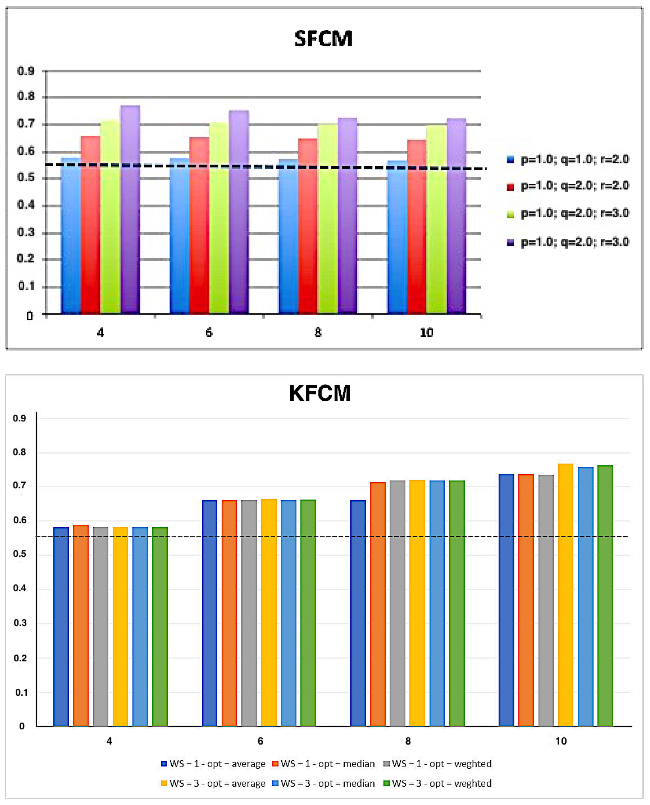
Figure 5.
Entropy-based evaluation measure for the clustering algorithms on Image 202-3 and on Image 205-3 using the optimal parameter setting.
Figure 5.
Entropy-based evaluation measure for the clustering algorithms on Image 202-3 and on Image 205-3 using the optimal parameter setting.


Figure 6.
Best segmentation of Image 202-3 using K-means (a) FCM (b) SFCM (c) and KFCM (d).

Figure 7.
Best segmentation of Image 205-3 using K-means (a) FCM (b) SFCM (c) and KFCM (d).

Figure 8.
The 202-3 (a) and 205-3 (b) images with added noise and the pre-processed images using the median filter (c,d).
Figure 8.
The 202-3 (a) and 205-3 (b) images with added noise and the pre-processed images using the median filter (c,d).
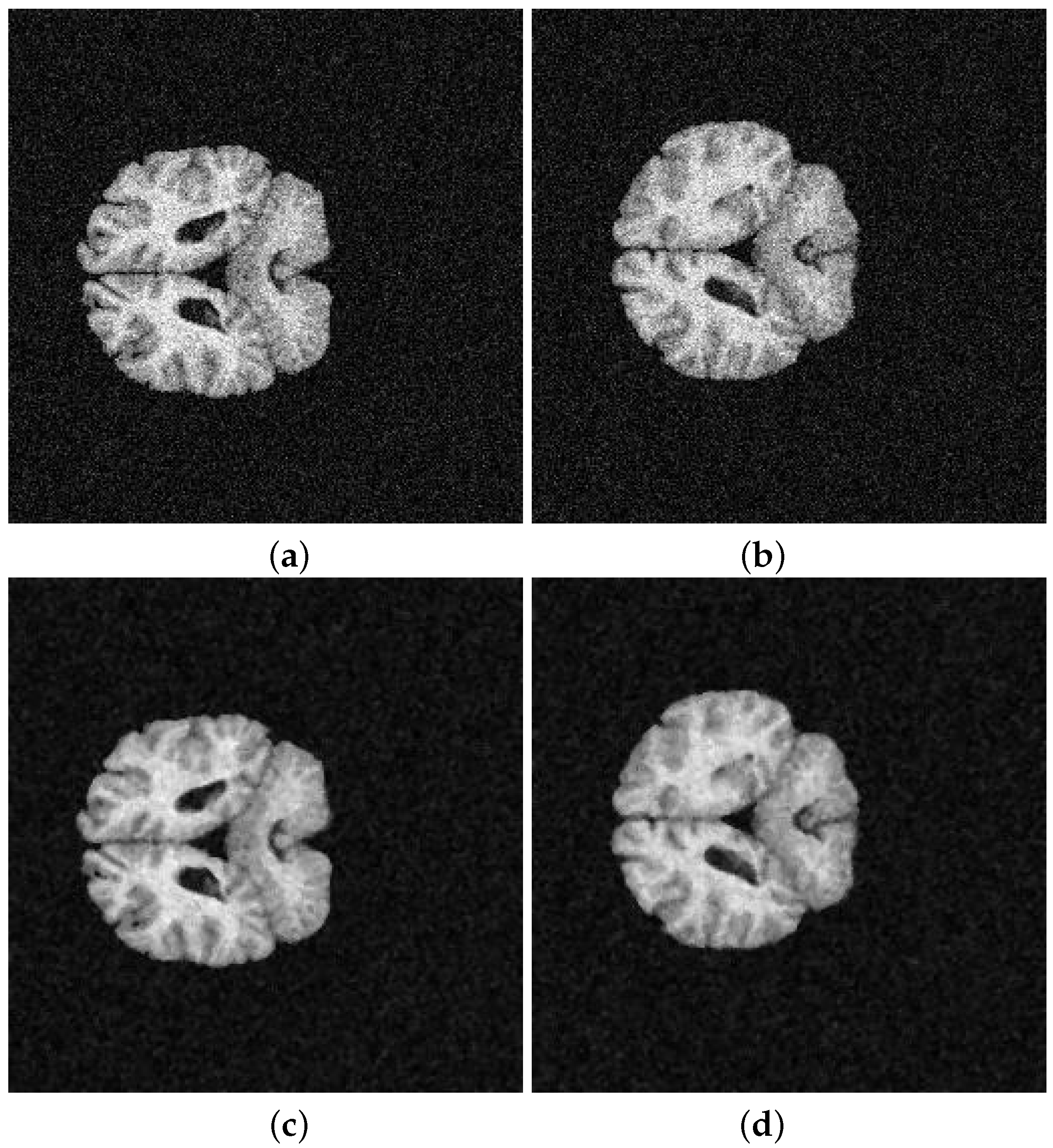
Figure 9.
Segmentation of the noised Image 202-3 using K-means (a) FCM (b) SFCM (c) and KFCM (d).

Figure 10.
Segmentation of the noised Image 205-3 using K-means (a) FCM (b) SFCM (c) and KFCM (d).

Table 1.
Parameters of the clustering algorithms. KFCM, Kernelized FCM.
| K-means | FCM | SFCM | KFCM | |
|---|---|---|---|---|
| K | 4, 6, 8, 10 | 4, 6, 8, 10 | 4, 6, 8, 10 | 4, 6, 8, 10 |
| m | - | 1.0, 1.5, 2.0 | 1.0, 1.5, 2.0 | 1.0, 1.5, 2.0 |
| p | - | - | 1.0, 2.0 | - |
| q | - | - | 1.0, 2.0 | - |
| r | - | - | 2.0, 3.0, 4.0 | - |
| - | - | - | 1, 3, 5 | |
| - | - | - | average, median, weighted |
Table 2.
Average segmentation results obtained by different clustering algorithms on the test images.
Table 2.
Average segmentation results obtained by different clustering algorithms on the test images.
| K-means | FCM | SFCM | KFCM | |
|---|---|---|---|---|
| E-measure | 0.5374 ± 0.0763 | 0.5381 ± 0.0750 | 0.5363 ± 0.0742 | 0.5348 ± 0.0761 |
Table 3.
Comparative results. JS, Jaccard Similarity; DSC, Dice Similarity Coefficient.
| Subject | Method | JS | DSC | Sensitivity | Specificity | Accuracy |
|---|---|---|---|---|---|---|
| K-means | % | |||||
| 202-3 | ||||||
| 0.8938 | 0.9486 | |||||
| K-means | ||||||
| 205-3 | ||||||
Table 4.
Average segmentation results obtained by different clustering algorithms on the test images.
Table 4.
Average segmentation results obtained by different clustering algorithms on the test images.
| Segmented Image | K-means | FCM | SFCM | KFCM |
|---|---|---|---|---|
| 202-3 original | 0.5842 | 0.5850 | 0.5832 | 0.5889 |
| 202-3 with noise | 0.5859 | 0.5873 | 0.5856 | 0.5845 |
| 205-3 original | 0.5793 | 0.5781 | 0.5758 | 0.5761 |
| 205-3 with noise | 0.5763 | 0.5787 | 0.5761 | 0.5782 |
© 2017 by the authors. Licensee MDPI, Basel, Switzerland. This article is an open access article distributed under the terms and conditions of the Creative Commons Attribution (CC BY) license (http://creativecommons.org/licenses/by/4.0/).
Share and Cite
MDPI and ACS Style
Caponetti, L.; Castellano, G.; Corsini, V. MR Brain Image Segmentation: A Framework to Compare Different Clustering Techniques. Information 2017, 8, 138. https://doi.org/10.3390/info8040138
AMA Style
Caponetti L, Castellano G, Corsini V. MR Brain Image Segmentation: A Framework to Compare Different Clustering Techniques. Information. 2017; 8(4):138. https://doi.org/10.3390/info8040138
Chicago/Turabian StyleCaponetti, Laura, Giovanna Castellano, and Vito Corsini. 2017. "MR Brain Image Segmentation: A Framework to Compare Different Clustering Techniques" Information 8, no. 4: 138. https://doi.org/10.3390/info8040138
Note that from the first issue of 2016, this journal uses article numbers instead of page numbers. See further details here.