Histopathological Breast-Image Classification Using Local and Frequency Domains by Convolutional Neural Network


School of Engineering, Macquarie University, Sydney, NSW 2109, Australia
*
Author to whom correspondence should be addressed.
Information 2018, 9(1), 19; https://doi.org/10.3390/info9010019
Submission received: 18 December 2017
/
Revised: 7 January 2018
/
Accepted: 12 January 2018
/
Published: 16 January 2018
(This article belongs to the Special Issue Information-Centered Healthcare)
Abstract
:Identification of the malignancy of tissues from Histopathological images has always been an issue of concern to doctors and radiologists. This task is time-consuming, tedious and moreover very challenging. Success in finding malignancy from Histopathological images primarily depends on long-term experience, though sometimes experts disagree on their decisions. However, Computer Aided Diagnosis (CAD) techniques help the radiologist to give a second opinion that can increase the reliability of the radiologist’s decision. Among the different image analysis techniques, classification of the images has always been a challenging task. Due to the intense complexity of biomedical images, it is always very challenging to provide a reliable decision about an image. The state-of-the-art Convolutional Neural Network (CNN) technique has had great success in natural image classification. Utilizing advanced engineering techniques along with the CNN, in this paper, we have classified a set of Histopathological Breast-Cancer (BC) images utilizing a state-of-the-art CNN model containing a residual block. Conventional CNN operation takes raw images as input and extracts the global features; however, the object oriented local features also contain significant information—for example, the Local Binary Pattern (LBP) represents the effective textural information, Histogram represent the pixel strength distribution, Contourlet Transform (CT) gives much detailed information about the smoothness about the edges, and Discrete Fourier Transform (DFT) derives frequency-domain information from the image. Utilizing these advantages, along with our proposed novel CNN model, we have examined the performance of the novel CNN model as Histopathological image classifier. To do so, we have introduced five cases: (a) Convolutional Neural Network Raw Image (CNN-I); (b) Convolutional Neural Network CT Histogram (CNN-CH); (c) Convolutional Neural Network CT LBP (CNN-CL); (d) Convolutional Neural Network Discrete Fourier Transform (CNN-DF); (e) Convolutional Neural Network Discrete Cosine Transform (CNN-DC). We have performed our experiments on the BreakHis image dataset. The best performance is achieved when we utilize the CNN-CH model on a 200× dataset that provides Accuracy, Sensitivity, False Positive Rate, False Negative Rate, Recall Value, Precision and F-measure of 92.19%, 94.94%, 5.07%, 1.70%, 98.20%, 98.00% and 98.00%, respectively.
1. Introduction
Cancer, being a serious threat to human life, is actually a combination of diseases, and more specifically unwanted and abnormal growth of the cells of the human body is known as cancer. Cancer can attack any part of the body and can then be distributed to any other part. Different types of cancer exist, but, among all the cancers, women are more vulnerable to Breast Cancer (BC) than men because of the anatomical structure of women. Statistics show that each year more people are newly affected by BC, at an alarming rate. Figure 1 shows the number of females newly facing BC as well as the number of females dying since the year 2007 in Australia. This figure shows that more and more females are newly facing BC, and the number of females dying of it has also increased in each year. This is the situation of Australia (population 20–25 million), but it can be used as a symbol of the BC situation of the whole world.
Proper investigation is the first step in proper treatment of any disease. Investigation of BC largely depends on investigation of biomedical images such as Mammograms, Magnetic Resonance Imaging (MRIs) Histopathological, etc. Manual investigation of this kind of images largely depends on the expertise of the doctors and physicians. As humans are error prone, so even an expert can give wrong information about the diagnostic images. Besides this, biomedical image investigation always requires a large amount of time. However, Computer Aided Diagnosis (CAD) techniques are largely utilized for biomedical image analysis such as cancer identification and classification. The use of CAD allows the patient and doctor to take a second opinion.
Different biomedical image analysis techniques are available and different research groups have investigated the identification and classification of BC. The conventional image-classification techniques, such as Support Vector Machines (SVM), Random Forest (RF), Bayesian classifier, etc. algorithms, have been largely utilized for the image classification. Utilizing an SVM, a set of cancer images was first classified by Bazzani et al. and their findings have been compared with the Multi Layer Perception (MLP) technique [1]. Naqa et al. [2] utilized the kernel method along with SVM techniques for better performance for the classification, where they obtained around 93.20% accuracy. A set of Histopathological images has been classified using Scale Invariant Feature Transform (SIFT) and Discrete Cosine Transform (DCT) features with an SVM for classification by Mhala et al. [3]. Law’s Texture features have been utilized for Mammogram (322 images) image classification and 86.10% accuracy obtained by Dheeba et al. [4]. Taheri et al. [5] utilized intensity information, Auto Correlation Matrix and Energy values for breast-image classification and obtained 96.80% precision and 92.50% recall with 600 Mammogram images. A set of ultrasound images have been classified by Shirazi et al. [6], where Regions of Interest (ROI) have been extracted for reduction of the computational complexity. Levman et al. [7] classify a set of MRI images (76 images) into benign and malignant classes, utilizing Relative Signal Intensities and Derivative of Signal Strength as features.
The RF method has also been used for image classification. A set of Mammogram images has been classified by Angayarkanni et al. [8], and they achieved 99.50% accuracy using the Gray-Level-Cooccurence Matrix (GLCM) as feature. Gatuha et al. [9] utilized Mammogram images for image classification using a total of 11 features and achieved 97.30% accuracy. Breast Histopathological images have been classified by Zhang et al. [10] and they achieved 95.22% accuracy, where they utilized the Curvelet Transform, GLCM, and Completed Local Binary Pattern (CLBP) methods for feature extraction. GLCM and Gray-Level-Run-Length-Matrix (GLRLM) have been utilized along with the RF algorithm by Diz et al. [11] for Mammogram image classification with 76.60% accuracy. The Bayes method has also been used for image classification. Kendall et al. [12] utilized the Bayes method for Mammogram image classification with the DCT method for feature selection. Their obtained sensitivity was 100.00% and specificity was 64%. Statistical and Local Binary Pattern (LBP) features along with the Bayesian method have been utilized by Claridge et al. [13] on two Mammogram image sets. When they used the Mammographic Image Analysis Society (MIAS) dataset, their best achieved accuracy was 62.86%.
Other than RF, SVM, Bayes method, and the Neural Network (NN) method have largely been utilized for image classification. Rajakeerthana et al. [14] classified a set of Mammogram images and obtained 99.20% accuracy. Thermographic images have been classified by Lessa et al. [15], and they utilized the NN method along with a few statistical values such as mean, median, skewness, kurtosis, median as features and obtained 85.00% accuracy with a specificity value of 83.00%. Harlick and Tamura features have been utilized by Peng et al. [16] along with an NN network. They used Rough-Set theory for the feature reduction. Silva et al. [17] utilized 22 different morphological features such as convexity, lobulation index, elliptic normalized skeleton along with NN for ultrasound image classification and obtained 96.98% accuracy. Melendez et al. [18] utilized Area, Perimeter, Circularity, Solidity, etc. along with NN and achieved sensitivity and specificity of 96.29% and 99.00%.
As the literature shows, different methods and techniques have been utilized for image classification on different breast-image datasets using different image-classification techniques. However, the state-of-the-art image classification technique of the Convolutional Neural Network (CNN) has put its strong footprint in the image-analysis field, especially the image-classification field. Though the model “AlexNet” proposed by Krizhevsky has gained a new momentum in the CNN research field, a CNN model was first utilized by Fukushima et al. [19] who proposed the “Necognitron” model that recognises stimulus patterns. For the mammogram image classification, Wu et al. first utilized the CNN model [20]. Though little work on the CNN model had been done to the end of the 20th century, this model has only gained momentum from the AlexNet model. Advanced engineering techniques have been used by research groups such as the Visual Geometry Group and Google, which have modeled the VGG-16, VGG-19 and GoogleNet models. Arevalo et al. [21] classified benign and malignant lesions using the CNN model, and this experiment was performed on 766 mammogram images, where 426 images contain benign and 310 malignant lesions. Before classifying the data, they utilized preprocessing techniques to increase the image enhancement and obtained a 0.82 ± 0.03 Receiver Operating Characteristic (ROC) value. GoogleNet and AlexNet methods have been utilized by Zejmo et al. [22] for the classification of cytological specimens into benign and malignant classes. The best accuracy obtained when they utilized the GoogleNet model was 83.00%. Qiu et al. [23] used the CNN method to extract global features for Mammogram image classification and obtained an average achieved accuracy of 71.40%. Fotin et al. also utilized the CNN method for tomosynthesis image classification and obtained an Area Under the Curve (AUC) value of 0.93. Transfer learning is another important concept of the CNN method that allows the model to not extract features from scratch, rather applying a weight-sharing concept to train a model. This method is helpful when the database contains fewer images. Jiang et al. [24] utilized a transfer learning method for Mammogram image classification and obtained an AUC of 0.88. Before utilizing it in a CNN model, they performed a preprocessing operation to enhance the images. Suzuki et al. [25] also used the benefit of transfer learning techniques to train their model to classify mammogram images and obtained sensitivity 89.9%. They performed their experiment with only 198 images.
Most image classification based on the CNN method has been performed based on global feature-extraction techniques. Recently, researchers have also shown an interest in how local features can be utilized with the CNN model for data classification. Both global and local features have been utilized by Rezaeilouyeh et al. [26] for Histopathological image classification. For local feature extraction, the authors utilized the Shearlet transform and obtained an accuracy of 86 ± 3.00%. For local feature extraction, Sharma et al. [27] used the GLCM, GLDM methods and then fed the local features to a CNN model for the Mammogram image classification, obtaining 75.33% accuracy for the fatty and dense tissue classification. Both global and local features have been used by Jiao et al. [28] for mammogram image classification and they obtained 96.70% accuracy. Kooi et al. [29] utilized both global features and hand-crafted features for Mammogram image classification. In their experiment, they also utilized the transfer learning method.
The Contourlet Transform (CT) has been used for image analysis. Using CT, the distribution of Mammograms (MIAS dataset) has been calculated by Anand et al. [30]. Along with GLCM and morphological features, CT features have been utilized for the Mammogram image classification with the SVM method, and obtained a mean Accuracy around 100.00% by Moayedi et al. [31]. The non-subsampled CT transform has been utilized for Breast mass classification by Leena Jasmine along with the SVM techniques [32]. Pak et al. also utilized Non-subsampled CT for breast-image (MIAS dataset) classification and obtained 91.43% mean Accuracy and 6.42% mean False Positive Rate (FPR) [33].
Inspired by the usefulness of local-features utilization techniques with the CNN, this paper has also classified a set of Histopathological images (BreakHis dataset) using local features along with the CNN model. For the local-feature selection, we have utilized the CT transform, LBP and Histogram information. We have also extracted frequency-domain information and tried to find how the CNN model behaves when we provide frequency-domain information. To do so, we have organized our paper as follows: Section 1 describes related research, Section 2 describes the overall architecture for the image classification, Section 3 describes the feature-extraction and data-preparation techniques, Section 4 describes the novel Convolutional-Neural-Network (CNN) model, Section 5 describes the performance measuring parameters, Section 6 describes the performance of our model on the BreakHis dataset as well as compare with the present findings, and we conclude our paper in Section 7.
2. Overall Architecture
Benign and Malignant image classification has always been a challenging task. The level of complication of the data classification increases when we consider Histopathological images, as an example the left side. Figure 2 represents the Benign and the right side figure represent the Malignant images. Every supervised classification technique follows a predefined working mechanism, such as selection of dataset, features and model to perform the classification. Then, a set of performance measuring parameters is tested based on model performance parameters. The selected dataset is normally split into train and test datasets. A hypothetical model is established based on the training dataset, and later this hypothetical model’s performance is evaluated by the test dataset.
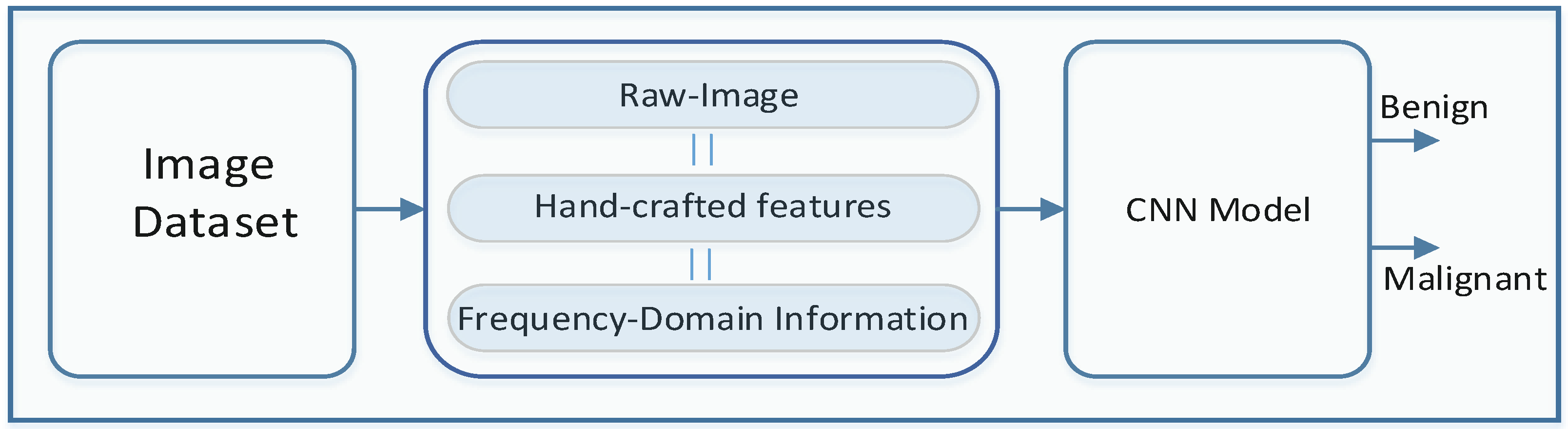
Conventionally, handcrafted features or local features are extracted and utilized for the input of a classifier model. However, in most of the work, using CNN-based image classification, raw images are fed directly to the CNN model. From the raw images, the CNN model tries to extract features globally. In this work, we have utilized raw images as well as descriptive handcrafted local features and frequency-domain information for the image classification along with the CNN model. Figure 3 shows the overall classifier model that has been used for the data classification.
Based on how we prepare the features to feed them in to the CNN model, we have divided our work into the following three cases:
- Case1: In this case, the image has been directly fed to the CNN model, which is named CNN-I. To reduce the complexity, we have reshaped each of the original images of the dataset to a new image matrix of size , where C represents the number of channels. As we have utilized RGB images, the value of .
- Case2: Case2 utilizes local descriptive features that have been collected through the Contourlet Transform (CT), Histogram information and Local Binary Pattern (LBP). Case2 is further divided into two sub cases:
- Case2a: Selected statistical information has been collected from the CT coefficient data and this statistical data has been further concatenated with the Histogram information. This case has been named CNN-CH. The feature matrix for each of the images is represented as .
- Case2b: Selected statistical information has been collected from the CT coefficient data and this statistical data has been further concatenated with the LBP. This case has been named CNN-CL. The feature matrix for each of the images is represented as .
- Case3: Case3 utilizes frequency-domain information for the image classification, collected using the Discrete Fourier Transform (DFT) and the Discrete Cosine Transform (DCT). This case has been further subdivided into two sub-cases:
- Case3a: DFT coefficients have been utilized as an input for the classifier model, named CNN-DF. The feature matrix for each of the images is represented as .
- Case3b: DCT coefficients have been utilized as an input for the classifier model, named CNN-DC. The feature matrix for each of the images is represented as .
3. Feature Extraction and Data Preparation
We have utilized three cases to analyse our data. Case1 or CNN-I directly feeds the raw data to the CNN model for further analysis. However, Case2 and Case3 utilize handcrafted features with CT, Histogram, LBP, Discrete Fourier Transform (DFT) and Discrete Cosine Transform (DCT).
3.1. Data Preparation for Case2
For Case2, we have extracted a set of statistical information utilizing the value of CT coefficients that has been collected after applying CT to each of the images. CT is an extension of the Wavelet Transform (WT). WT ignores the smoothness along the contour and it provides less directional information about the images, whereas CT overcomes this problem of WT and gives better information about the contour and direction edges of an image [34]. CT method utilizes multi-scale Laplacian Pyramid (LP) and a Directional Filter Bank (DFB).
- Laplacian Pyramid (LP): The image pyramid is an image-representation technique where the represented image contains only relatively important information. This technique also produces a series of replications of the original images, but those replicated images have less resolution. A few pyramid methods are available such as Gaussian, Laplacian and WT. Burt and Adelson introduced the Laplacian Pyramid (LP) method. In the case of CT, the LP filter decomposes the input signal into a coarse image and a detailed image (bandpass image) [35]. Each bandpass is further processed and the bandpass directional sub-band signals calculated.
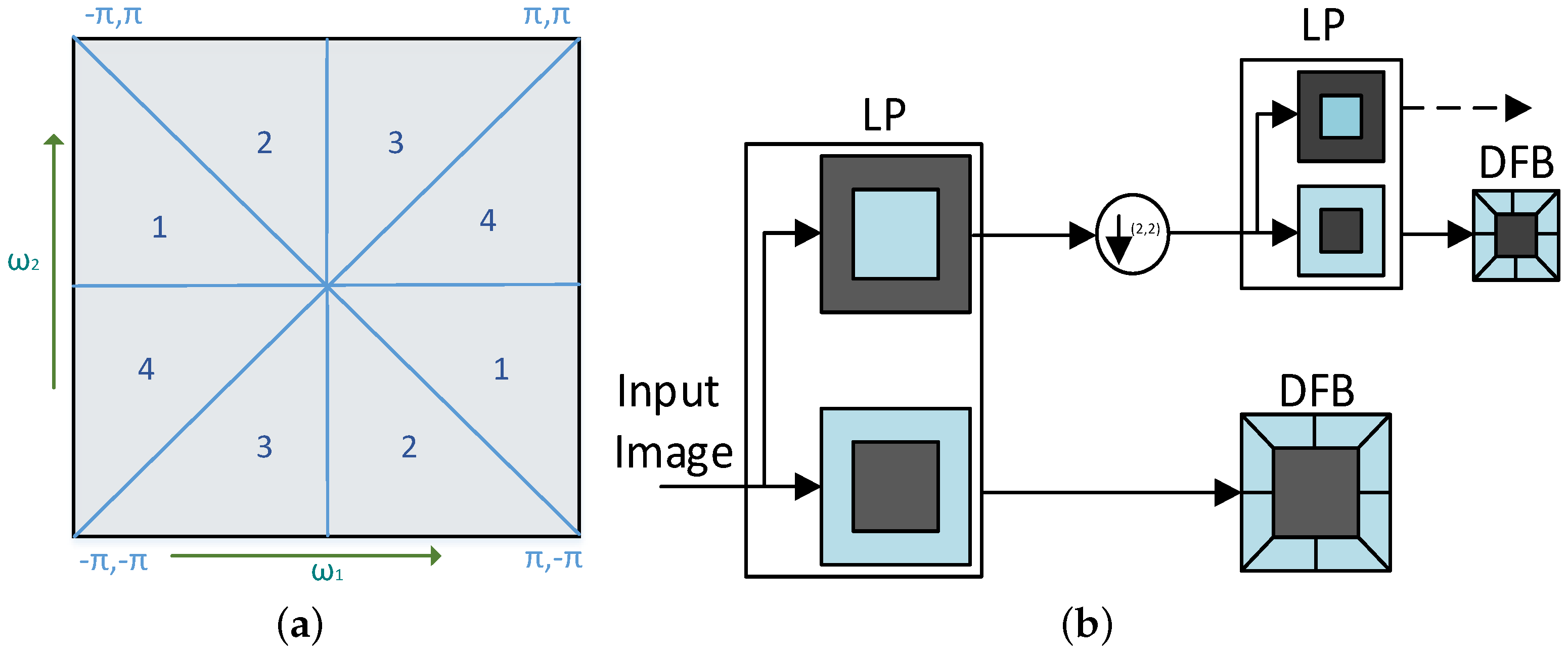
- Directional Filter Bank: A DFB sub-divides the input image into sub-bands. Each of the sub-bands has a wedge-shaped frequency response. Figure 4a shows the wedge-shaped frequency response for a 4-band response.
Let the input image feed to the LP filter (), where , which decomposes images into the low-pass signal and the detailed signal . The detailed image is passed through a DFB to get the directional images. In general, the detailed image at level j, , is further decomposed by DFB into -level directional images . Figure 4b shows an overall CT procedure.
As CT is an iterative operation, it continuously produces low-pass signals and directional signals into some predefined level. Among the available lowpass signals and the directional signals, we have deliberately selected a set (cardinality of the set is sixteen) of statistical features:
- Maximum Value (MA),
- Minimum Value (MI),
- Kurtosis (KU),
- Standard Deviation (ST).
The CT operation has been performed on each of the image channels individually. For a single channel of each of the input images, we calculated sixteen MA, sixteen MI, sixteen KU, and sixteen ST values that have been used as features. Features extracted from the single channel utilizing the CT and statistical method can be written as , so a single channel image produces sixty-four feature values using CT and statistical information. As our images are RGB, we have utilized Red, Green and Blue channels, so the total number of features due to the CT utilization will be .
3.1.1. Histogram Information
A graphical display that represents the frequency of each of the particular intensities in an image is known as a histogram. Let the feature set collected for the histogram information from a single channel be represented as . A single RGB image provides a total features, where the cardinality of will be 768. As Case2a that is CNN-CH utilizes statistical information collected from CT as well as histogram information, the total concatenated features will be , and cardinality of will be 960. We have added zero padding at the end of the feature set to reshape the vector to a matrix, to produce the matrix .
3.1.2. Local Binary Pattern
The Local Binary Pattern (LBP) is proposed by Ojala et al. [36], which represents an image by a two-dimensional matrix, where each entry of this newly created two- dimensional matrix is labeled by an integer. Basically, this matrix represents a local pattern and structural distribution of the image information. A single channel provides 256 LBP features. Let the feature set collected for the LBP information from a single channel be represented as . A single RGB image provides a total features, so the cardinality of will be 768. As Case2b that is CNN-CL utilizes statistical features from CT and LBP, so the total concatenated features will be , with a cardinality of 960. We have added zero padding at the end of the feature set to reshape the vector to a matrix, in order to produce the matrix .
3.2. Data Preparation for Case3
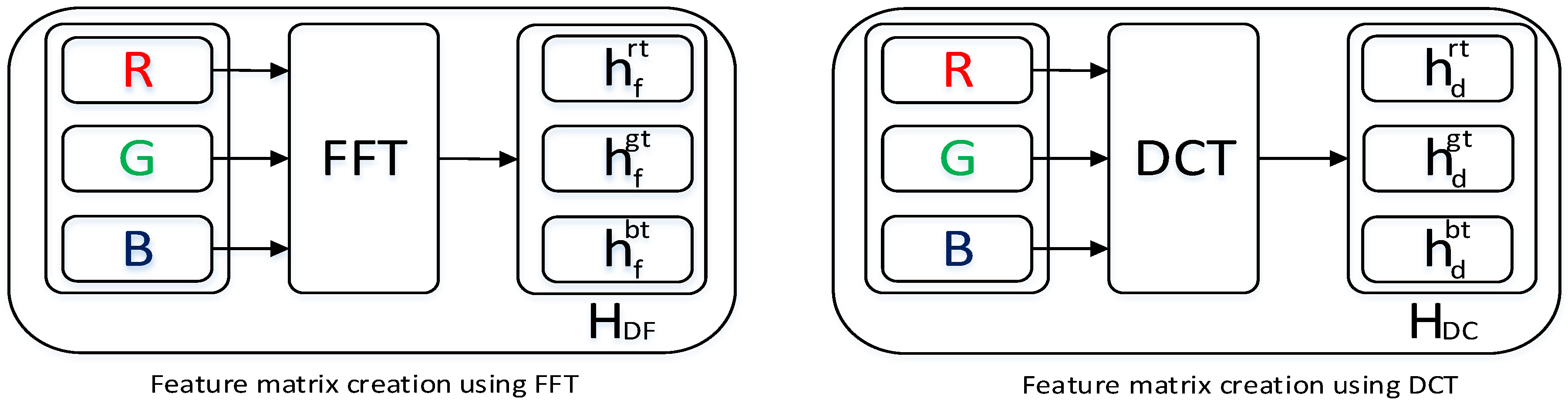
For Case3, we have utilized frequency-domain information as the features. To find the frequency-domain information, we have utilized the DFT and DCT transforms. Figure 5 represents the Feature-Selection procedure for Case3.
3.2.1. DFT for Feature Selection
Frequency-domain information reveals valuable information from the signal which can be extracted using the Fourier Transform. This frequency-domain information can be extracted both from the continuous and discrete-time signal. For the discrete time signal, DFT methods have been utilized for the frequency-domain information extraction. To avoid the computational complexity and timing issues of the DFT, we have utilized the Fast Fourier Transform (FFT) to extract the frequency-domain information. As the Histopathological image contains three channels, the FFT coefficients have been extracted from each of the three channels:
The first top FFT coefficients have been selected from each of the channel where :
Here, represent the feature matrix for the Case3a that is for CNN-DF.
3.2.2. DCT for Feature Selection
Strang first introduced the DCT method in 1974 [37]. A few DCT methods are available, and among them DCT-II methods have been largely utilized for image analysis. As a Histopathological image contains three channels, the DCT coefficients have been extracted from each of the three channels:
The first top “” FFT coefficients have been selected from each of the channels where :
Here, represents the feature matrix for the Case3b that is CNN-DC.
Table 1 summarises extracted local features for different cases:
- Convolutional Neural Network CT Histogram (CNN-CH)
- Convolutional Neural Network CT LBP (CNN-CL)
- Convolutional Neural Network Discrete Fourier Transform (CNN-DF)
- Convolutional Neural Network Discrete Cosine Transform (CNN-DC)
4. Convolutional Neural Network
A CNN model is a state-of-the-art method that has been largely utilized for image processing. A CNN model has the ability to extract global features in a hierarchical manner that ensures local connectivity as well as the weight-sharing property.
- Convolutional Layer: The Convolutional layer is considered as the main working ingredient in a CNN model and plays a vital determining part of this model. A kernel (filter), which is basically an matrix successively goes through all the pixels and extracts the information from them.
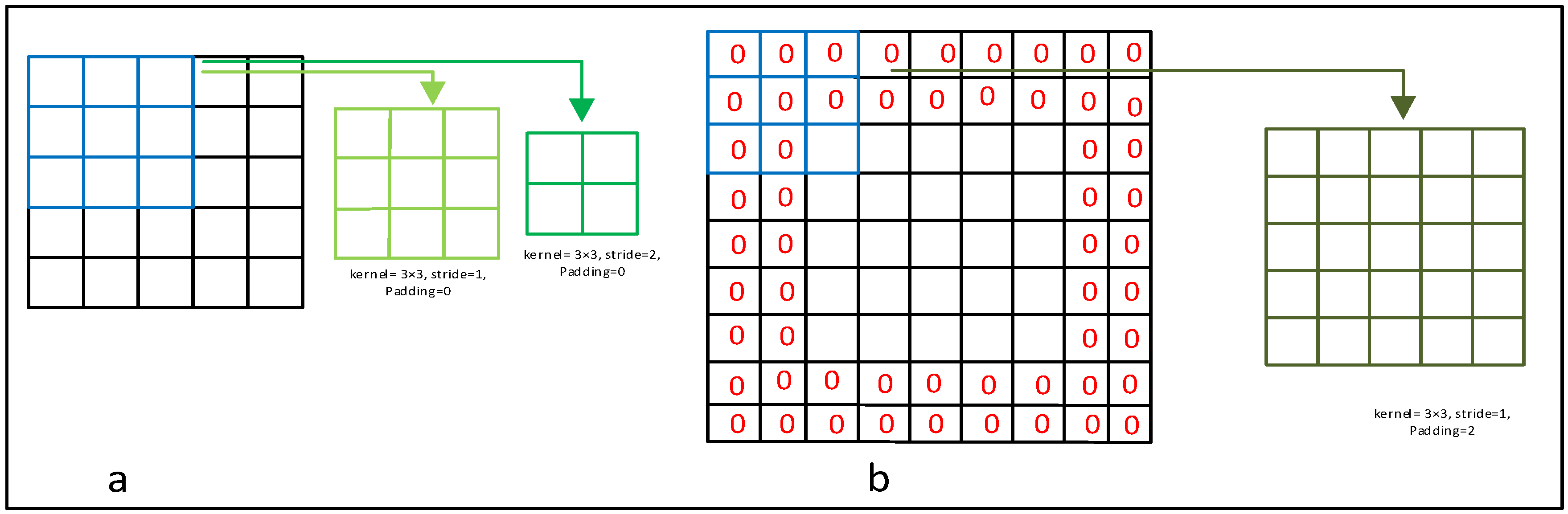
- Stride and Padding: The number of pixels a kernel will move in a step is determined by the stride size; conventionally, the size of the stride keeps to 1. Figure 6a shows an input data matrix of size , which is scanned with a kernel. The light-green image shows the output with stride size 1, and the green image represents the output with stride size 2. When we use a kernel, and stride size 1, then the convolved output is a matrix; however, when we use stride size 2, the convolved output is . Interestingly, if we use a kernel on the above input matrix with stride 1, the output will be a matrix. Thus, the size of the output image has changed with both the size of the stride and the size of the kernel. To overcome this issue, we can utilize extra rows and columns at the end of the matrices that contain 0 s. This adding of rows and columns that contain only zero values is known as zero padding.For example, Figure 6b shows how two extra rows have been added at the top as well as the bottom of the original matrix. Similarly, two extra columns have been added at the beginning as well as the end of the original matrix. Now, the olive-green image of Figure 6b shows a convolved image where we have utilized a kernel of size , stride size 1 and padding size zero. The convolved image is also a matrix, which is the same as the original data size. Thus, by adding the proper amount of zero padding, we can reduce the loss of information that lies at the border.
- Nonlinear Performance: Each layer of the NN produces linear output, and by definition adding two linear functions will also produce another linear output. Due to the linear nature of the output, adding more NN layers will show the same behavior as a single NN layer. To overcome this issue, a rectifier function, such as Rectified Linear Unit (ReLU), Leaky ReLU, TanH, Sigmoid, etc., has been introduced to make the output nonlinear.
- Pooling Operation: A CNN model produces a large amount of feature information. To reduce the feature dimensionality, a down-sampling method named a pooling operation has been performed. A few pooling operation methods are well known such as
- Max Pooling,
- Average Pooling.
For our analysis, we have utilized the Max Pooling operation that selects the maximum values within a particular patch. - Drop-Out: Due to the over training of the model, it shows very poor performance on the test dataset, which is known as over-fitting. These over-fitting issues have been controlled by removing some of the neurons from the network, which is known as Drop-Out.
- Decision Layer: For the classification decision, at the end of a CNN model, a decision layer is introduced. Normally, a Softmax layer or a SVM layer is introduced for this purpose. This layer contains a normalized exponential function and calculates the loss function for the data classification.
Figure 7 shows the work flow of a generalized CNN model that can be used for image classification. Before the decision layer, there must be at least one immediate dense layer available in a CNN model. Utilizing the Softmax layer, the output of the end layer can be represented as
where
Here, represents the kth neuron at the th layer, and represents the nonlinear function. For binary classification, the number of . Let represent the Benign class and else it represents the Malignant class. The cross-entropy loss of can be calculated as
As we are working on a two-class classification problem, then only the and values are possible, and the output will be be when , else the output will be .
CNN Model for Image Classification
For breast-image classification, we have utilized the CNN model with the following architectures:
- Model-1: Model-1 utilizes a residual block, represented as Block-n. Each Block-n contains two convolutional blocks named C-n and R-n. The C-n layer convolves the input data with a kernel along with a ReLU rectifier and produces 16 feature maps. The output of the C-n layer passes through the R-n convolutional layer, which also utilizes a kernel along with a ReLU rectifier. The R-n layer also produces 16 feature maps. The output of the R-n layer is merged with the output of the layer and produces a residual output. The output of Block-n can be represented aswhere represents the weight matrix and represents the bias vector.The input matrix passes through Block-1 and Block-2 as shown in Figure 8 (left image). The Output of Block-1 is fed to Block-3, the output of Block-3 is fed as an input of Block-5, the output of Block-5 is fed as an input of Block-7, and the output of Block-7 is fed as an input of Block-9. Similarly, the output of Block-2 is fed to Block-4, the output of Block-4 is fed as an input of Block-6, the output of Block-6 is fed as an input of Block-8, and the output of Block-8 is fed as an input of the Block-10. Now, the output of Block-9 and Block-10 are concatenated in the Concat layer. After the Concat layer, a Flat Layer, a Drop-Out Layer and a Softmax layer have been placed one after another. The output of the Softmax layer has been used to classify the images into Benign and Malignant classes.
- Model-2: Model-2 utilizes almost the same architecture as Model-1. The only difference is that, in each Block-n, the output of layer C-n is multiplied (rather than added) with the output of layer R-n. The output of Block-n can be represented as
5. Performance Measuring Parameter and Utilized Platform
The performance of a classifier is measured by some basemark criteria, which can be obtained by a two-dimensional matrix known as the Confusion Matrix [38]. The content of the matrix position represents how many times the target is correctly classified. Thus, it is expected that the non-diagonal positions of the Confusion Matrix should be as small as possible. Figure 9 shows a graphical representation of a Confusion Matrix and Table 2 summarizes a few of the well-known classification performance measurement parameters.
Platforms Used
Image pre-processing related tasks are performed in MATLAB (R2016b). Out of the available platforms for CNN model development, we have selected Keras. Lastly, most of the matrix operations are performed on a GeForce GTX 1080 GPU (Taiwan), as the classification of images involves billions of matrix operations, which is not possible with a low-grade CPU.
6. Results and Discussion
For the classification, we utilized the BreakHis data set [39]. The images of this dataset are RGB in nature, having 8-bit depth and a (Portable Network Graphics) PNG extension. The images are pixels in size. All the images are divided into four groups, depending on the visual magnification factor, namely , , and , where × represents the magnification factor. We performed our experiments on the individual groups of the dataset.
6.1. Performance of 40× Dataset
Table 3 shows the performance of Model-1 and Model-2 on the 40× data-set. The overall best performance is achieved when CNN-CH along with Model-1 is utilized. In this situation, the achieved Accuracy is 94.40%, where the Recall and Precision values are 96.00% and 86.00%, respectively. For the Model-1, CNN-CL provides a similar performance. When we use Model-1, the worst Accuracy of 86.47% is achieved when we utilize CNN-DC.
For Model-2, the best Accuracy of 88.31% is achieved when we utilize the CNN-I algorithm. However, the achieved Recall value is 96.00% and the Specificity value is 69.45%, which indicates that almost of the Benign images have been misclassified as Malignant images. When we utilize the CNN-CH algorithm along with Model-2, the Recall value is 100.00% and FPR is 100.00%. This indicates that all the data, irrespective of Benign or Malignant, are classified as Malignant. In terms of Accuracy, CNN-DF and CNN-DC provide a similar performance; however, CNN-DF provides better specificity performance than CNN-DC. More specifically, CNN-DC mis-classifies almost 50.00% of the Benign data as Malignant data.
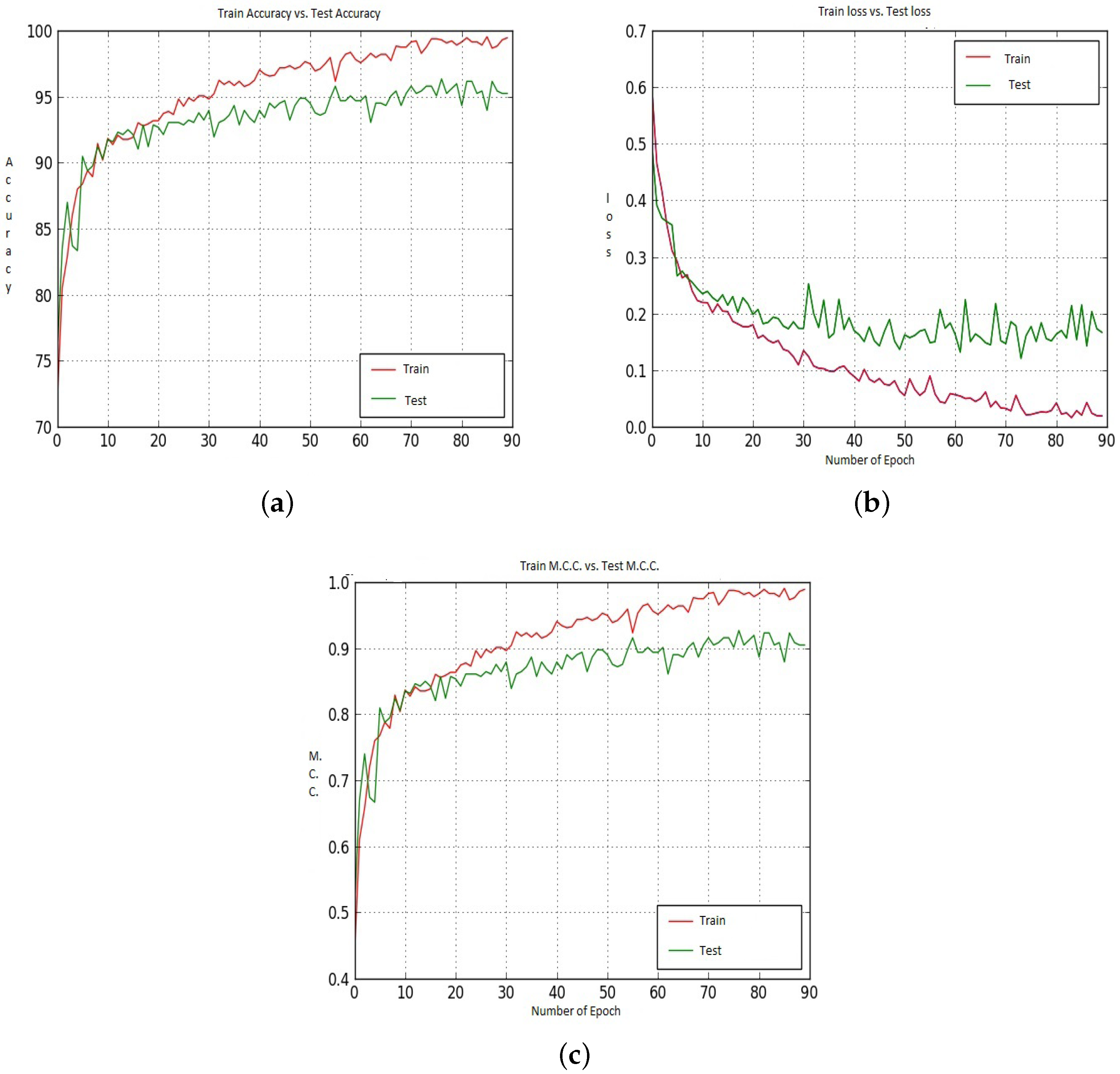
Figure 10a–c represents the Train and Test Accuracy, loss, and M.C.C. values when we utilized Model-1 and CNN-CH on the 40× dataset. Up to around epoch 25, the Train Accuracy and Test Accuracy remained almost the same; after around the 25th, the Train Accuracy rapidly increased, but the Test Accuracy increased very slowly. As the epoch proceeds, the Train Accuracy remains almost constant. For the loss performance, after around epoch 25, the Train loss continues to decrease; however, the Test loss increases. The loss difference between the Train and Test Loss continuously increases as the epoch proceeds. For this case, the M.C.C. value is never negative. Up-to around epoch 25, Train and Test M.C.C. values remain almost constant. After epoch 25, the train M.C.C. values continuously improve, but the test M.C.C. values remained constant around 00.86.
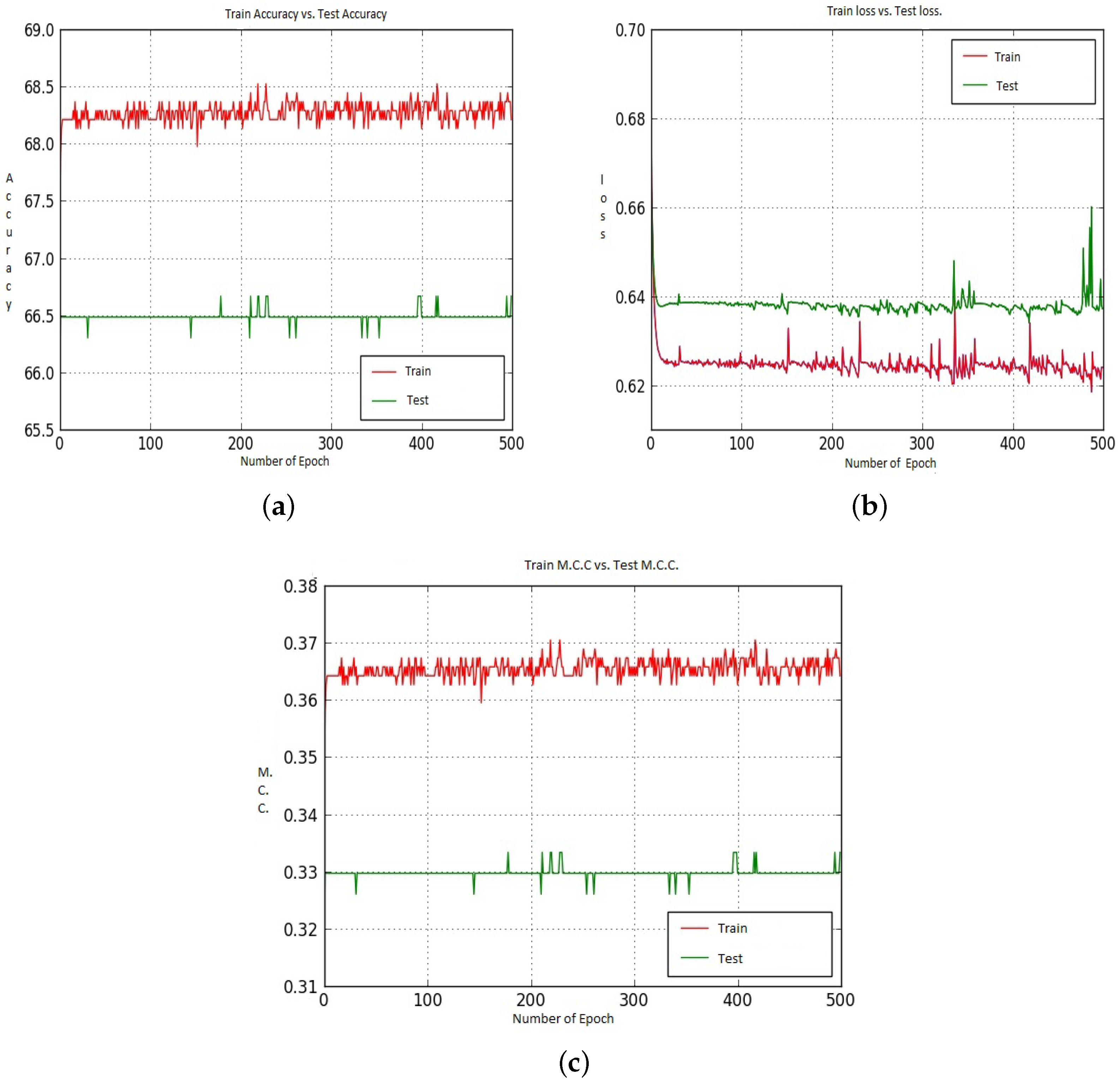
Figure 11 shows the Accuracy, Loss and M.C.C. values for Model-2 on the 40× dataset. Among all the available Models and Cases, CNN-CH provides the worst performance on the 40× dataset when we utilize Model-2. In this particular situation, the Train Accuracy (71.00%) and the Test Accuracy (64.00%) are constant throughout the epochs. For the loss performance, the loss values for Train and Test are also constant throughout the epochs. When we utilised Model-1 and the CNN-CH algorithm on the 40× dataset, we ran our experiment only until about epoch 90 and got quite constant performance.
6.2. Performance of 100× Dataset
For the 100× dataset, when we utilized Model-1 and the CNN-CH algorithm, it provides almost 95.93% Accuracy, along with 94.85% Specificity and 96.36% Recall values (as in Table 4). This indicates that only 5.15% of the Benign data has been misclassified as Malignant data, and 3.64% of Malignant images have been misclassified as Benign images. When we use CNN-I, that is when we utilized raw images as input with Model-1, and the Accuracy is 87.15%. In this particular situation, the Recall value is 93.30%, but the Specificity value is 67.42%, This indicates that almost one third of the Benign images has been misclassified as Malignant images, and this low Specificity value reduces the overall performance. CNN-DC and CNN-DF show similar performance when we utilized Model-1 and the 100×. For Model-2, when we utilized CNN-I, that is when we utilized raw images as input, it produces the best accuracy among all the cases. In this particular case the Specificity value is 81.87% and the Recall value is 88.78%. CNN-DC also provides similar Accuracy to CNN-I; however, it shows very poor specificity performance of 65.71% . For Model-2, CNN-CH provides the worst performance among all the available cases with 67.96% accuracy, 43.00% Specificity and 78.00% Recall values.
Figure 12 and Figure 13 shows the Accuracy, Loss and M.C.C. values for the CNN-CH case on the 100× dataset when Model-1 and Model-2 has been utilized. Initially, up to around epoch 25, the Test Accuracy values show better performance than the Train Accuracy. After that Train Accuracy shows better performance than Test Accuracy. After around epoch 50, Test Accuracy is about 96.00%, and Test Accuracy is about 95.00%. For the loss performance, up to around epoch 21, the Test loss shows better values than the Train loss. However, after epoch 21, the Train loss continuously decreases, whereas the Test loss shows poor performance. For the M.C.C. values, after around epoch 80, the Train M.C.C. value is 0.98 and the Test M.C.C. value is around 0.95.
6.3. Performance of 200× Dataset
For the 200× dataset, when Model-1 and CNN-CH are used together 97.90%, Accuracy is achieved, along with 94.94% Specificity and 98.20% Recall values (as in Table 5). This indicates that almost all the Malignant data have been classified into Malignant, whereas 5.06% of Benign data have been misclassified as Malignant.
When we use Model-2 along with CNN-CH, CNN-CL or CNN-DC, on the 200× dataset, we get very poor performance. In all these three cases, all the data is classified as Malignant data irrespective of reality. In this scenario, the best performance is achieved when we utilized the raw image as input, that means the CNN-I case. In this case, we achieved 86.00% Accuracy, along with 81.87% Specificity and 88.78% Recall values.
Figure 14 shows the Accuracy values for the CNN-CH case on the 200× dataset. Up to around epoch 15, Train Accuracy shows almost the same performance with some exceptions. After that, Train accuracy shows slightly better performance than Test accuracy. Train data shows 100% Accuracy around epoch 90, whereas Test Accuracy shows 97.00%. For the loss performance, as shown in Figure 14b, the Train loss is almost 0, whereas Test loss also shows quite small values but not 0. After around epoch 20, the Train and Test loss values remained constant. After that, the difference between the Train loss value and the Test Loss value is constant. As the epoch proceeds, the Train and Test M.C.C. values increased. Around epoch 85, the Train M.C.C. value touches the highest M.C.C. value, whereas the Test M.C.C. value is around 0.91.
We saw earlier that using CNN-CH, CNN-CL and CNN-DC with Model-2 on the 200× dataset gave very poor performance. Figure 15 shows the Accuracy, Loss and M.C.C. values when we utilized the CNN-CH algorithm on the 200× dataset. For the Accuracy case, Train shows around 69.00% accuracy for all epochs up to 450. On the other hand, Test accuracy remains constant at around 67.5% throughout the epochs. For the loss performance, the difference between the Train and Test losses remains the same throughout all the epochs.
6.4. Performance of 400× Dataset
When we use Model-1 and the CNN-CH algorithm on the 400× dataset, the best performance is achieved (as in Table 6). In this case, the Accuracy is 96.00%, with 90.16% Specificity and 97.79% Recall values. CNN-DF and CNN-DC provide similar performance. When we utilized raw images as an input, the Accuracy achieved is 84.43%. When we use Model-2 and the CNN-CH algorithm on the 400× dataset, the system gives the worst performance, of 67.80% Accuracy with 0.005% Specificity and 100.00% Recall values. Interestingly, CNN-I, CNN-DF, and CNN-DC provide similar performance.
Figure 16 shows the Accuracy, Loss and M.C.C. values for different epochs when we utilized Model-1, CNN-CH and 400× dataset. Figure 16 shows that, up to around epoch 15, the Train and Test Accuracy, Loss and M.C.C. values remain almost the same with some exceptions. After around epoch 15, Train accuracy shows better performance than Test Accuracy. After epoch 50, the Train accuracy becomes constant at around 96.00%, whereas the Test Accuracy shows continually better performance. For the loss, as the epoch proceeds, the difference between the Train loss and the Test loss increased. For M.C.C., the Train M.C.C. value touches around 0.92.
Figure 17 shows Accuracy, Loss and M.C.C. values for different epochs when we utilized Model-2, CNN-CH and the 400× dataset. In this particular scenario, the Train Accuracy keeps around 68.25%, whereas the Test Accuracy is around 66.50%. For the loss case, the Train loss remained around 0.625 and the Test loss remained around 0.63; with some exceptions, those values remain constant for all epochs.
6.5. Required Time and Parameters
Table 7 shows the number of parameters required and the time required to run per epoch for Model-1 and Model-2. Model-1 requires 119,666 parameters for the total operation, whereas Model-2 requires 120,466 parameters.
6.6. Comparison with Findings
Table 8 summarizes a few recent findings of Histopathological breast-image classification. Brook et al. [40] utilize a total of 361 images for their experiment. From each of the images, they have collected 1060 features and as a classifier tool they have utilized the SVM method and obtained 96.40% accuracy. Zhang et al. [41] also perform the classification operation on the same dataset utilizing ensemble methods and have obtained 97.00% Accuracy. Ciresan et al. [42] and Wang et al. [43] both perform their experiments on the ICPR12 dataset where they have utilized global features. The findings of our paper cannot be compared directly with the above-mentioned findings because they have performed their experiment on a different dataset as well as using different classification techniques.
Spanhol et al. [44], Han et al. [45] and Dimitropoulos et al. [46] perform their experiment on the BreakHis dataset. Spanhol et al. [44] obtained the best performance when they utilized the 40× datset and obtained 90.40% accuracy. Han et al. [45] achieve 95.80 ± 3.10% Accuracy on the 40× dataset. Dimitropoulos et al. [46] obtained the best Accuracy performance when they utilized the 100× dataset and the Vector of Locally Aggregated Descriptors (VLAD) method. Our experiment has been performed on the BreakkHis dataset, and obtained the best Accuracy 97.19%, which is almost comparable with the the state-of-the-art findings of Han et al. [45]. Both the work by Spanhol et al. [44], Han et al. [45] and Dimitropoulos et al. [46] finds the Accuracy values only; however, in this paper, we also have findings for the Specificity, Precision, and Recall values along with finding the required number of parameters and the time required to perform the experiment. Besides this, we have also compared our results with Linear Discriminant Analysis (LDA) and Support Vector Machine (SVM) methods and found that our algorithms provide better performance than those two methods.
7. Conclusions
This paper has classified a set of Histopathological breast-images into Benign and Malignant classes. For the classification, the state-of-the-art CNN model has been utilized along with residual blocks. The CNN method generally extracts global features while maintaining the hierarchical structure. However, local features and frequency domain information also carry significant information from images that help significantly for the image classification. Utilizing the benefit of local and frequency domain information as well as hierarchical property of the CNN model, this paper has proposed two different sets of algorithms. The first set of algorithms extracts local feature information, whereas the second set of algorithms extracts frequency-domain information. Feature-extraction based cases suggested two distinct algorithms, where the first algorithm utilized the Contourlet Transform as well as Histogram-based information, whereas the second algorithm is based on the Contourlet Transform and Local Binary Pattern information. Frequency-feature based cases also provide two algorithms, one of the algorithms based on DFT-based information, whereas the second is based on the DCT algorithm. This paper has utilized the BreakHis dataset for the experiment, which contains four datasets. Most of the recent findings on this dataset analyze the Accuracy information. In this paper, along with finding the Accuracy information, we have also found the Precision, Recall, Specificity, M.C.C. and F-1 Score values. Experiment shows that the CNN-CH case provides the best performance on all the available datasets. Specifically, the 200× dataset provides the best performance of the available datasets with 97.19% Accuracy, 94.94% Specificity and 98.20% Recall value. The computational complexity and required time for the classification are two important parameters for the CNN-based image-classification task. In this paper, we have investigated how many parameters are required and the time required for the experiment, which provides information about the complexity of this technique.
Acknowledgments
The work in this paper was supported by an International Macquarie University Research Excellence Scholarship (iMQRES).
Author Contributions
A.-A.N. and Y.K. collected the data. A.-A.N. designed, simulated and conducted the experiment and wrote the paper. Y.K. provided valuable comments on the writing. Both A.-A.N. and Y.N. were responsible for revising the article. The final manuscript has been approved by all the authors.
Conflicts of Interest
The authors declare no conflicts of interest.
References
- Bazzani, A.; Bevilacqua, A.; Bollini, D.; Brancaccio, R.; Campanini, R.; Lanconelli, N.; Riccardi, A.; Romani, D. An SVM classifier to separate false signals from microcalcifications in digital mammograms. Phys. Med. Biol. 2002, 46, 1651–1663. [Google Scholar]
- El-Naqa, I.; Yang, Y.; Wernick, M.; Galatsanos, N.; Nishikawa, R. A support vector machine approach for detection of microcalcifications. IEEE Trans. Med. Imaging 2002, 21, 1552–1563. [Google Scholar] [CrossRef] [PubMed]
- Mhala, N.C.; Bhandari, S.H. Improved approach towards classification of histopathology images using bag-of-features. In Proceedings of the 2016 International Conference on Signal and Information Processing (IConSIP), Vishnupuri, India, 6–8 October 2016. [Google Scholar]
- Dheeba, J.; Selvi, S.T. Classification of malignant and benign microcalcification using svm classifier. In Proceedings of the 2011 International Conference on Emerging Trends in Electrical and Computer Technology, Nagercoil, India, 23–24 March 2011; pp. 686–690. [Google Scholar]
- Taheri, M.; Hamer, G.; Son, S.H.; Shin, S.Y. Enhanced breast cancer classification with automatic thresholding using svm and harris corner detection. In Proceedings of the International Conference on Research in Adaptive and Convergent Systems (RACS‘ 16), Odense, Denmark, 11–14 October 2016; ACM: New York, NY, USA, 2016; pp. 56–60. [Google Scholar]
- Shirazi, F.; Rashedi, E. Detection of cancer tumors in mammography images using support vector machine and mixed gravitational search algorithm. In Proceedings of the 2016 1st Conference on Swarm Intelligence and Evolutionary Computation (CSIEC), Bam, Iran, 9–11 March 2016; pp. 98–101. [Google Scholar]
- Levman, J.; Leung, T.; Causer, P.; Plewes, D.; Martel, A.L. Classification of dynamic contrast-enhanced magnetic resonance breast lesions by support vector machines. IEEE Trans. Med. Imaging 2008, 27, 688–696. [Google Scholar] [CrossRef] [PubMed]
- Angayarkanni, S.P.; Kamal, N.B. Mri mammogram image classification using id3 algorithm. In Proceedings of the IET Conference on Image Processing (IPR 2012), London, UK, 3–4 July 2012; pp. 1–5. [Google Scholar]
- Gatuha, G.; Jiang, T. Evaluating diagnostic performance of machine learning algorithms on breast cancer. In Revised Selected Papers, Part II, Proceedings of the 5th International Conference on Intelligence Science and Big Data Engineering. Big Data and Machine Learning Techniques (IScIDE), Suzhou, China, 14–16 June 2015; Springer-Verlag Inc.: New York, NY, USA, 2015; Volume 9243, pp. 258–266. [Google Scholar]
- Zhang, Y.; Zhang, B.; Lu, W. Breast cancer classification from histological images with multiple features and random subspace classifier ensemble. AIP Conf. Proc. 2011, 1371, 19–28. [Google Scholar]
- Diz, J.; Marreiros, G.; Freitas, A. Using Data Mining Techniques to Support Breast Cancer Diagnosis; Springer International Publishing: New York, NY, USA, 2015; pp. 689–700. [Google Scholar]
- Kendall, E.J.; Flynn, M.T. Automated Breast Image Classification Using Features from Its Discrete Cosine Transform. PLoS ONE 2014, 9, e91015. [Google Scholar] [CrossRef] [PubMed]
- Burling-Claridge, F.; Iqbal, M.; Zhang, M. Evolutionary algorithms for classification of mammographie densities using local binary patterns and statistical features. In Proceedings of the 2016 IEEE Congress on Evolutionary Computation (CEC), Vancouver, BC, Canada, 24–29 July 2016; pp. 3847–3854. [Google Scholar]
- Rajakeerthana, K.T.; Velayutham, C.; Thangavel, K. Mammogram Image Classification Using Rough Neural Network. In Computational Intelligence, Cyber Security and Computational Models; Springer India: New Delhi, India, 2014; pp. 133–138. [Google Scholar]
- Lessa, V.; Marengoni, M. Applying Artificial Neural Network for the Classification of Breast Cancer Using Infrared Thermographic Images. In Computer Vision and Graphics, Proceedings of the International Conference on Computer Vision and Graphics (ICCVG 2016), Warsaw, Poland, 19–21 September 2016; Springer International Publishing: Cham, Switzerland, 2016; pp. 429–438. [Google Scholar]
- Peng, W.; Mayorga, R.; Hussein, E. An automated confirmatory system for analysis of mammograms. Comput. Methods Programs Biomed. 2016, 125, 134–144. [Google Scholar] [CrossRef] [PubMed]
- Silva, S.; Costa, M.; Pereira, W.; Filho, C. Breast tumor classification in ultrasound images using neural networks with improved generalization methods. In Proceedings of the 2015 37th Annual International Conference of the IEEE Engineering in Medicine and Biology Society (EMBC), Milan, Italy, 25–29 August 2015; pp. 6321–6325. [Google Scholar]
- Lopez-Melendez, E.; Lara-Rodriguez, L.D.; Lopez-Olazagasti, E.; Sanchez-Rinza, B.; Tepichin-Rodriguez, E. Bicad: Breast image computer aided diagnosis for standard birads 1 and 2 in calcifications. In Proceedings of the 22nd International Conference on Electrical Communications and Computers (CONIELECOMP 2012), Cholula, Puebla, Mexico, 27–29 February 2012; pp. 190–195. [Google Scholar]
- Fukushima, K. Neocognitron: A self-organizing neural network model for a mechanism of pattern recognition unaffected by shift in position. Biol. Cybern. 1980, 36, 193–202. [Google Scholar] [CrossRef] [PubMed]
- Wu, C.Y.; Lo, S.C.B.; Freedman, M.T.; Hasegawa, A.; Zuurbier, R.A.; Mun, S.K. Classification of microcalcifications in radiographs of pathological specimen for the diagnosis of breast cancer. In Medical Imaging 1994: Image Processing; International Society for Optics and Photonics: Bellingham, WA, USA, 1994. [Google Scholar]
- Arevalo, J.; González, F.A.; Ramos-Pollán, R.; Oliveira, J.L.; Lopez, M.A.G. Representation learning for mammography mass lesion classification with convolutional neural networks. Comput. Methods Programs Biomed. 2016, 127, 248–257. [Google Scholar] [CrossRef] [PubMed]
- Zejmo, M.; Kowal, M.; Korbicz, J.; Monczak, R. Classification of breast cancer cytological specimen using convolutional neural network. J. Phys. Conf. Ser. 2017, 783, 012060. [Google Scholar] [CrossRef]
- Qiu, Y.; Wang, Y.; Yan, S.; Tan, M.; Cheng, S.; Liu, H.; Zheng, B. An initial investigation on developing a new method to predict short-term breast cancer risk based on deep learning technology. In Proceedings of the SPIE Medical Imaging, San Diego, CA, USA, 27 February–3 March 2016. [Google Scholar]
- Jiang, F.; Liu, H.; Yu, S.; Xie, Y. Breast mass lesion classification in mammograms by transfer learning. In Proceedings of the 5th International Conference on Bioinformatics and Computational Biology (ICBCB‘17), Hong Kong, China, 6–8 January 2017; ACM: New York, NY, USA, 2017; pp. 59–62. [Google Scholar]
- Suzuki, S.; Zhang, X.; Homma, N.; Ichiji, K.; Sugita, N.; Kawasumi, Y.; Ishibashi, T.; Yoshizawa, M. Mass detection using deep convolutional neural network for mammographic computer-aided diagnosis. In Proceedings of the 2016 55th Annual Conference of the Society of Instrument and Control Engineers of Japan (SICE), Tsukuba, Japan, 20–23 September 2016; pp. 1382–1386. [Google Scholar]
- Rezaeilouyeh, H.; Mollahosseini, A.; Mahoor, M.H. Microscopic medical image classification framework via deep learning and shearlet transform. J. Med. Imaging 2016, 3, 044501. [Google Scholar] [CrossRef] [PubMed]
- Sharma, K.; Preet, B. Classification of mammogram images by using cnn classifier. In Proceedings of the 2016 International Conference on Advances in Computing, Communications and Informatics (ICACCI), Jaipur, India, 21–24 September 2016; pp. 2743–2749. [Google Scholar]
- Jiao, Z.; Gao, X.; Wang, Y.; Li, J. A deep feature based framework for breast masses classification. Neurocomputing 2016, 197, 221–231. [Google Scholar] [CrossRef]
- Kooi, T.; Litjens, G.; van Ginneken, B.; Gubern-Merida, A.; Sanchez, C.I.; Mann, R.; den Heeten, A.; Karssemeijer, N. Large scale deep learning for computer aided detection of mammographic lesions. Med. Image Anal. 2017, 35, 303–312. [Google Scholar] [CrossRef] [PubMed]
- Anand, S.; Rathna, R.A.V. Detection of architectural distortion in mammogram images using contourlet transform. In Proceedings of the 2013 IEEE International Conference on Emerging Trends in Computing, Communication and Nanotechnology (ICECCN), Tirunelveli, India, 25–26 March 2013; pp. 177–180. [Google Scholar]
- Moayedi, F.; Azimifar, Z.; Boostani, R.; Katebi, S. Contourlet-Based Mammography Mass Classification; Springer: Berlin/Heidelberg, Germany, 2007; pp. 923–934. [Google Scholar]
- Jasmine, J.; Baskaran, S.; Govardhan, A. Nonsubsampled contourlet transform based classification of microcalcification in digital mammograms. Proc. Eng. 2012, 38, 622–631. [Google Scholar] [CrossRef]
- Pak, F.; Kanan, H.R.; Alikhassi, A. Breast cancer detection and classification in digital mammography based on Non-Subsampled Contourlet Transform (NSCT) and Super Resolution. Comput. Methods Programs Biomed. 2015, 122, 89–107. [Google Scholar] [CrossRef] [PubMed]
- Do, M.N.; Vetterli, M. The contourlet transform: An efficient directional multiresolution image representation. IEEE Trans. Image Process. 2005, 14, 2091–2106. [Google Scholar] [CrossRef] [PubMed]
- Burt, P.; Adelson, E. The laplacian pyramid as a compact image code. IEEE Trans. Commun. 1983, 31, 532–540. [Google Scholar] [CrossRef]
- Ojala, T.; Pietikainen, M.; Maenpaa, T. Multiresolution gray-scale and rotation invariant texture classification with local binary patterns. IEEE Trans. Pattern Anal. Mach. Intell. 2002, 24, 971–987. [Google Scholar] [CrossRef]
- Strang, G. The discrete cosine transform. SIAM Rev. 1999, 41, 135–147. [Google Scholar] [CrossRef]
- Marom, N.D.; Rokach, L.; Shmilovici, A. Using the confusion matrix for improving ensemble classifiers. In Proceedings of the 2010 IEEE 26-th Convention of Electrical and Electronics Engineers in Israel, Eliat, Israel, 17–20 November 2010; pp. 555–559. [Google Scholar]
- Spanhol, F.A.; Oliveira, L.S.; Petitjean, C.; Heutte, L. A dataset for breast cancer histopathological image classification. IEEE Trans. Biomed. Eng. 2016, 63, 1455–1462. [Google Scholar] [CrossRef] [PubMed]
- Brook, E.; El-yaniv, R.; Isler, E.; Kimmel, R.; Member, S.; Meir, R.; Peleg, D. Breast cancer diagnosis from biopsy images using generic features and svms. IEEE Trans. Biomed. Eng. 2006. [Google Scholar]
- Zhang, B. Breast cancer diagnosis from biopsy images by serial fusion of random subspace ensembles. In Proceedings of the 2011 4th International Conference on Biomedical Engineering and Informatics (BMEI), Shanghai, China, 15–17 October 2011; pp. 180–186. [Google Scholar]
- Cireşan, D.C.; Giusti, A.; Gambardella, L.M.; Schmidhuber, J. Mitosis Detection in Breast Cancer Histology Images with Deep Neural Networks; Springer: Berlin/Heidelberg, Germany, 2013; pp. 411–418. [Google Scholar]
- Wang, H.; Roa, A.C.; Basavanhally, A.N.; Gilmore, H.; Shih, N.; Feldman, M.; Tomaszewski, J.; Gonzalez, F.; Madabhushi, A. Mitosis detection in breast cancer pathology images by combining handcrafted and convolutional neural network features. J. Med. Imaging 2014, 1, 034003. [Google Scholar] [CrossRef] [PubMed]
- Spanhol, F.A.; Oliveira, L.S.; Petitjean, C.; Heutte, L. Breast cancer histopathological image classification using convolutional neural networks. In Proceedings of the 2016 International Joint Conference on Neural Networks (IJCNN), Vancouver, BC, Canada, 24–29 July 2016; pp. 2560–2567. [Google Scholar]
- Han, Z.; Wei, B.; Zheng, Y.; Yin, Y.; Li, K.; Li, S. Breast cancer multi-classification from histopathological images with structured deep learning model. Sci. Rep. 2017, 7, 4172. [Google Scholar] [CrossRef] [PubMed]
- Dimitropoulos, K.; Barmpoutis, P.; Zioga, C.; Kamas, A.; Patsiaoura, K.; Grammalidis, N. Grading of invasive breast carcinoma through grassmannian vlad encoding. PLoS ONE 2017, 12, e0185110. [Google Scholar] [CrossRef] [PubMed]
- Wang, P.; Hu, X.; Li, Y.; Liu, Q.; Zhu, X. Automatic cell nuclei segmentation and classification of breast cancer histopathology images. Signal Process. 2016, 122, 1–13. [Google Scholar] [CrossRef]
Figure 1.
New cases of breast cancer for women and number of women dying in the last twelve years.

Figure 2.
The left side represents the Benign and right side Malignant histopathological images (This data has been collected from the BreakHis dataset).
Figure 2.
The left side represents the Benign and right side Malignant histopathological images (This data has been collected from the BreakHis dataset).

Figure 3.
Overall image classification model.

Figure 4.
(a) Wedge-shaped frequency response for 4-band decomposition and (b) Contourlet Transform working mechanism.
Figure 4.
(a) Wedge-shaped frequency response for 4-band decomposition and (b) Contourlet Transform working mechanism.

Figure 5.
Feature-Selection Procedure from images when we use DFT and DCT.

Figure 6.
This figure represents the effects of kernel size, the size stride and zero padding in a convolutional operation.
Figure 6.
This figure represents the effects of kernel size, the size stride and zero padding in a convolutional operation.

Figure 7.
Work flow of a Convolutional Neural Network.
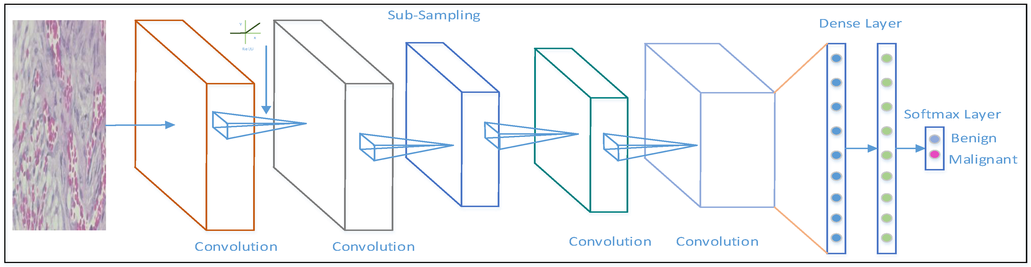
Figure 8.
Architecture of Model-1 on the left and the architecture of Model-2 on the right.
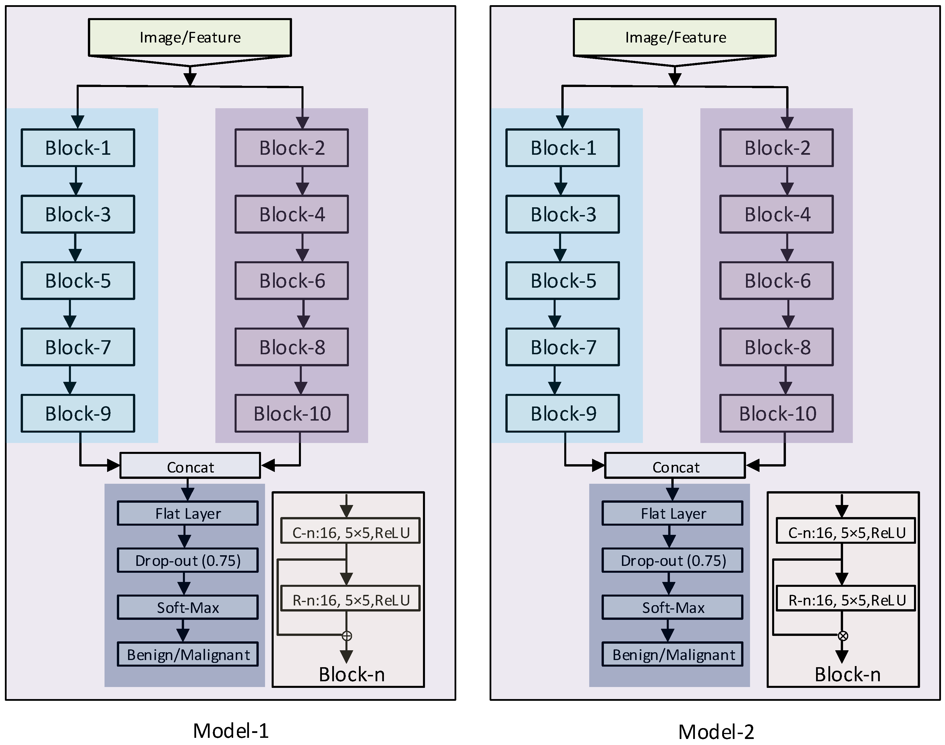
Figure 9.
Confusion matrix.
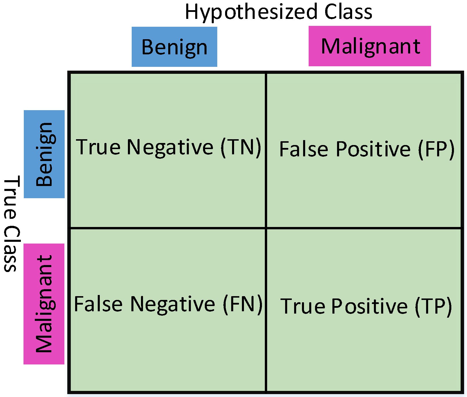
Figure 10.
(a–c) represent the Train and Test Accuracy, Loss and M.C.C. values when we utilized Model-1, CNN-CH on the 40× dataset.
Figure 10.
(a–c) represent the Train and Test Accuracy, Loss and M.C.C. values when we utilized Model-1, CNN-CH on the 40× dataset.
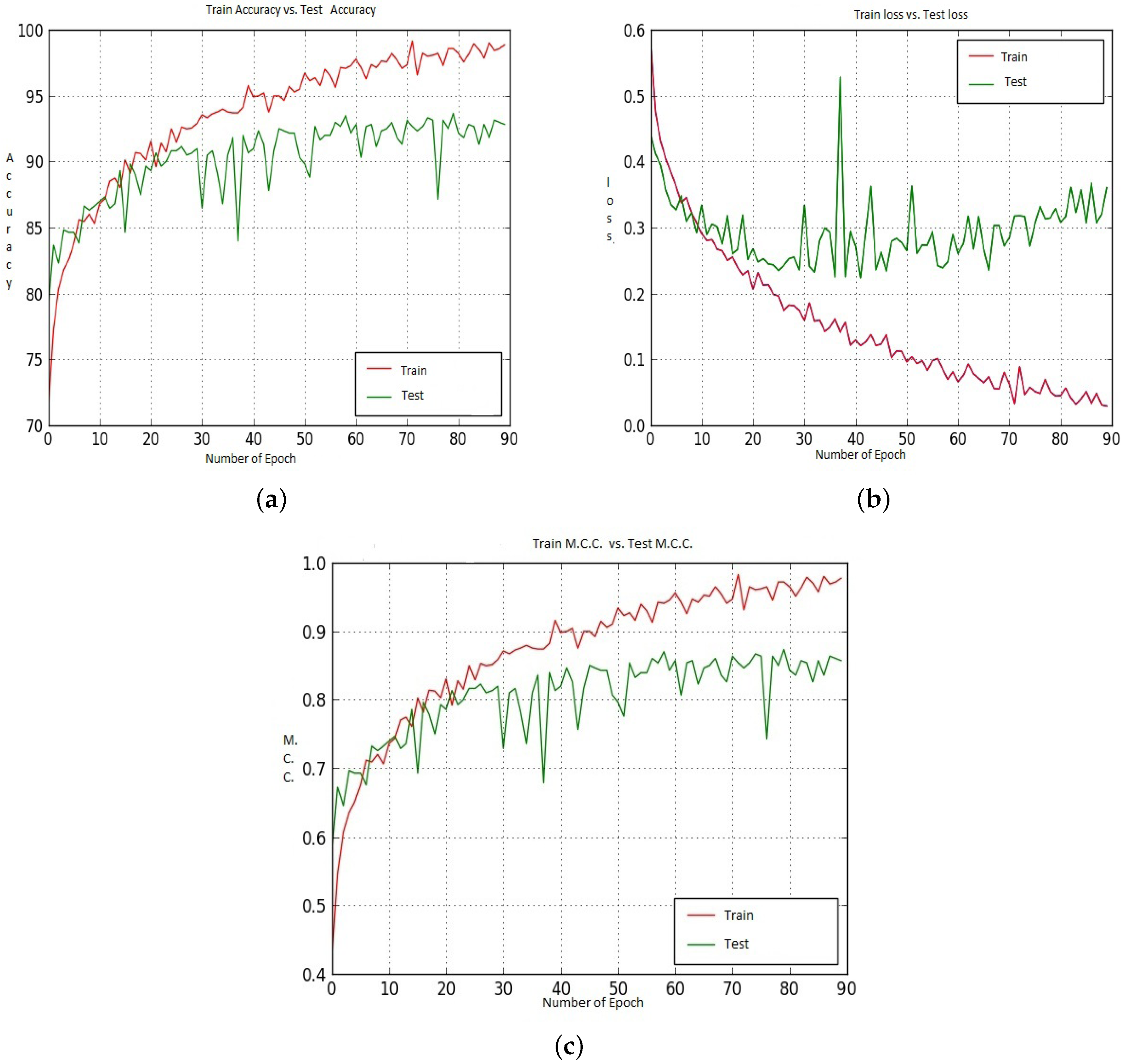
Figure 11.
(a–c) represent the Train and Test Accuracy, Loss and M.C.C. values when we utilized Model-2, CNN-CH on the 40× dataset.
Figure 11.
(a–c) represent the Train and Test Accuracy, Loss and M.C.C. values when we utilized Model-2, CNN-CH on the 40× dataset.
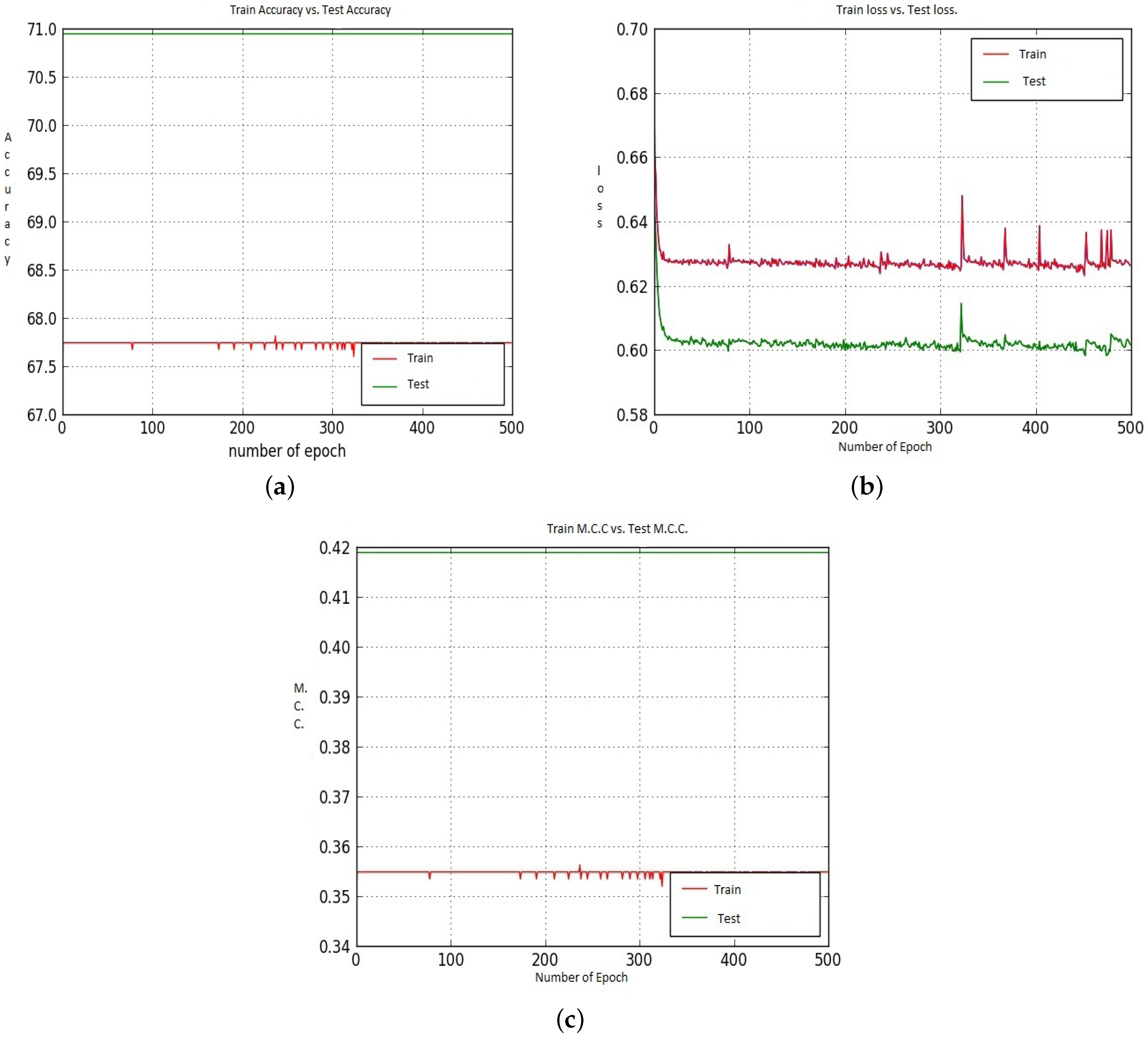
Figure 12.
(a–c) represent the Train and Test Accuracy, Loss and M.C.C. values when we utilized Model-1, CNN-CH on the 100× dataset.
Figure 12.
(a–c) represent the Train and Test Accuracy, Loss and M.C.C. values when we utilized Model-1, CNN-CH on the 100× dataset.
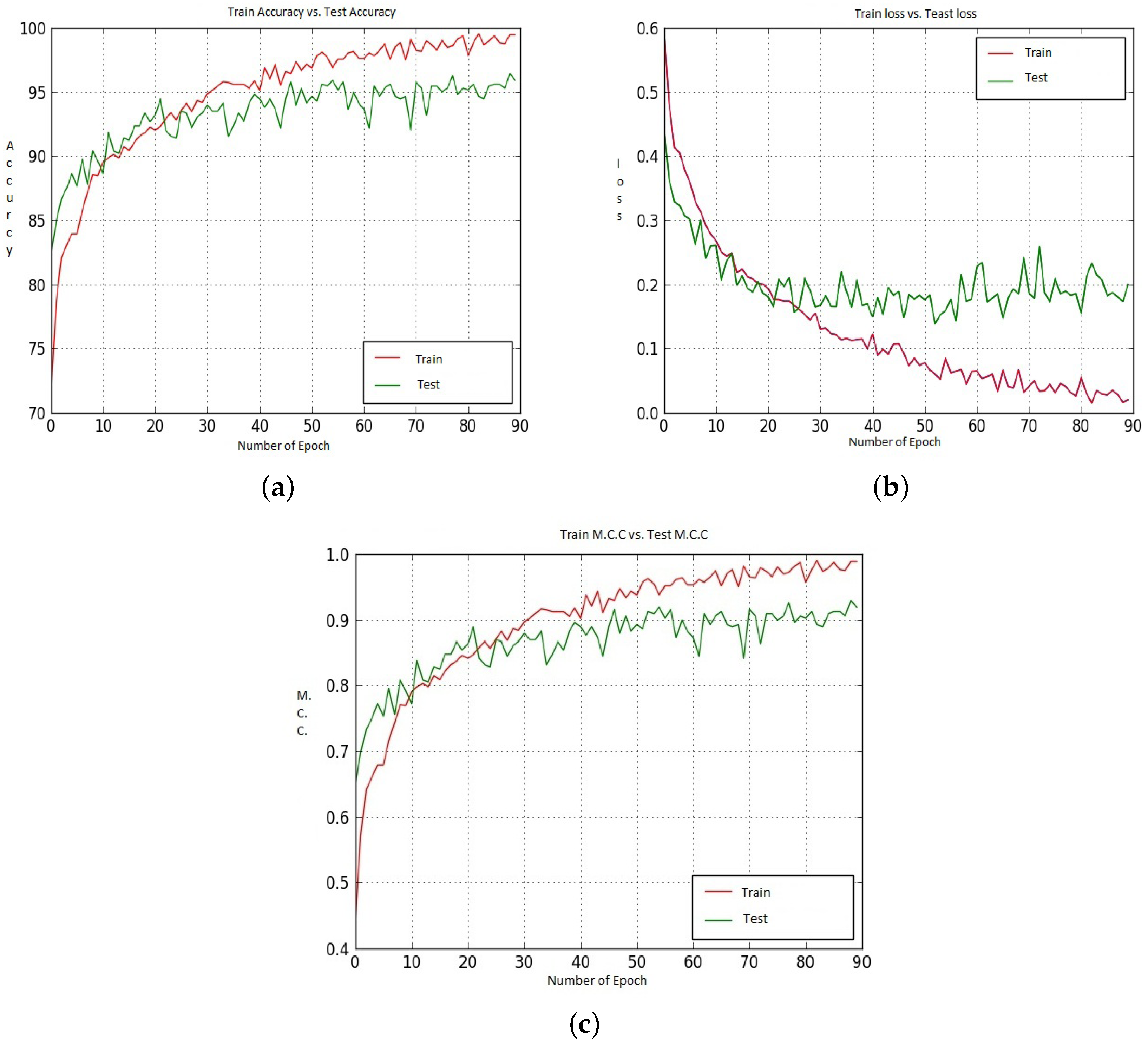
Figure 13.
(a–c) represent the Train and Test Accuracy, Loss and M.C.C. values when we have utilized Model-2, CNN-CH on the 100× dataset.
Figure 13.
(a–c) represent the Train and Test Accuracy, Loss and M.C.C. values when we have utilized Model-2, CNN-CH on the 100× dataset.
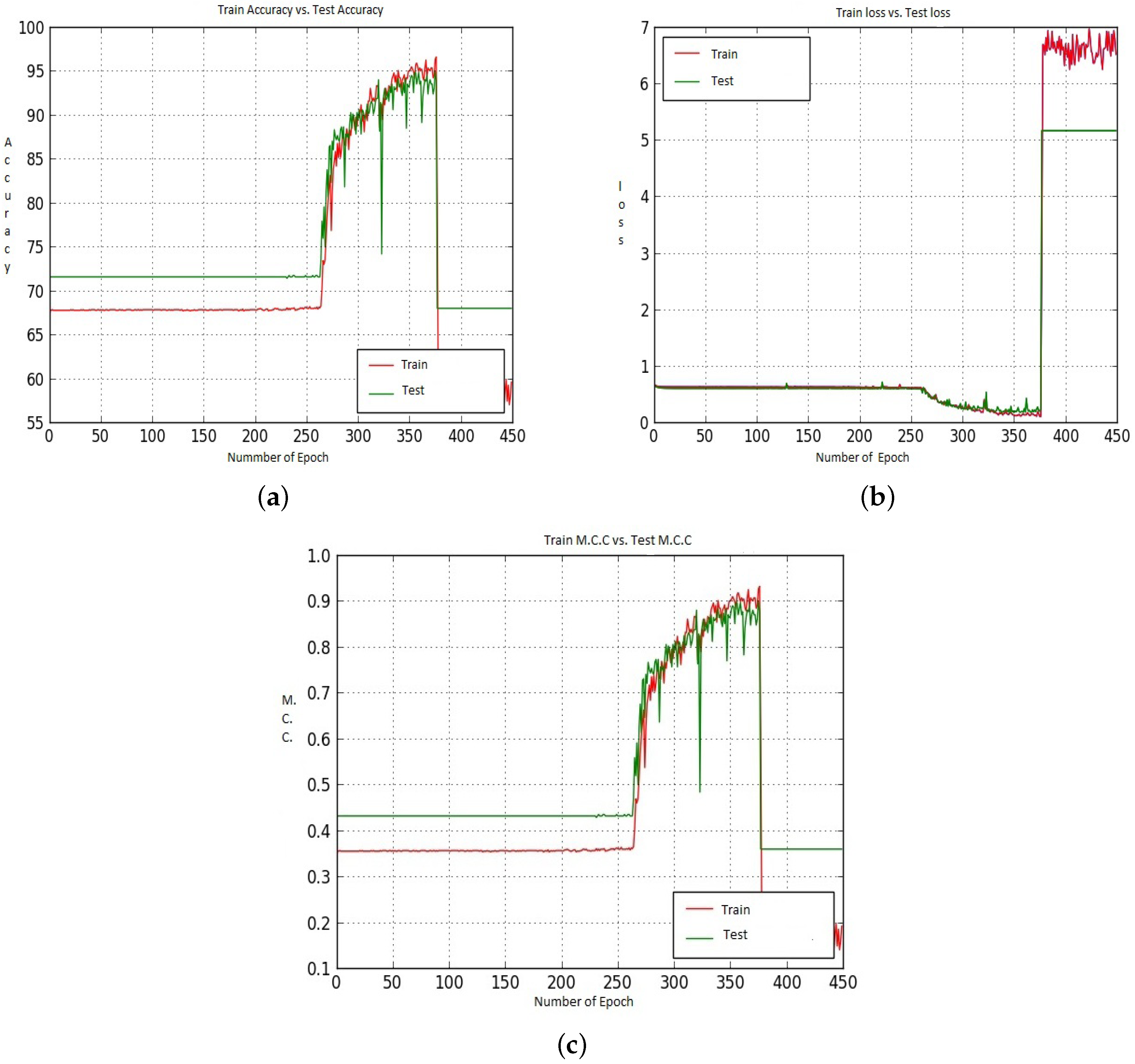
Figure 14.
(a–c) represent the Train and Test Accuracy, Loss and M.C.C. values when we utilized Model-1, CNN-CH on the 200× dataset.
Figure 14.
(a–c) represent the Train and Test Accuracy, Loss and M.C.C. values when we utilized Model-1, CNN-CH on the 200× dataset.
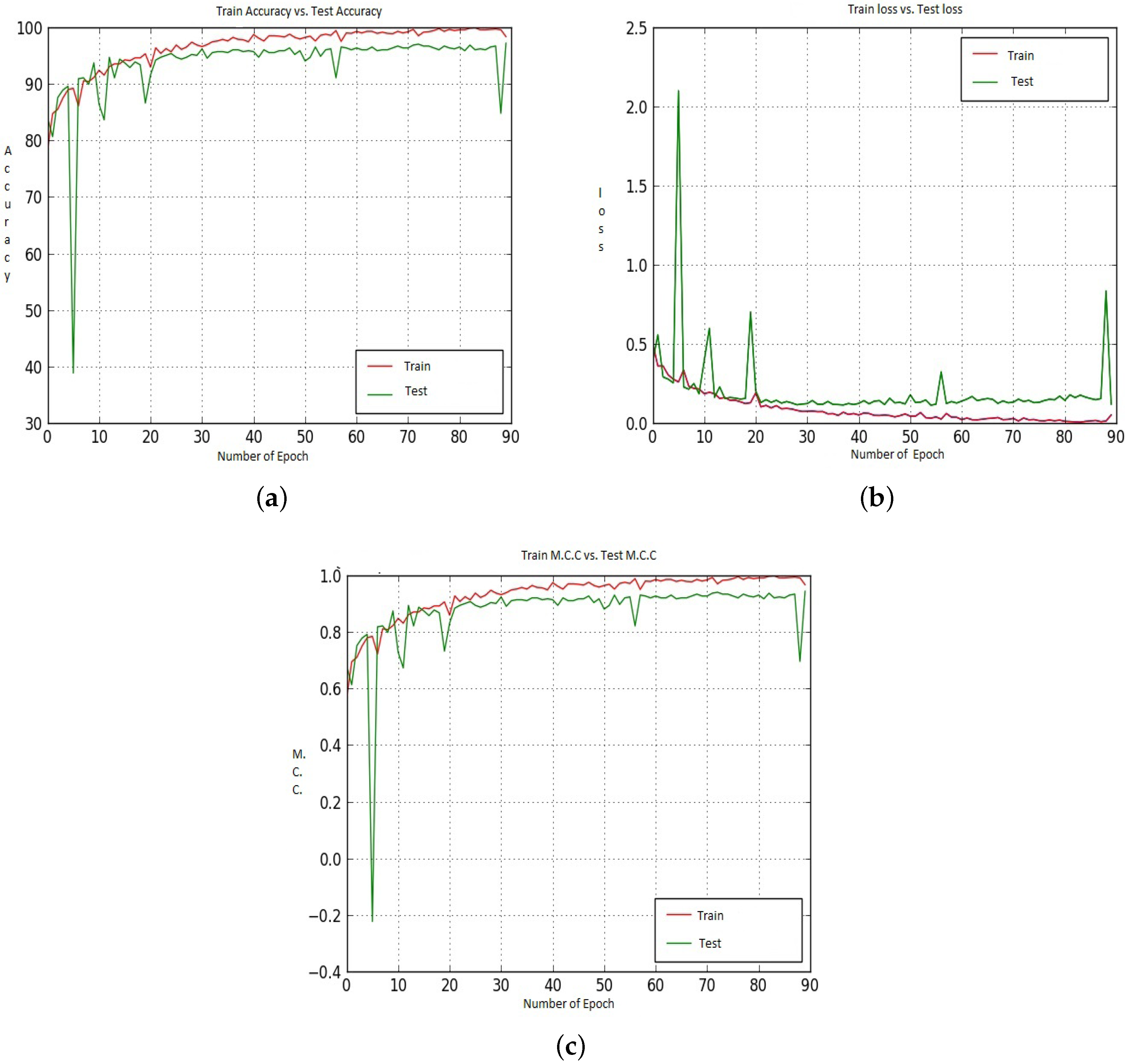
Figure 15.
(a–c) represent the Train and Test Accuracy, Loss and M.C.C. values when we utilized Model-2, CNN-CH on the 200× dataset.
Figure 15.
(a–c) represent the Train and Test Accuracy, Loss and M.C.C. values when we utilized Model-2, CNN-CH on the 200× dataset.
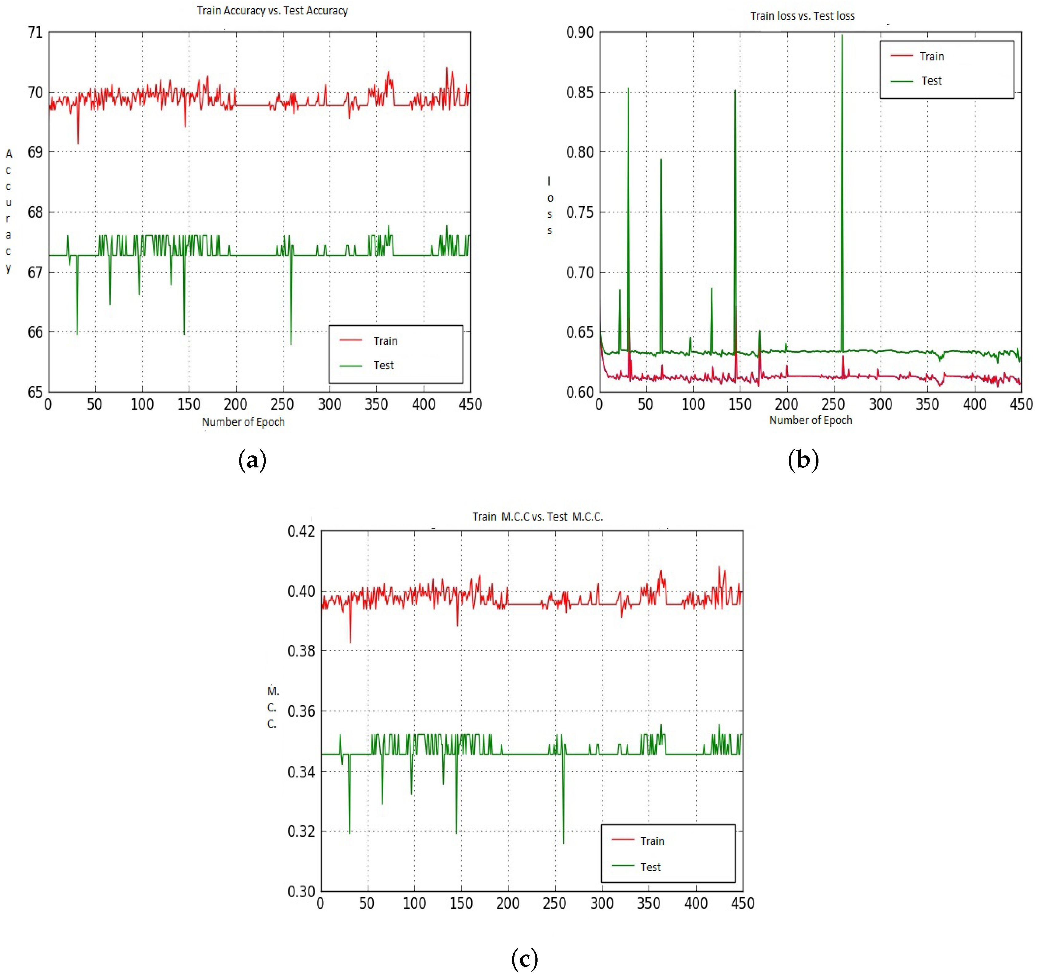
Figure 16.
(a–c) represent the Train and Test Accuracy, Loss and M.C.C. values when we utilized Model-1, CNN-CH on the 400× dataset.
Figure 16.
(a–c) represent the Train and Test Accuracy, Loss and M.C.C. values when we utilized Model-1, CNN-CH on the 400× dataset.

Figure 17.
(a–c) represent the Train and Test Accuracy, Loss and M.C.C. values when we have utilized Model-2, CNN-CH case on the 400× dataset.
Figure 17.
(a–c) represent the Train and Test Accuracy, Loss and M.C.C. values when we have utilized Model-2, CNN-CH case on the 400× dataset.


Table 1.
Number of handcrafted features.
| Case Name | CNN-CH | CNN-CL | CNN-DF | CNN-DC |
|---|---|---|---|---|
| Total Features (Hand Crafted) | 961 | 961 | 2883 | 2883 |
Table 2.
A summary of classification performance measurement parameters.
| Metric Name | Mathematical Expression | Highest Value | Lowest Value |
|---|---|---|---|
| Recall | +1 | 0 | |
| Precision | +1 | 0 | |
| Specificity | +1 | 0 | |
| F-measure | +1 | 0 | |
| M.C.C. | +1 | −1 |
M.C.C. = Matthews Correlation Coefficient.
Table 3.
Performance of various cases on 40× dataset.
| Accuracy % | TNR/Specificity % | FPR (%) | FNR (%) | TPR/Recall (%) | Precision (%) | F-Measure (%) | ||
|---|---|---|---|---|---|---|---|---|
| Model-1 | CNN-CH | 94.40 | 86.00 | 14.00 | 04.00 | 96.00 | 94.00 | 95.00 |
| CNN-CL | 93.32 | 85.05 | 15.95 | 03.20 | 96.70 | 94.00 | 95.00 | |
| CNN-I | 87.47 | 79.31 | 20.68 | 10.00 | 91.00 | 91.00 | 91.00 | |
| CNN-DF | 88.31 | 78.16 | 21.80 | 07.52 | 92.47 | 91.00 | 92.00 | |
| CNN-DC | 86.47 | 74.37 | 25.86 | 08.47 | 91.52 | 90.00 | 91.00 | |
| Model-2 | CNN-CH | 70.00 | 0.00 | 100.00 | 0.00 | 100.00 | 66.00 | 80.00 |
| CNN-CL | 80.30 | 45.77 | 54.07 | 5.6 | 94.35 | 81.00 | 79.00 | |
| CNN-I | 88.31 | 69.45 | 30.45 | 4.00 | 96.00 | 88.50 | 84.78 | |
| CNN-DF | 85.47 | 73.56 | 26.43 | 9.40 | 90.35 | 89.30 | 83.45 | |
| CNN-DC | 86.50 | 52.87 | 47.12 | 3.2 | 96.72 | 83.00 | 90.00 |
(TNR = True Negative Rate, FPR = False Positive Rate, FNR = False Negative Rate, TPR = True Positive Rate).
Table 4.
Performance of various cases on 100× dataset.
| Accuracy % | TNR/Specificity % | FPR (%) | FNR (%) | TPR/Recall (%) | Precision (%) | F-Measure (%) | ||
|---|---|---|---|---|---|---|---|---|
| Model-1 | CNN-CH | 95.93 | 94.85 | 05.15 | 03.64 | 96.36 | 98.00 | 97.00 |
| CNN-CL | 92.00 | 89.10 | 10.90 | 06.70 | 93.30 | 96.00 | 94.00 | |
| CNN-I | 87.15 | 67.42 | 32.50 | 05.00 | 95.00 | 88.00 | 95.00 | |
| CNN-DF | 89.26 | 81.14 | 18.85 | 07.50 | 92.5 | 93.00 | 93.00 | |
| CNN-DC | 87.15 | 78.28 | 21.71 | 09.31 | 90.68 | 91.00 | 91.00 | |
| Model-2 | CNN-CH | 67.96 | 43.00 | 57.00 | 22.00 | 78.00 | 78.00 | 78.00 |
| CNN-CL | 78.53 | 31.42 | 68.52 | 2.73 | 97.27 | 78.00 | 75.00 | |
| CNN-I | 86.12 | 81.87 | 18.18 | 11.26 | 88.78 | 93.00 | 87.00 | |
| CNN-DF | 85.47 | 85.71 | 14.20 | 17.95 | 82.05 | 94.00 | 87.00 | |
| CNN-DC | 86.11 | 65.71 | 34.28 | 6.13 | 93.86 | 87.00 | 90.00 |
Table 5.
Performance of various cases on 200× dataset.
| Accuracy % | TNR/Specificity % | FPR (%) | FNR (%) | TPR/Recall (%) | Precision (%) | F-Measure (%) | ||
|---|---|---|---|---|---|---|---|---|
| Model-1 | CNN-CH | 97.19 | 94.94 | 5.06 | 1.70 | 98.20 | 98.00 | 98.00 |
| CNN-CL | 94.00 | 92.42 | 07.57 | 05.65 | 09.41 | 96.00 | 95.00 | |
| CNN-I | 86.44 | 79.31 | 24.74 | 08.10 | 91.89 | 88.00 | 86.00 | |
| CNN-DF | 87.10 | 88.38 | 11.60 | 13.51 | 86.48 | 94.00 | 90.00 | |
| CNN-DC | 85.61 | 71.71 | 28.28 | 08.00 | 92.00 | 87.00 | 90.00 | |
| CNN-CH | 67.60 | 1.00 | 98.98 | 0.00 | 100.00 | 67.00 | 81.00 | |
| Model-2 | CNN-CL | 67.27 | 0.00 | 100.00 | 0.00 | 100.00 | 67.00 | 80.00 |
| CNN-I | 86.00 | 81.87 | 18.18 | 11.26 | 88.78 | 93.00 | 87.00 | |
| CNN-DF | 85.28 | 72.22 | 27.77 | 8.30 | 96.60 | 87.00 | 89.00 | |
| CNN-DC | 67.00 | 0 | 100.00 | 0 | 100.00 | 67.00 | 80.00 |
Table 6.
Performance of various cases on 400× dataset.
| Accuracy % | TNR/Specificity % | FPR (%) | FNR (%) | TPR/Recall (%) | Precision (%) | F-Measure (%) | ||
|---|---|---|---|---|---|---|---|---|
| Model-1 | CNN-CH | 96.00 | 90.16 | 9.84 | 2.2 | 97.79 | 95.00 | 96.00 |
| CNN-CL | 80.00 | 80.87 | 19.10 | 6.60 | 9.39 | 91.00 | 92.00 | |
| CNN-I | 84.43 | 70.49 | 29.50 | 8.50 | 91.46 | 86.00 | 89.00 | |
| CNN-DF | 93.00 | 87.43 | 12.56 | 7.70 | 92.30 | 94.00 | 93.00 | |
| CNN-DC | 92.00 | 85.70 | 14.20 | 7.10 | 92.20 | 93.00 | 93.00 | |
| Model-2 | CNN-CH | 67.80 | 0.005 | 99.95 | 0.00 | 1.00 | 0.67 | 0.80 |
| CNN-CL | 66.48 | 00.00 | 100.00 | 0.00 | 100/00 | 44.00 | 53.00 | |
| CNN-I | 86.34 | 75.40 | 24.59 | 10.46 | 89.50 | 88.00 | 89.00 | |
| CNN-DF | 87.17 | 74.86 | 25.13 | 6.61 | 93.30 | 88.00 | 91.00 | |
| CNN-DC | 86.26 | 73.22 | 26.77 | 7.11 | 92.83 | 87.00 | 90.00 |
Table 7.
Required time and number of parameters.
| Model | Case | Parameters | Time (s) | Model | Case | Parameters | Time (s) |
|---|---|---|---|---|---|---|---|
| Model-1 | CNN-CH | 120,466 | 45 | Model-2 | CNN-CH | 119,666 | 45 |
| CNN-CL | 119,666 | 45 | CNN-CL | 120,466 | 45 | ||
| CNN-I | 119,666 | 38 | CNN-I | 120,466 | 38 | ||
| CNN-DF | 119,666 | 40 | CNN-DF | 120,466 | 40 | ||
| CNN-DC | 119,666 | 40 | CNN-DC | 120,466 | 40 |
Table 8.
Summary of a few recent findings of Histopathological breast-image classification.
| Authors | Dataset Details | Features | Classification Tool | Number of Classes | Accuracy % | Sensitivity % | Recall % | Precision % | ROC % |
|---|---|---|---|---|---|---|---|---|---|
| Brook et al. [40] | Total Sample: 361 | 1. Local Features 2. 1050 Features. | SVM | 1. 3 Classes a. normal tissue b. carcinoma in situ c. invasive ductal | 96.40 | — | — | — | — |
| Zhang [41] | Total Sample: 361 | 1. Local Feature 2. Texural property 3. Curvelet transform | Ensemble | 1. 3 Classes a. normal tissue b. carcinoma as situ c. invasive ductal | 97.00 | — | — | — | — |
| Ciresan et al. [42] | ICPR12 | 1. Globaal Features | DNN | 2 Classes | — | — | 70.00 | 88.00 | — |
| Wang et al. [43] | ICPR12 | 1. Global Feature 2. Textural Features | — | — | — | — | — | — | 73.45 |
| Wang et al. [47] | Total 68 images | 1. Local Features | SVM | 2 Classes | 95.50 | 99.32 | 94.14 | — | — |
| Spanhol et al. [44] | BreakHis a. 40× b. 100× c. 200× d. 400× | Global Features | CNN | 2 Classes | a. 90.40 b. 87.40 c. 85.00 d. 83.00 | — | — | — | — |
| Han et al. [45] | BreakHis a. 40× b. 100× c. 200× d. 400× | Global Features | VLAD | 2 Classes | a. 95.80 ± 3.1 b. 96.90 ± 1.9 c. 96.70 ± 2.0 d. 94.90 ± 2.8 | — | — | — | — |
| Dimitropoulos et al. [46] | BreakHis a. 40× b. 100× c. 200× d. 400× | Global Features | VLAD | 2 Classes | a. 91.80 b. 92.10 c. 91.40 d. 90.20 | — | — | — | — |
© 2018 by the authors. Licensee MDPI, Basel, Switzerland. This article is an open access article distributed under the terms and conditions of the Creative Commons Attribution (CC BY) license (http://creativecommons.org/licenses/by/4.0/).
Share and Cite
MDPI and ACS Style
Nahid, A.-A.; Kong, Y. Histopathological Breast-Image Classification Using Local and Frequency Domains by Convolutional Neural Network. Information 2018, 9, 19. https://doi.org/10.3390/info9010019
AMA Style
Nahid A-A, Kong Y. Histopathological Breast-Image Classification Using Local and Frequency Domains by Convolutional Neural Network. Information. 2018; 9(1):19. https://doi.org/10.3390/info9010019
Chicago/Turabian StyleNahid, Abdullah-Al, and Yinan Kong. 2018. "Histopathological Breast-Image Classification Using Local and Frequency Domains by Convolutional Neural Network" Information 9, no. 1: 19. https://doi.org/10.3390/info9010019
Note that from the first issue of 2016, this journal uses article numbers instead of page numbers. See further details here.