Forecasting Monthly Electricity Demands by Wavelet Neuro-Fuzzy System Optimized by Heuristic Algorithms

1
Department of Industrial Engineering and Systems Management, Feng Chia University, Taichung 40724, Taiwan
2
Faculty of Information Technology, University of Transport Technology, Hanoi 100000, Vietnam
*
Author to whom correspondence should be addressed.
Information 2018, 9(3), 51; https://doi.org/10.3390/info9030051
Submission received: 12 January 2018
/
Revised: 21 February 2018
/
Accepted: 24 February 2018
/
Published: 28 February 2018
Abstract
:Electricity load forecasting plays a paramount role in capacity planning, scheduling, and the operation of power systems. Reliable and accurate planning and prediction of electricity load are therefore vital. In this study, a novel approach for forecasting monthly electricity demands by wavelet transform and a neuro-fuzzy system is proposed. Firstly, the most appropriate inputs are selected and a dataset is constructed. Then, Haar wavelet transform is utilized to decompose the load data and eliminate noise. In the model, a hierarchical adaptive neuro-fuzzy inference system (HANFIS) is suggested to solve the curse-of-dimensionality problem. Several heuristic algorithms including Gravitational Search Algorithm (GSA), Cuckoo Optimization Algorithm (COA), and Cuckoo Search (CS) are utilized to optimize the clustering parameters which help form the rule base, and adaptive neuro-fuzzy inference system (ANFIS) optimize the parameters in the antecedent and consequent parts of each sub-model. The proposed approach was applied to forecast the electricity load of Hanoi, Vietnam. The constructed models have shown high forecasting performances based on the performance indices calculated. The results demonstrate the validity of the approach. The obtained results were also compared with those of several other well-known methods including autoregressive integrated moving average (ARIMA) and multiple linear regression (MLR). In our study, the wavelet CS-HANFIS model outperformed the others and provided more accurate forecasting.
1. Introduction
Electric energy plays a fundamental role in business operations all over the world. Industries, homes, and services worldwide depend on efficient, reliable, and accessible electricity. Therefore, as electricity has a deep impact on economic activities, the management of electricity and electricity sources must be carefully implemented to guarantee the efficient use of electricity. The key to this is high-quality capacity planning, scheduling, and operations of the electric power systems. Unlike other commodities, electricity cannot be stored. The production, transmission, distribution, and consumption of the electricity are performed simultaneously. As a result, the available capacity generated within the system should meet the system requirements. An accurate knowledge of future electricity demands is necessary for solid capacity planning and scheduling. This leads to a need for reliable electricity demand forecasting to guarantee that electricity generation is sufficient for demand. However, it is difficult to accurately forecast electricity demands because the demand series often contains unpredictable trends, high noise levels, and exogenous variables. Although demand forecasting is difficult to implement, the relevance of forecasting electricity demands has become a much-discussed issue in recent years. This has led to the development of various new tools and methods for forecasting; however, a more accurate forecasting tool is still needed.
Since electricity is a significant driving force behind economic development, the accuracy of demand forecasting plays an important role in leading to the success of efficiency planning. For this reason, electricity analysts need guidelines to select the most appropriate forecasting techniques, to provide accurate forecasts of electricity consumption trends, and to schedule generator planning and maintenance. In general, electricity demand forecasting, accumulated on different time scales, is categorized into short-term, medium-term, and long-term. The short-term is a prediction of the load or electricity that is demanded several hours or days ahead. This prediction is very important for the daily operation of electricity generation and distribution facilities. Short-term demand is generally affected by daily life habits, industrial and economic activities, temperature, and so on. On the other hand, medium-term and long-term demand, which can span periods from a week to several years, is affected by weather conditions, economic and demographic growth, climate change, and so on. Medium-term forecasting provides a prediction of electricity demand for weeks or months. Long-term forecasting predicts the annual power peaks for years in order to plan grid extensions.
Electricity demand forecasting in electric power plants is a complicated task since the demand is affected directly or indirectly by various factors primarily associated with the economy and the weather. In the past, straight line extrapolations of historical electricity consumption trends were adequate methods. However, with the emergence of alternative energies and forms of technology (in electricity supply and end-use), economic fluctuations, industrial development, and global warming issues, effective modeling techniques are increasingly needed. Many researchers have considered forecasting electricity demand by using a variety of modelling techniques. These range from traditional methods, including autoregressive integrated moving average (ARIMA) and multiple linear regression (MLR), which rely on mathematical approaches, to intelligent techniques, such as fuzzy logic and neural networks [1].
In the early development of forecasting approaches, the most commonly used methods were statistical techniques, such as trend analysis and extrapolation. It is relatively easy to apply this kind of method due to its simple calculations. However, as electricity demand is represented by the demands of society, including factories, enterprises, citizens, and the service industry, forecasting power usage requires a certain knowledge of past demand in order to take into account the social evolution of future electricity demand. Therefore, as past data is needed to forecast future data, a time series analysis of electricity demand is usually used to predict future electricity use. Time series forecasting is a powerful tool that is widely used to predict time evolution in many diversified applications. Demand planning, stock prices, sales prediction, or electricity demand forecasting, all provide valuable information to enterprises or traders when making decisions about buying or selling. Different tools, including ARIMA and MLR, have been developed in the field of time series analysis.
Artificial intelligence techniques have been found to be more effective than traditional methods in various application areas [2,3,4], as well as in the electricity demand forecasting area [5,6,7,8,9]. Among these, the neuro-fuzzy system, a hybrid intelligent system, is a combination of artificial neural networks and fuzzy systems and therefore has the advantages of both methods [10,11,12]. Fuzzy systems are appropriate if sufficient expert knowledge about the process is available, while neural networks are useful if sufficient process data is available or measurable. The neuro-fuzzy system can effectively solve non-linear problems [11] and is particularly useful in applications where classical approaches fail or are too complicated to be used. Recently, primitive neuro-fuzzy systems have been widely used in different fields, as well as in electricity demand forecasting [13,14].
From the signal analysis point of view, the electricity demand can be considered as a linear combination of different electricity demand versus time frequencies [15]. Every component of electricity demand corresponds to a range of frequencies. Wavelet transform is especially suitable for transient analysis because of its time-frequency characteristics with automatically adjusted time-window lengths. Recent studies have shown that wavelet transform can be used as an effective tool for capturing important features and characteristics of the electricity demand. On the other hand, several heuristic algorithms, including Gravitational Search Algorithm (GSA), Cuckoo Optimization Algorithm (COA), and Cuckoo Search (CS), all inspired by the behavior of natural phenomena, were developed for solving optimization problems. Through some benchmarking studies, these algorithms have been proven to be powerful and are considered to outperform other algorithms. The GSA, introduced by Rashedi [16], is based on the law of gravity and mass interactions. A comparison of the GSA with other optimization algorithms in solving some problems showed that the GSA had a higher performance [16,17]. The CS, proposed by Yang and Deb [18], was inspired by the particular egg-laying and breeding characteristics of the cuckoo bird. Since then, CS has been used in solving various problems and is considered to outperform other algorithms, such as particle swarm optimization (PSO) and genetic algorithms (GA) [18,19,20,21]. The COA was developed by Rajabioun [22]. The comparisons of the COA with standard versions of PSO and GA also showed that the COA has superiority in fast convergence and global optimal achievement [22,23].
The merit of recently developed heuristic algorithms, wavelet transform, and the success of neuro-fuzzy systems have encouraged us to combine these techniques for forecasting electricity demand. First, in the proposed studies, the historical demand will be decomposed to an approximate part of a particular signal that is associated with low frequencies, and several detailed parts associated with high frequencies by a wavelet transform. Second, the neuro-fuzzy system optimized by heuristic algorithms will be used to forecast the approximate part of the future demand. Finally, the electricity demand will be forecasted by summing the predicted approximate part and the weighted detail parts. To the best of our knowledge, this is the first study that suggests that combination for forecasting model. The contribution of this study is not only the application of the proposed method for forecasting electricity demand, but also for other forecasting problems. In this study, several models for electricity demand forecasting will be developed and tested to provide predictions. Then, the forecasting (output) values of the models will be compared with the actual value. The determination of an appropriate forecasting model will be based on the error criteria, such as root mean squared error (RMSE) and mean absolute percentage error (MAPE). In order to show the validity and the practicality of the proposed method, we will apply the proposed approach to the real dataset. Furthermore, the performance of the proposed approach will be compared to that of other techniques.
The research is organized into six sections. After the introduction in Section 1, the literature review is provided in Section 2. Section 3 is dedicated to the brief introduction of a neuro-fuzzy system, wavelet transform and three heuristic algorithms including GSA, COA, and CS. Section 4 is devoted to presenting the research design. Experimental results and discussion are in Section 5. Finally, Section 6 presents the conclusion.
2. Literature Review
A variety of methods and techniques have been applied to electricity demand forecasting with varying degrees of success. This section aims at reviewing previous studies in this field. Zahedi [14] proposed a model for estimating electricity demand in Ontario, Canada from 1976 to 2005. In their model, they designed an ANFIS network (adaptive neuro fuzzy inference system) that mapped six parameters as input variables (i.e., employment, gross domestic product—GDP, dwelling, population, heating degree day—HDD, and cooling degree day—CDD) to electricity demand as the output variable. The network had good forecasting capacity with an mean squared error (MSE) of 0.0016. Also, through a comparative analysis, the ANFIS outperformed other methods, including regression and artificial neural network (ANN) models. Iranmanesh [13] proposed a long-term energy demand forecasting approach based on a local linear neuro-fuzzy model. The model was utilized to forecast monthly crude oil, gasoline and natural gas demand of the United States in 2008, 2009 and 2010, respectively. The historical demand data and other exogenous variables were used as inputs. The forecasting results indicated that the proposed approach can be effectively used in real world energy demand forecasting applications. Kazemi [24] presented a genetic-based adaptive neuro-fuzzy inference system (GBANFIS) to construct short-term load forecasting expert systems and controllers. In this model, the adaptive neuro-fuzzy inference system was used to evolve the initial knowledge-base of the expert system. The model was applied to solve the Iranian monthly electrical load forecasting problem. The obtained results were compared with those of time-series, regression, GA, simulated-based GA, ANN, simulated-based ANN, fuzzy decision tree, and simulated-based adaptive neuro-fuzzy inference system approaches. The comparative analysis showed that their proposed method outperforms other models. Chaturvedi [25] conducted short term load forecasting by the use of wavelet transform and neuro-fuzzy systems. Wavelet transform was used to extract the featured coefficients from data, and the neuro-fuzzy system was utilized to predict the trends in electricity demand. Chaturvedi [25] used data collected from the Gujarat system. The experiment showed that the combination of wavelet transform and the neuro-fuzzy system provided better results than the neuro-fuzzy system. Akdemir and Çetinkaya [26] used ANFIS to solve long term forecasting problems for energy demand from 2003 to 2025. The results were compared to those obtained by other mathematical methods to show their validity. Based on the results, it can be concluded that it is possible to use forecasting methods for long term electricity demand forecasting. Zhao et al. [27] made a combination of the logistic curve model and the multi-dimensional forecasting model to improve forecasting performance. In order to verify the effectiveness, the combined model was applied to Hubei Province, showing a higher forecasting accuracy. Chen et al. [28] used artificial neural networks (ANN) trained by different recent heuristic algorithms to estimate monthly electricity demands. The proposed models are applied to Hanoi, Vietnam. The study demonstrated that the ANN trained by Cuckoo Optimization Algorithm outperformed the others and provides more accurate forecasting than traditional methods. Liang and Liang [29] proposed a new mathematical hybrid method based on the modified grey model GM(1,1) model, the Logistic model, and the induced ordered weighted harmonic averaging operator to forecast electricity demand. The results demonstrated that the hybrid model is superior to both single-forecasting approaches and traditional joint-forecasting methods, thus providing the high forecasting accuracy. A dynamic artificial neural network system was proposed for medium term load modeling and forecasting [30]. All models were validated with actual data from the Taiwan Power Company. The model offered an alternative method to the ANN-based method, and is shown to be more effective in load forecasting. The Gaussian Process regression (GPR) for performing monthly load forecasting for a year ahead was introduced and tested on the real dataset [31]. Results showed the superiority of the GPR forecasting over that of the linear regression, however, a dependence of GPR on selection of kernel is observed. Alamaniotis et al. [32] applied two types of kernel machines, including Gaussian process regression (GPR) and relevance vector regression (RVR), for medium term load forecasting (MTLF) and their performance was recorded based on a set of historical electricity load demand data. Results demonstrated the superiority of RVR over the other forecasting models in performing MTLF.
Regarding wavelet transform, there is very little research related to electricity demand forecasting. Moreno-Chaparro [33] showed that wavelet transform can be efficiently utilized to determine demand trends and high frequency components. In addition, the electricity demand can be assumed to be a linear combination of some components. Therefore, in our research, a combination of a neuro-fuzzy system and wavelet transform will be used to analyze, decompose, and develop a new method for forecasting the future electricity demand. Gao and Tsoukalas [34] presented the neural-wavelet approach and its implementation to load identification and forecasting. The developed model was shown capable of handling the nonlinearities involved and provided a tool for intelligent demand-side management.
The above-mentioned studies reveal that neuro-systems have been successfully used in the area of electricity demand forecasting. In order to increase the reliability of forecasting results of the neuro-fuzzy systems, attention is needed to focus on optimizing the parameters of the model and improving the quality of the information available for the forecasting model. The best way to make an accurate forecast is by utilizing a combination of different techniques [33]. However, the published literature only provides forecasting models based on the neuro-fuzzy system or the wavelet neuro-fuzzy system without the combination of heuristic algorithms. Considering recent literature, there is still room for improving the neuro-fuzzy systems for the problem of electricity demand forecasting. In this research we will propose an approach to improve the neuro-fuzzy system by the incorporation of the recent heuristic algorithm and wavelet transform for forecasting electricity demand. This approach will make use of the ability of all these techniques and this development has not been previously reported. We believe this proposed novel approach not only can be used for short-term, mid-term, and long-term electricity demand forecasting, regionally or nationally, but also has the potential to be applied in other applications.
3. Preliminaries
3.1. Neuro-Fuzzy System
3.1.1. Fuzzy Inference System
The fuzzy inference system (FIS) is a process of mapping from a given input to an output using the theory of fuzzy sets. Figure 1 shows an example of the fuzzy inference system. In general, the main steps performed in the FIS are as follows:
- The fuzzification interface transforms each crisp input variable into a membership grade based on the membership functions defined.
- The inference engine then conducts the fuzzy reasoning process by applying the appropriate fuzzy operators in order to obtain the fuzzy set to be accumulated in the output variable.
- The defuzzification interface transforms the fuzzy output into a crisp output by applying a specific defuzzification method
The two types of fuzzy inferences most commonly used are the Mamdani method and the Sugeno method [35]. The difference between these two methods is the specification of the consequent part. In the Mamdani method [36], consequents are fuzzy sets, and the final crisp output of the Mamdani method is based on defuzzification of the overall fuzzy output using various types of defuzzification methods. Whereas, in the Sugeno method [37], consequents are real numbers, which can be either linear or constant. The final output (known as a singleton output membership function) is the weighted average of each rule’s output.
The key success of and interest in FIS are that it offers the capability to deliver the process of turning data into knowledge that can be understood by people. The representation of rules to express the behavior of the system is constructed from human expert knowledge [38]. FISs have been widely used to solve different classification problems. However, the reliance on experts to form the fuzzy rules (to define the membership functions, fuzzy operators, and the knowledge base) and lack of learning capabilities, are some of the limitations of FISs [39].
There are three types of Fuzzy inference systems. They are:
- Mamdani fuzzy model
- Takagi-Sugeno fuzzy model
- Tsukamoto Model fuzzy model
The Mamdani fuzzy inference system was first proposed by Mamdani [40] as an attempt to control a steam engine and boiler combination from a set of linguistic control rules obtained from experienced human operators. In this model both input and output membership functions are in the form of linguistic variables. To implement this type of fuzzy model one must go through the following six steps.
- Step 1:
- Setting the fuzzy rules: Fuzzy rules are the conditional statements that define the relationship between the input membership functions and output membership functions. For example, if input 1 is low and input 2 is high then output is high. Here the values of low, medium and high to the inputs are called linguistic variables or the membership functions. Expert Knowledge is used for this purpose
- Step 2:
- Fuzzification: It is the process of converting crisp data into fuzzy data. The input data is classified into input membership functions which can be linguistic variables such as low, medium, etc. This is usually done on the basis of expert human knowledge.
- Step 3:
- Combining the fuzzified inputs according to the fuzzy rules to establish rule strength.
- Step 4:
- Finding the consequence of the rules by combining the rule strength and the output membership function.
- Step 5:
- The outputs of all the fuzzy rules are calculated and combined to get an output distribution.
- Step 6:
- Defuzzification: Usually a crisp output is required in most of the applications. Defuzzification is the process of converting fuzzy data (Output distribution) to crisp data (single value). There are many methods which can be used for this purpose. Some of the commonly used methods are Center of Mass, Mean of the Maximum etc.
Sugeno fuzzy model also known as TSK (Takagi Sugeno Kang) fuzzy model was proposed by Takagi, Sugeno and Kang in an effort to develop a systematic approach to generate fuzzy rules from a given input and output data set. In this model the input membership functions can be linguistic variables, but the output must be linear or constant. In this model the fuzzy rules are of the form.
If x is A and y is B then z = f(x,y), where A and B are the fuzzy input membership functions and z = f(x,y) is the crisp output. Usually the output is a polynomial expression of x and y. The order of the polynomial defines the order of the model. Since the output of each rule is a crisp value, the overall output is calculated as the weighted average of all the rules. Furthermore, because the output is a crisp value there is no need of defuzzification in this model, and thus reducing the complexity when compared to Mamdani model.
If z = k (constant), then it is known as zero order Sugeno model.
If z = px + qy + r, then it is a first order polynomial of inputs and it is called as first order Sugeno model.
Tsukamoto Fuzzy Model is proposed by Tsukamoto [41]. The consequent of each fuzzy if-then rule is represented by a fuzzy set with a monotonical membership function. As a result, the inferred output of each rule is defined as a crisp value induced by the rule’s firing strength. The overall output is taken as the weighted average of each rule’s output. Since each rule infers a crisp output, the Tsukomoto fuzzy model aggregates each rule’s output by the method of weighted average and thus avoids the time-consuming process of defuzzification. The Tsukamoto fuzzy model is not often used since it is not as transparent as either the Mamdani or Sugeno fuzzy model [42].
3.1.2. Adaptive Neuro-Fuzzy Inference System (ANFIS)
Neural networks and fuzzy set theory, which are both computational intelligence techniques, are tools for establishing intelligent systems. A FIS employs fuzzy if-then rules when acquiring knowledge from human experts to deal with imprecise and vague problems. As mentioned, fuzzy systems cannot learn from or adjust themselves. On the other hand, a neural network has the capacity to learn from its environment, self-organize, and adapt in an interactive way. For these reasons, a neuro-fuzzy system, which is the combination of a fuzzy inference system and a neuron network, has been introduced to produce a complete fuzzy rule-based system [43,44]. The advantages of neural networks and fuzzy systems can be integrated into a neuro-fuzzy approach. Fundamentally, a neuro-fuzzy system is a fuzzy network that has its function as a fuzzy inference system. The system can overcome some limitations of neural networks, as well as the limits of fuzzy systems [45,46], when it has the capacity to represent knowledge in an interpretable manner and the ability to learn. Most neuro-fuzzy system research follows a structure similar to that proposed by Takagi and Hayashi [47]. There are several ways to combine neural networks and fuzzy systems. In general, the neuro-fuzzy system can be classified into three types, dependent on how the combinations between the neural network system and fuzzy system are performed. These three types are as follows [48]:
- Cooperative Neuro-Fuzzy System: The neural network is used at the initial phase to determine the fuzzy set and/or fuzzy rules, and then the fuzzy system is fully utilized for execution.
- Concurrent Neuro-Fuzzy System: Neural networks are used to provide input for a fuzzy system, or to change the output of the fuzzy system. In this case, the parameters of the fuzzy system are not changed by the learning process.
- Hybrid Neuro-Fuzzy System: A fuzzy system uses a learning algorithm inspired by the neural networks to determine its parameters through pattern processing.
In this study, the third type, the hybrid neuro-fuzzy system will be applied to develop prediction models. Among the third type of neuro-fuzzy systems, the ANFIS, introduced by Jang [43], has been one of the most common tools. In the FIS, the fuzzy if-then rules are determined by experts, whereas in the ANFIS, the model itself automatically produces adequate rules with respect to input and output data and facilitates the learning capabilities of neural networks.
ANFIS is a multilayer feed-forward neural network, which employs neural network learning algorithms and fuzzy reasoning to map from input space to output space. The architecture of ANFIS includes five layers, namely the fuzzification layer, the rule layer, the normalization layer, the defuzzification layer, and a single summation node. To present the ANFIS architecture and simplify the explanations, we assume that the FIS has two inputs (x1 and x2), two rules, and one output (y) as shown in Figure 2. Each node within the same layer performs the same function. The circles are used to indicate fixed nodes, while the squares are used to denote adaptive nodes. A FIS that has two inputs and two fuzzy if-then rules [49] can be expressed as:
where x1 and x2 are the inputs; A1, A2, B1, B2 are the linguistic labels; pi, qi, and ri, (i = 1 or 2) are the consequent parameters [43] that are identified in the training process; and y1 and y2 are the outputs within the fuzzy region. Equation (1) represents the first type of fuzzy if-then rules, in which the output part is linear. The output part can also be a constant [37], and is represented as
where Ci (i = 1 or 2) are constant values. Equation (2) represents the second type of fuzzy if-then rules. For complicated problems, the first type of if-then rules is widely utilized to model the relationships of inputs and outputs [50]. In this research, a linear function will be used for the output.
Rule 1: If x1 is A1 and x2 is B1 then y1 = p1x1 + q1x2 + r1,
Rule 2: If x1 is A2 and x2 is B2 then y2 = p2x1 + q2x2 + r2,
Rule 2: If x1 is A2 and x2 is B2 then y2 = p2x1 + q2x2 + r2,
Rule 1: If x1 is A1 and x2 is B1 then y1 = C1,
Rule 2: If x1 is A2 and x2 is B2 then y2 = C2,
Rule 2: If x1 is A2 and x2 is B2 then y2 = C2,
A brief description of each layer’s function is as follows:
Layer 1—fuzzification layer: Every node in this layer is a square node. The nodes produce the membership values. Outputs obtained from these nodes are calculated as follows:
where O1,i denotes the output of node i in layer 1, and µAi(x1) and µBi−2(x2) are the fuzzy membership functions of Ai and Bi−2. The fuzzy membership functions can be in any form, such as triangular, trapezoidal, or Gaussian functions.
O1,i= µAi(x1) for i = 1, 2 or
O1,i= µBi−2(x2) for i = 3, 4,
O1,i= µBi−2(x2) for i = 3, 4,
Layer 2—rule layer: Every node in this layer is a circular node. The output is the product of all incoming inputs.
where O2,i denotes the output of node i in layer 2, and wi represents the firing strength of a rule.
O2,i= wi = µAi(x1) × µBi(x2) for i = 1, 2,
Layer 3—normalization: Every node in this layer is a circular node. Outputs of this layer are called normalized firing strengths. The i-th node is calculated by the i-th node firing strength to the sum of all rules’ firing strengths.
where O3,i denotes the output of node i in layer 3, and is the normalized firing strength.
Layer 4—defuzzification layer: Every node in this layer is an adaptive node with a node function.
where O4,i denotes the output of node i in layer 4, is the output of layer 3, and {pi, qi, ri} (in Equation (6)) is the parameter set. Parameters in this layer are consequent parameters of the Sugeno fuzzy model.
Layer 5—a single summation node: The node is a fixed node. This node computes the overall output by incorporating all the incoming signals from the previous layer:
where O5,i denotes the output of node i in layer 5. The results are then defuzzified using a weighted average procedure.
The ANFIS architecture has two adaptive layers: layer 1 and layer 4. Layer 1 has parameters related to the fuzzy membership functions and layer 4 has parameters {pi, qi, ri} related to the polynomial. The aim of the hybrid learning algorithm in the ANFIS architecture is to adjust all of these parameters in order to make the output match the training data. Adjusting the parameters includes two steps. In the forward pass of the learning algorithm, the premise parameters are fixed, functional signals go forward till layer 4, and the consequent parameters are identified by the least squares method to minimize the measured error. In the backward pass, the consequent parameters are fixed, the error signals go backward, and the premise parameters are updated by the gradient descent method [42]. This hybrid learning algorithm is able to decrease the complexity of the algorithm and increase learning efficiency [51]. The hybrid learning algorithm will be utilized in this study due to this advantage.
There are different types of membership functions that can be used in layer 1. Some of the commonly used membership functions are triangular membership function, trapezoidal membership function, bell shaped membership function, and Gaussian membership function.
According to Güneri [52], an excessive number of inputs in the ANFIS structure makes the system complicated and limits its applicability (also known as the curse-of-dimensionality problem). In addition, many studies have pointed out that ANFIS gives better solutions with a simple structure. To deal with this issue, several low-dimensional rule bases should be arranged in a hierarchical structure [53]. For modeling a hierarchical ANFIS (HANFIS), it is necessary to identify a suitable hierarchical structure, the number of inputs for each sub-ANFIS model, and a rule base for each sub-ANFIS model. Suppose that there are five inputs. The two-layer HANFIS model will be employed is shown as in Figure 3.
3.1.3. Rule Selection for Adaptive Neuro-Fuzzy Inference System (ANFIS)
In a conventional FIS, the number of rules is commonly decided by experts who are familiar with the target system to be modeled. In ANFIS simulation, however, no expert is available, and the number of membership functions (MFs) assigned to each input variable is chosen empirically by plotting the data sets and examining them visually, or simply by trial and error. For datasets with more than two inputs, visualization techniques are not very effective, and therefore we often have to rely on trial and error. This situation is similar to that of neural networks; there is just no simple way to determine the minimal number of hidden units needed in advance to achieve a desired performance level.
When identifying the rule base for ANFIS, we are under the circumstance of: (1) there are no standard methods for transforming human knowledge or experience into the rule base; and (2) it is necessary to tune the membership functions to maximize the performance and minimize the errors [43]. There are several techniques for determining the numbers of MFs and rules. The most common methods are grid partitioning and scatter partitioning.
The grid partition method divides the data space into rectangular sub-spaces using an axis-paralleled partition based on a pre-defined number of membership functions and the type of each dimension. Premise fuzzy sets and parameters are calculated using the least square estimate method based on the partition and membership function. When constructing the fuzzy rules, consequent parameters in the linear output membership function are set at zero. Therefore, it is necessary to identify and refine the parameters by the use of ANFIS. The combination of grid partition and ANFIS can be found in the literature [54]. The application of grid partition in FIS is limited by the curse-of-dimensionality, since the number of fuzzy rules increases exponentially when the number of input variables increases. If there are m membership functions for every input variable and a total of n input variables, the number of fuzzy rules is mn. Hence, this method is only suitable for simple problems with a small number of input variables.
In order to eliminate the problems associated with grid-partitioning, other ways of dividing the input space into rule patches have been proposed. This approach allows the IF-parts of the fuzzy rules to be positioned at arbitrary locations in input space. If the rules are represented by n-dimensional Gaussians or normalized Gaussians, the centers of the Gaussians are not anymore confined to corners of a rectangular grid. Rather, they can be chosen freely.
The scatter partitioning method includes the fuzzy-C means (FCM) clustering method and the subtractive clustering method. FCM, also known as fuzzy ISODATA (Iterative Self-Organizing Data Analysis Technique Algorithm) [55], partitions a collection of n vectors into C fuzzy groups and finds a cluster center in each group so that a cost function of dissimilarity measure is minimized. FCM also employs fuzzy partitioning so that a given data point can belong to several groups, with a degree of belongingness specified by membership grades between 0 and 1. Here, the number of cluster centers represents the number of rules and the researchers can determine the number of rules.
When there is no clear idea about how many clusters there should be for a given set of data, subtractive clustering is a fast, one-pass algorithm for estimating the number of clusters and the cluster centers for a set of data [50,56]. Subtractive clustering method was proposed by Chiu [57] by extending the mountain clustering method [58]. It clusters data points by measuring their potential in the feature space. Subtractive clustering method assumes that each data point is a potential cluster center and calculates the potential for each data point based on the density of surrounding data points. The data point with the highest potential is chosen as the first cluster center, and the potential of data points near the first cluster center (within the neighboring radius) are removed.
In a set of n data points, (x1, x2, ..., xn), the potential of xi to be a cluster center is calculated as follows:
where Di is the potential value of the i-th data point and ra denotes the neighboring radius. If a point has more points within its neighboring radius, it will have a higher potential value.
Assume that xc1 has been selected as the first cluster center and Dc1 is its potential value. The potential value of each data point xi is then obtained by the following equation:
where Di is the reduced potential value, and γ is the squash factor. This step is repeated till a sufficient number of cluster centers are produced. The influential radius is important for determining the number of clusters. A smaller radius results in many smaller clusters in the data space, which leads to more rules, and vice versa.
After clustering the data space, the number of fuzzy rules and fuzzy membership functions can be determined. The linear squares estimation method is then utilized to calculate the consequence parts in the output membership functions, which leads to an initial FIS. In this research, all three types of the FIS methods (mentioned in Section 3.2) will be used and compared for data prediction, and FIS will be generated by using the subtractive clustering method.
3.2. Wavelet Transform
The electricity demand can be assumed to be a linear combination of some components. Therefore, wavelet transform will be used to analyze, decompose, and synthesize the electricity demand. Wavelets are mathematical functions that break data into different frequency components, and then each frequency component is inspected with a specific resolution suitable for its scale. Wavelet transform is a recently developed mathematical tool for signal analysis. It has been applied successfully in astronomy, data compression, signal and image processing, earthquake prediction, and so on [59,60]. The fundamental idea in wavelet analysis is to select a suitable wavelet (mother wavelet), and then perform an analysis using its translated and dilated versions. There are several kinds of wavelets that can be used as a mother wavelet, such as the Harr wavelet, Meyer wavelet, Coiflet wavelet, Daubechies wavelet, and Morlet wavelet. Each wavelet has specific characteristics. Similar to the Fourier transform, there are different wavelet transforms, called continuous wavelet transform (CWT), also known as an integral wavelet transform (IWT), discrete wavelet transform (DWT), and fast discrete wavelet transform (FWT). The fast wavelet transform is known as multi-resolution analysis (MRA) or a Mallat pyramidal algorithm. For a given square integrable (or finite electricity) function (or signal) f(t), its continuous wavelet transform is as follows:
where is the mother wavelet. The value of wavelet transform (Wf)(a,b) is called the wavelet coefficient, which stands for the similar degree between the signal and the wavelet at the translation b and the dilation a. Translation means the time shift, and dilation means the time scale. In other words, it means how many components of the wavelet at dilation are included in the original signal at translation b. Through a simple mathematical map, Equation (5) can be re-written as a convolution of signal f(t), and the wavelet at scale a. Therefore, the wavelet plays a role of band-pass filter (the band corresponds to the scale). For computer implementation, the discrete wavelet transform (DWT) is the most commonly used. Similar to the fast Fourier transform (FFT), there is a fast algorithm for the DWT, known as the fast DWT or Mallat and Daubechies’ pyramidal algorithm. First, an original discrete signal c0[n] is decomposed into two components, c1[n] and d1[n] by a low-pass filter h[n] and a high-pass filter g[n], respectively. The transform is an orthogonal decomposition of the signal. The c1[n], named the approximation of the signal, contains the low frequency components of the signal c0[n], and the d1[n], named the detail of the signal, is associated with the high frequency components of the c0[n]. Then, the approximation c1[n] is again decomposed into a new approximation, c2[n] and a detail d2[n] by a bigger scale and continues to a third scale, fourth scale, and so on, according to the application. The original signal, c0[n], can also be reconstructed by these approximations and details. Figure 4 presents the decomposing and reconstructing processes.
Both the Fourier transforms and wavelet transforms are domain transform function. One of the disadvantages of Fourier transforms is that frequency information can only be extracted for the complete duration of a signal f(t). If, at some point in the lifetime of f(t), there is a local oscillation representing a particular feature (this will also contribute to the calculated Fourier transform f(w)), its location on the time axis will be lost. There is no way of judging whether the value of f(w) at a particular w is derived from a frequency throughout the life of f(t), or during just one or a few selected periods. Another disadvantage is the phase shift.
These disadvantages can be overcome by wavelet transform. For the windowed Fourier transform, the window width is always fixed, and the window is a square shape. An important advantage of wavelet transform is that the window widths of wavelet transform can be adjusted automatically. At low frequency, the window widths are longer, while at high frequency, the window widths are shorter. The shorter the window width the better is the resolution. This means that wavelet transform can provide better time resolution for high frequency components of a signal and better frequency resolution for low frequency components of the signal. These are the reasons why wavelet transform will be applied in this research.
Because of low computation cost and simple algorithm, the Haar wavelet is utilized in this study. A time series can be considered as multiple resolutions when using wavelets. Each resolution denotes a specific frequency. In the Haar wavelet algorithm, the time series have a size of a power of two values (e.g., 32, 64, ...). Each step of wavelet transform produces two sets of values: a set of averages and a set of differences (the wavelet coefficients). This process is completed when there are only one average and one coefficient.
3.3. Heuristic Algorithms
In this section, the recent heuristic algorithms including GSA, COA, and CS used in the training phase are described.
3.3.1. Gravitational Search Algorithm
The GSA, proposed by Rashedi [16], is based on the physical law of gravity and the law of motion. In the universe, every particle attracts every other particle with a gravitational force that is directly proportional to the product of their masses, and is inversely proportional to the square of the distance between them. The GSA can be considered as a system of agents, called masses, that obey the Newtonian laws of gravitation and masses. All masses attract each other by the gravity forces between them. A heavier mass has a bigger force.
Consider a system with N masses in which the position of the ith mass is defined as follows:
where is the position of the i-th agent in the d-th dimension and n presents the dimension of search space. At a specific time, t, the force acting on mass i from mass j is defined as follows:
where Maj denotes the active gravitational mass of agent j; Mpi is the passive gravitational mass of agent i; G(t) represents the gravitational constant at time t; ε is a small constant; and Rij(t) is the Euclidian distance between agents i and j.
The total force acting on agent i in dimension d is as follows:
where randj is a random number in [0,1]. According to the law of motion, the acceleration of agent i at time t in the d-th dimension, , is calculated as follows:
where Mii(t) is the mass of object i. The next velocity of an agent is a fraction of its current velocity added to its acceleration. Therefore, the next position and the next velocity can be calculated as:
The gravitational constant, G, is generated at the beginning, and is reduced with time to control the search accuracy. It is a function of the initial value (Go) and time (t):
G(t) = G(Go,t).
Gravitational and inertia masses are calculated by the fitness evaluation. A heavier mass means a more efficient agent. This means that better agents have higher attractions and move more slowly. The gravitational and inertial masses are updated by the following equations:
where fiti(t) denotes the fitness value of agent i at time t, and worst(t) and best(t) represents the weakest and strongest agents in the population, respectively.
For a minimization problem, worst(t) and best(t) are as follows:
For a maximization problem,
The pseudo code of the GSA is given in Figure 5.
3.3.2. Cuckoo Optimization Algorithm
Rajabioun [22] developed another algorithm based on the cuckoo’s lifestyle, named the Cuckoo Optimization Algorithm. The lifestyle of the cuckoo species and their characteristics were also the basic motivations for the development of this evolutionary optimization algorithm. The cuckoo groups are formed in different areas that are called societies. Each society has its habitat region to live in. The cuckoo population in each society consists of two types: mature cuckoos and eggs. The effort to survive among cuckoos constitutes the basis of COA. During the survival competition, some of the cuckoos or their eggs are detected and killed. Then, the survived cuckoo societies try to immigrate to a better environment and start reproducing and laying eggs. Cuckoos’ survival effort hopefully may converge to a place in which there is only one cuckoo society, all having the same survival rates. Therefore, the place in which more eggs survive is the term that COA is going to optimize. The fast convergence and global optima achievement of this algorithm have been proven through some benchmark problems. The pseudo code of the COA is presented in Figure 6.
In COA, cuckoos lay eggs within a maximum distance from their habitats. This range is called the Egg Laying Radius (ELR). In the algorithm, ELR is defined as:
where is an integer used to handle the maximum value of ELR, and varhi and varlow are the upper limit and lower limit. The society with the best profit value (the highest number of survival eggs) is then selected as the goal point (best habitat) for other cuckoos to immigrate to. In order to recognize which cuckoo belongs to which group, cuckoos are grouped by the K-means clustering method. When moving toward the goal point, each cuckoo only flies λ% of the maximum distance and has a deviation of φ radians. The parameters for each cuckoo are defined as follows:
where ω is a parameter to constrain the deviation from goal habitat. A ω of π/6 is supposed to be enough for good convergence [22].
λ~U(0, 1)
φ~U(−ω, ω)
3.3.3. Cuckoo Search Algorithm
Cuckoo search (CS) is an optimization algorithm introduced by Yang and Deb [18]. This algorithm was inspired by the special lifestyle of the cuckoo species. The cuckoo birds lay their eggs in the nests of host birds, and they may remove the eggs of the host birds. In the process, some of these eggs, which look similar to the host bird’s eggs, have the opportunity to grow up and become adult cuckoos. In other cases, the eggs are discovered by host birds, and the host birds will throw them away or leave their nests and find other places to build new ones. Each egg in a nest stands for a solution, and a cuckoo egg stands for a new solution. The CS uses new and potentially better solutions to replace not-so-good solutions in the nests. The CS is based on the following rules: each cuckoo lays one egg at a time, and dumps this egg in a randomly chosen nest; the best nests with high-quality eggs (solutions) will carry over to the next generation; the number of available host nests is fixed, and a host bird can detect an alien egg with a probability of pa ∈ [0,1]. In this case, the host bird may either throw the egg away, or abandon the nest to build a new one in a new place. The last assumption can be estimated by the fraction pa of the n nests being replaced by new nests (with new random solutions). For a maximization problem, the quality or fitness of a solution can be proportional to the objective function. Other forms of fitness can be defined in a similar way to the fitness function in genetic algorithms [18]. Based on the above-mentioned rules, the steps of the CS can be described as the pseudo code in Figure 7. The algorithm can be extended when each nest has multiple eggs representing a set of solutions.
When generating new solutions, x(t+1), for the ith cuckoo at iteration (t + 1), the following Lévy flight is performed:
where and are two solutions selected by random permutation. is a random number derived from a uniform distribution. H(u) is a Heaviside function and s is the step size. Additionally, the global random walk is achieved by the use of Lévy flight.
where
where > 0 is the step size, which depends on the scale of the problem. Lévy flights provide a random walk.
where > 0 is the step size, which depends on the scale of the problem. The product denotes entry-wise multiplications. Lévy flights provide a random walk. The Lévy flight is a probability distribution which has an infinite variance with an infinite mean. It is represented by:
Lévy ~ u = t−λ, (1 < λ ≤ 3)
There are several ways to achieve random numbers in Lévy flights; however, a Mantegna algorithm is the most efficient [18]. In this work, the Mantegna algorithm was utilized to calculate this step length.
4. Research Design
The following subjects have been considered in developing forecasting models.
4.1. Methodology
This study presents a novel approach that combines the Haar wavelet transform and the heuristic algorithms into the neuro-fuzzy system. Figure 8 presents the methodology proposed in the study.
4.2. Data Preparation
4.2.1. Data Collection
Due to divergent climate characteristics in the northern Vietnam, demand for electricity in Hanoi varies between the summer period and the winter period. The demand increases to its full extent during summer and decreases significantly during the rest of the year. The significant increase in electricity demand and therefore in energy consumed during the summer period is influenced by the need for operating air conditioners to overcome the high temperatures.
The historical data was collected from 2003 to 2013. This data was used to determine a forecasting model for future electricity load. The data used in this study were obtained from the Bureau of Statistics, the National Hydro-meteorological Service, and the Hanoi Power Company.
4.2.2. Noise Filtering Using Wavelet Transform
The Haar wavelet transform is then used to decompose time series and remove noise. The strength of two coefficient spectra produced by wavelet transform presents the change in the time series at different resolutions. The first coefficient band presents the highest frequency changes. This is the noisiest part of time series. This noise can be eliminated by threshold methods.
4.2.3. Collecting Data
Electricity consumption (MWh) is influenced by several related factors (as shown in Table 1), including month index, average air pressure, average temperature, average wind velocity, rainfall, rainy time, average relative humidity, and daylight time. The historical data regarding these factors was collected from 2003/01 to 2013/12; in other words, there are 132 monthly data samples. This data was used to determine a forecasting model for future electricity demand. The data used in this study were obtained from the Bureau of Statistics, the National Hydro-meteorological Service, and the Hanoi Power Company. The dataset can be requested by contacting the corresponding author by email.
There are 8 factors used for electricity forecasting. Therefore, an 8-to-1 model is proposed. That means 8 factors are used to forecast the electricity demand. To train the neural networks, the authors use two kinds of vectors. The input vector consists of 8 factors and the output vector includes the electricity demand of the month.
4.2.4. Data Normalization
In order to facilitate the training process, the data needs to be normalized because the electricity load data are in the different ranges. Normalization is a process converting the data points into a small range generally from 1 to −1 or 0 [61]. In this study, the vector normalization is utilized.
where Ni is the normalized data and Ti is the time-series data, k denotes the number of value in series, and i = 1, ..., k.
4.2.5. Splitting Data
One problem needs to be considered in ANN-based model, namely overfitting. Overfitting problem is that the error in the training set is small but when a new data is presented to the network, the error is high. This means the model performs well on the training data but poorly on the new data. In order to solve the overfitting problem, the available data were divided into two groups. The available data were divided into two groups. The first group is called the training dataset and includes the data over years 2003/01–2009/05. The second group is called the testing dataset and includes the data over years 2009/06–2013/12. The training dataset served in model building, while the testing dataset was used for the validation of the developed models. The training dataset is used to adjust the weights and biases of the network, the testing dataset is utilized to minimize overfitting. If the accuracy on the training dataset increases, but the accuracy on the testing dataset decreases, the neural network is overfitting and the training should be stopped.
4.3. Training Adaptive Neuro Fuzzy Inference System (ANFIS)
A common learning algorithm in training ANFIS-based models is a hybrid algorithm. Based on that method, the gradient descent (GD) algorithm with back propagation is utilized to obtain premise parameters and the least squares method is used to identify the consequent parameters. However, due to the gradient calculation, the convergence may take a long time. The other problem of the gradient-based algorithm is the need to find an appropriate learning rate to ensure that, during the training process, parameters do not diverge. Another problem of the gradient-based algorithms is that they are easily being trapped in local minimums. By contrast, efficient and effective heuristic algorithms can tackle these problems. These heuristic algorithms usually mimic physical or biological processes and have the ability to produce optimal or near optimal parameters [62].
In this research, we will use the GSA, COA, CS, and some other effective algorithm for training ANFIS. Several models for electricity demand forecasting will be developed and tested to provide predictions.
4.4. ANFIS-based Forecasting Models
In our proposed approach, the subtractive clustering parameters will be optimized by using efficient and effective heuristic algorithms, and the ANFIS model will be used to evaluate the objective function value of any candidate solution generated by these heuristic algorithms. Therefore, the parameters of a FIS designed for mapping input values to actual output values can be optimized in order to minimize the total prediction errors of the resulted final FIS. The objective function of the optimizer is to minimize the root mean square error (RMSE) of predictions made by the ANFIS model, whose number of rules is controlled by the parameters of the subtractive clustering method. The stopping criterion will be the number of consecutive iterations in which the RMSE value cannot be improved. In other words, after some successive iterations, if the heuristic algorithms cannot find any better clustering parameters to lower the RMSE value, the search will stop. The flowchart of using the heuristic algorithms to optimize the clustering parameters is presented in Figure 9. The fuzzy membership function will to be a Gaussian function with a maximum equal to 1, and a minimum equal to 0. After the subtractive clustering parameters are obtained, the ANFIS model will run again to adjust the parameters in the antecedent and consequent parts.
It should be noted that each input variable (xi) has a certain level of influence to the output variable (Y), and therefore, the output variable (Y) can be used as the output of all of the sub-ANFIS models. The selection of the input variables for each sub-ANFIS model is based on the significance of these variables affecting the output variable. Specifically, the input variables with the highest degree of correlation will be chosen as inputs for the sub-ANFIS model in the first layer, while the remaining input variables can be considered as inputs for the sub-ANFIS models in the successive layers.
In brief, the training procedure of the model includes two stages. In Stage I, the subtractive clustering parameters are adjusted by heuristic algorithms. In Stage II, with the optimal rule parameters identified in Stage I, each sub-ANFIS model is run again to adjust the parameters in the antecedent and consequent parts. In the implementation of the model, each sub-ANFIS model is trained individually and successively. In other words, the sub-ANFIS model at the first layer is trained first, and the results are used in order to train the sub-ANFIS at the second layer, and so on, till the last layer. The output of the sub-ANFIS model at the last layer will be the output of the model. In the model, the hierarchical structure and clustering method help to decrease the rule base dimension resulted from the increasing number of inputs, and the heuristic algorithms are used to optimize the clustering parameters. Therefore, the model can enhance the quality of the forecasting outcomes.
As discussed earlier, the data set included eight input variables and one output variable; therefore, a four-layer ANFIS structure was introduced to decrease the dimension of the rule base. Layers 1–3 have three input variables and layer 4 has two input variables; each layer has one output. Figure 10 represents the hierarchical ANFIS model, where X1-X8 are input variables and Y is the one output variable.
In the study, six ANFIS-based forecasting models are developed. There are three hierarchical ANFIS models in which the noise is eliminated by wavelet transform and parameters are optimized by GSA, COA, and CS; we refer to them hereafter as wavelet GSA-HANFIS, wavelet COA-HANFIS, and wavelet CS-HANFIS. There are three hierarchical ANFIS models in which parameter are optimized by GSA, COA, and CS; and they are named as GSA-HANFIS, COA-HANFIS, and CS-HANFIS, respectively. Moreover, a model based on artificial neural network (ANN) is also developed.
4.5. Evaluation Criteria
To compare the performances of different forecasting models, several criteria are used. These criteria are applied to the trained neural network to determine how well the network works. These criteria are used to compare forecasting values and actual values. They are as follows:
Mean absolute percentage error (MAPE): this index indicates an average of the absolute percentage errors; the lower the MAPE the better.
where tk is the actual (desired) value, yk is the forecasting value produced by the model, and m is the total number of observations.
Root mean squared error (RMSE): this index estimates the residual between the actual value and desired value. A model has better performance if it has smaller a RMSE. An RMSE equal to zero represents a perfect fit.
Mean absolute error (MAE): this index indicates how close predicted values are to the actual values.
Correlation coefficient (R): this criterion reveals the strength of relationships between actual values and forecasting values. The correlation coefficient has a range from −1 to 1, and a model with a higher R means it has better performance.
where and are the average values of tk and yk, respectively.
5. Experimental Results and Discussion
The models were coded and implemented in the Matlab environment (Matlab R2014a) and simulation results were then obtained. As discussed earlier, Haar wavelet transform is able to eliminate noise. Therefore, it is suitable to deal with the irregular data series. A five-fold cross validation method was used to avoid an over-fitting problem. For wavelet GSA-HANFIS and GSA HANFIS, the parameters for the GSA algorithm were as follows: the number of initial population was 20 and the gravitational constant in Equation (12) was determined by the function G(t) = G0exp(−αt/T), where G0 = 100, α = 20, and T was the total number of iterations. For wavelet COA-HANFIS and COA-HANFIS, the parameters for the COA algorithm were set as follows: the number of initial population was 20 and p% was 10%. For wavelet CS-HANFIS and CS-HANFIS, the parameters for the CS algorithm were set as follows: the number of nests was 20; the step size was 0.01; and the net discovery rate (pa) was 0.1.
For ANN model, the optimum number of neurons in the hidden layer was determined by varying their number, starting with a minimum of one, and then increasing in steps by adding one neuron each time. Hence, various network architectures were tested to achieve the optimum number of hidden neurons. The best performing architectures for ANN were found to be 8-5-1. The activation function from input to hidden is sigmoid. With no loss of generality, a commonly used form, f(n) = 2/(1 + e−2n) − 1, is utilized; while a linear function is used from the hidden layer to the output layer. The parameters for back-propagation were set as follows: the learning and momentum rates were 0.4 and 0.3, respectively.
Plot the actual data and sets of forecasts on a single graph. A plot of data can reveal the existence and nature of a trend. Figure 11, Figure 12 and Figure 13 plots actual data and forecasting values by different forecasting models. It can be seen that wavelet CS-HANFIS performed best when all the forecasting values have the tendency to close to actual data. Table 2 presents performance statistics of these models. Obviously, the wavelet CS-HANFIS has the smallest MAPE, RMSE, and MAE values as well as the biggest R value. This means that the wavelet CS-HANFIS has a better overall performance in all criteria.
In order to evaluate the performance of the developed forecasting models, the ARIMA and MLR methods were also applied to the problem. The details of these methods can be found in the relevant literature, which is beyond the scope of this work. After a few testing attempts, the ARIMA model was selected as ARIMA (2,1,1). These models were also implemented in Matlab R2014a. The results obtained by these models were recorded and are shown in Table 3. As can be seen from Table 3, the ARIMA had a better performance than the MLR. However, when compared with the results from Table 2, the wavelet CS-HANFIS model surpassed the ARIMA and MLR.
In general, from the results presented in this section, it can be inferred that the wavelet HANFIS-based models perform better than traditional forecasting methods (ARIMA and MLR) and the wavelet CS-HANFIS model is clearly superior to its counterparts. Another implication of the results is that if the noise is eliminated (by wavelet transform) the forecasting models will perform better.
6. Conclusions
Understanding electricity demand is a potentially critical factor that is required for ensuring future stability and security. Executives and government authorities need this information for decision making in energy markets. In this study, a new approach, named wavelet HANFIS-based model, which is based on wavelet, neuro-fuzzy system and heuristic algorithms for monthly electricity demand forecasting, is proposed. Firstly, in order to eliminate noise, wavelet transform is utilized to decompose the original data series. Secondly, the three powerful heuristic algorithms including GSA, COA, and CS, are employed to optimize the clustering parameters of HANFIS. The proposed approach and other well-known forecasting methods, ARIMA and MLR, were used to forecast the monthly electricity load in Hanoi, Vietnam based on historical data from June 2009 to December 2013. The results indicate that the wavelet CS-HANFIS is the best model to fit the historical data. This study of the use of ANFIS as a modelling tool for forecasting electricity demand has shown the benefits of the application of neuro-fuzzy systems. Therefore, this work has contributed to the development of forecasting methods. The results of the present study show the fact that a comparative analysis of different approaches has always been supportive in developing a forecasting model. The findings also show the application of wavelet transform in time series forecasting is very encouraging. Further studies may include different segments of electricity consumption, including residential, industrial, agricultural, governmental and commerce, and city services. Province-based forecasting is also essential for distribution companies. Technical loss should be considered when analyzing electricity demand because this parameter may have a tremendous impact.
Acknowledgments
This research was funded by the Ministry of Science and Technology of Taiwan under Grant No. MOST 104-2221-E-035-030.
Author Contributions
Quang Hung Do conceived of the study. Jeng-Fung Chen conducted the literature review. All of the authors developed the research design and implemented the research. The final manuscript has been approved by all authors. All authors have read and approved the final manuscript.
Conflicts of Interest
The authors declare no conflict of interest.
References
- Suganthia, L.; Samuelb, A.A. Electricity models for demand forecasting—A review. Renew. Sustain. Electr. Rev. 2012, 16, 1223–1240. [Google Scholar] [CrossRef]
- Dogan, E.; Akgungor, A. Forecasting highway casualties under the effect of railway development policy in Turkey using artificial neural networks. Neural Comput. Appl. 2013, 22, 869–877. [Google Scholar] [CrossRef]
- Erzin, Y.; Oktay Gul, T. The use of neural networks for the prediction of the settlement of one-way footings on cohesionless soils based on standard penetration test. Neural Comput. Appl. 2014, 24, 891–900. [Google Scholar] [CrossRef]
- Bhattacharya, U.; Chaudhuri, B. Handwritten Numeral Databases of Indian Scripts and Multistage Recognition of Mixed Numerals. IEEE Trans. Pattern Anal. Mach. Intell. 2009, 31, 444–457. [Google Scholar] [CrossRef] [PubMed]
- Kandananond, K. Forecasting Electricity Demand in Thailand with an Artificial Neural Network Approach. Energies 2011, 4, 1246–1257. [Google Scholar] [CrossRef]
- Chang, P.C.; Fan, C.Y.; Lin, J.J. Monthly electricity demand forecasting based on a weighted evolving fuzzy neural network approach. Int. J. Electr. Power Electr. Syst. 2011, 33, 17–27. [Google Scholar] [CrossRef]
- Amjady, N.; Keynia, F. A New Neural Network Approach to Short Term Load Forecasting of Electrical Power Systems. Energies 2011, 4, 488–503. [Google Scholar] [CrossRef]
- Santana, Á.L.; Conde, G.B.; Rego, L.P.; Rocha, C.A.; Cardoso, D.L.; Costa, J.C.W.; Bezerra, U.H.; Francês, C.R.L. PREDICT—Decision support system for load forecasting and inference: A new undertaking for Brazilian power suppliers. Int. J. Electr. Power Electr. Syst. 2012, 38, 33–45. [Google Scholar] [CrossRef]
- Azadeh, A.; Ghaderi, S.F.; Sohrabkhani, S. Forecasting electrical consumption by integration of Neural Network, time series and ANOVA. Appl. Math. Comput. 2007, 186, 1753–1761. [Google Scholar] [CrossRef]
- Azadeh, A.; Saberi, M.; Anvari, M.; Azaron, A.; Mohammadi, M. An adaptive network based fuzzy inference system-genetic algorithm clustering ensemble algorithm for performance assessment and improvement of conventional power plants. Expert Syst. Appl. 2011, 38, 2224–2234. [Google Scholar] [CrossRef]
- Buragohain, M.; Mahanta, C. A novel approach for ANFIS modeling based on full factorial design. Appl. Soft Comput. 2008, 8, 609–625. [Google Scholar] [CrossRef]
- Metin, E.H.; Murat, H. Comparative analysis of an evaporative condenser using artificial neural network and adaptive neuro-fuzzy inference system. Int. J. Refrig. 2008, 31, 1426–1436. [Google Scholar] [CrossRef]
- Iranmanesh, H.; Abdollahzade, M.; Miranian, A. Mid-Term Energy Demand Forecasting by Hybrid Neuro-Fuzzy Models. Energies 2012, 5, 1–21. [Google Scholar] [CrossRef]
- Zahedi, G.; Azizi, S.; Bahadori, A.; Elkamel, A.; Wan Alwi, S.R. Electricity demand estimation using an adaptive neuro-fuzzy network: A case study from the Ontario province Canada. Electricity 2013, 49, 323–328. [Google Scholar] [CrossRef]
- Yao, S.J.; Song, Y.H.; Zhang, L.Z.; Cheng, X.Y. Wavelet transform and neural networks for short-term electrical load forecasting. Electr. Convers. Manag. 2000, 41, 1975–1988. [Google Scholar] [CrossRef]
- Rashedi, E.; Nezamabadi-pour, H.; Saryazdi, S. GSA: A Gravitational Search Algorithm. Inf. Sci. 2009, 179, 2232–2248. [Google Scholar] [CrossRef]
- Duman, S.; Güvenç, U.; Yörükeren, N. Gravitational Search Algorithm for Economic Dispatch with Valve-Point Effects. Int. Rev. Electr. Eng. 2010, 5, 2890–2895. [Google Scholar]
- Yang, X.S.; Deb, S. Engineering Optimisation by Cuckoo Search. Int. J. Math. Model. Numer. Optim. 2010, 1, 330–343. [Google Scholar] [CrossRef]
- Kawam, A.A.L.; Mansour, N. Metaheuristic Optimization Algorithms for Training Artificial Neural Networks. Int. J. Comput. Inf. Technol. 2012, 1, 156–161. [Google Scholar]
- Valian, E.; Mohanna, S.; Tavakoli, S. Improved Cuckoo Search Algorithm for Feedforward Neural Network Training. Int. J. Artif. Intell. Appl. 2011, 2, 36–43. [Google Scholar]
- Zhou, Y.; Zheng, H. A novel complex valued Cuckoo Search algorithm. Sci. World J. 2013, 2013. [Google Scholar] [CrossRef] [PubMed]
- Rajabioun, R. Cuckoo optimization algorithm. Appl. Soft Comput. 2011, 11, 5508–5518. [Google Scholar] [CrossRef]
- Balochian, S.; Ebrahimi, E. Parameter Optimization via Cuckoo Optimization Algorithm of Fuzzy Controller for Liquid Level Control. J. Eng. 2013, 2013. [Google Scholar] [CrossRef]
- Kazemi, S.M.R.; Seied Hoseini, M.M.; Abbasian-Naghneh, S.; Seyed Habib, A.R. An evolutionary-based adaptive neuro-fuzzy inference system for intelligent short-term load forecasting. Int. Trans. Oper. Res. 2014, 21, 311–326. [Google Scholar] [CrossRef]
- Chaturvedi, D.K.; Premdayal, S.A.; Chandiok, A. Short Term Load Forecasting using Neuro-fuzzy-Wavelet Approach. Int. J. Comput. Acad. Res. 2013, 2, 36–48. [Google Scholar]
- Akdemir, B.; Çetinkaya, N. Long-term load forecasting based on adaptive neural fuzzy inference system using real energy data. Electr. Procedia 2012, 14, 794–799. [Google Scholar] [CrossRef]
- Zhao, H.; Guo, S.; Xue, W. Urban Saturated Power Load Analysis Based on a Novel Combined Forecasting Model. Information 2015, 6, 69–88. [Google Scholar] [CrossRef]
- Chen, J.-F.; Lo, S.-K.; Do, Q.H. Forecasting Monthly Electricity Demands: An Application of Neural Networks Trained by Heuristic Algorithms. Information 2017, 8, 31. [Google Scholar] [CrossRef]
- Liang, J.; Liang, Y. Analysis and Modeling for China’s Electricity Demand Forecasting Based on a New Mathematical Hybrid Method. Information 2017, 8, 33. [Google Scholar] [CrossRef]
- Ghiassi, M.; Zimbra, D.K.; Saidane, H. Medium term system load forecasting with a dynamic artificial neural network model. Electr. Power Syst. Res. 2006, 76, 302–316. [Google Scholar] [CrossRef]
- Alamaniotis, M.; Ikonomopoulos, A.; Tsoukalas, L.H. Monthly load forecasting using kernel based Gaussian process regression. In Proceedings of the 9th Mediterranean Conference on Power Generation, Transmission Distribution and Energy Conversion (MEDPOWER 2014), Athens, Greece, 2–5 November 2012. [Google Scholar]
- Alamaniotis, M.; Bargiotas, D.; Tsoukalas, L.H. Towards smart energy systems: Application of kernel machine regression for medium term electricity load forecasting. SpringerPlus 2016, 5, 58. [Google Scholar] [CrossRef] [PubMed]
- Moreno-Chaparro, C.; Salcedo-Lagos, J.; Rivas, E.; Orjuela Canon, A. A method for the monthly electricity demand forecasting in Colombia based on wavelet analysis and a nonlinear autoregressive model. Ingeniería 2011, 16, 94–106. [Google Scholar]
- Gao, R.; Tsoukalas, L.H. Neural-wavelet Methodology for Load Forecasting. J. Intell. Robot. Syst. 2001, 31, 149. [Google Scholar] [CrossRef]
- Negnevitsky, M. Artificial Intelligence: A Guide to Intelligent Systems; Pearson Education Limited: Essex, UK, 2005. [Google Scholar]
- Mamdani, E.H.; Assilian, S. An experiment in linguistic synthesis with a fuzzy logic controller. Int. J. Man-Mach. Stud. 1975, 7, 1–13. [Google Scholar] [CrossRef]
- Sugeno, M. Industrial Applications of Fuzzy Control; Elsevier, Science: Amsterdam, The Netherlands, 1985; pp. 63–68. [Google Scholar]
- Norazah, Y.; Nor, B.A.; Mohd, S.O.; Yeap, C.N. A Concise Fuzzy Rule Base to Reason Student Performance Based on Rough-Fuzzy Approach. In Fuzzy Inference System—Theory and Applications; InTech Publisher: London, UK, 2010; pp. 63–82. [Google Scholar]
- Ata, R.; Kocyigit, Y. An adaptive neuro-fuzzy inference system approach for prediction of tip speed ratio in wind turbines. Expert Syst. Appl. 2010, 37, 5454–5460. [Google Scholar] [CrossRef]
- Mamdani, E.H. Application of fuzzy logic to approximate reasoning using linguistic synthesis. IEEE Trans. Comput. 1977, 26, 196–202. [Google Scholar] [CrossRef]
- Tsukamoto, Y. An Approach to Fuzzy Reasoning Method. In Advances in Fuzzy Set Theory and Applications; Gupta, M.M., Ragade, R.K., Yager, R.R., Eds.; North-Holland Publishing Company: Holland, The Netherlands, 1979; pp. 137–149. [Google Scholar]
- Jang, J.S.R.; Sun, C.T.; Mizutani, E. Neuro-fuzzy and soft computing: A computational approach to learning and machine intelligence. In Matlab Curriculum Series; Prentice Hall: Upper Saddle River, NJ, USA, 1997; pp. 142–148. [Google Scholar]
- Jang, J.S.R. ANFIS: Adaptive-network-based fuzzy inference. IEEE Trans. Syst. Man Cybern. 1993, 23, 665–685. [Google Scholar] [CrossRef]
- Pal, K.S.; Mitra, S. Neuro-Fuzzy Pattern Recognition: Methods in Soft Computing; Wiley: New York, NY, USA, 1999; pp. 107–145. [Google Scholar]
- Nauck, F.K.; Kruse, R. Foundation of Neuro-Fuzzy Systems; John Wiley & Sons Ltd.: Hoboken, NJ, USA, 1997; pp. 35–38. [Google Scholar]
- Singh, R.; Kainthola, R.; Singh, T.N. Estimation of elastic constant of rocks using an ANFIS approach. Appl. Soft Comput. 2012, 12, 40–45. [Google Scholar] [CrossRef]
- Takagi, H.; Hayashi, I. NN-driven fuzzy reasoning. Int. J. Approx. Reason. 1991, 5, 191–212. [Google Scholar] [CrossRef]
- Vieira, J.; Morgado Dias, F.; Mota, A. Neuro-fuzzy systems: A survey. In Proceedings of the 5th WSEAS NNA International Conference on Neural Networks and Applications, Udine, Italy, 25–27 March 2004. [Google Scholar]
- Takagi, T.; Sugeno, M. Derivation of fuzzy control rules from human operator’s control actions. Proc. IFAC Symp. Fuzzy Inf. Knowl. Represent. Decis. Anal. 1983, 16, 55–60. [Google Scholar] [CrossRef]
- Wei, M.; Bai, B.; Sung, A.H.; Liu, Q.; Wang, J.; Cather, M.E. Predicting injection profiles using ANFIS. Inf. Sci. 2007, 177, 4445–4461. [Google Scholar] [CrossRef]
- Singh, T.N.; Kanchan, R.; Verma, A.K.; Saigal, K. A comparative study of ANN and neuro-fuzzy for the prediction of dynamic constant of rockmass. J. Earth Syst. Sci. 2005, 114, 75–86. [Google Scholar] [CrossRef]
- Güneri, A.F.; Ertay, T.; Yücel, A. An approach based on ANFIS input selection and modeling for supplier selection problem. Expert Syst. Appl. 2011, 38, 14907–14917. [Google Scholar] [CrossRef]
- Brown, M.; Bossley, K.; Mills, D.; Harris, C. High dimensional neuro-fuzzy systems: Overcoming the curse of dimensionality. In Proceedings of the International Joint Conference of the Fourth IEEE International Conference on Fuzzy Systems and the Second International Fuzzy Engineering Symposium, Yokohama, Japan, 20–24 March 1995; pp. 2139–2146. [Google Scholar]
- Abonyia, J.; Andersenb, H.; Nagya, L.; Szeiferta, F. Inverse fuzzy-process-model based direct adaptive control. Math. Comput. Simul. 1999, 51, 119–132. [Google Scholar] [CrossRef]
- Bezdek, J.C. Pattern Recognition with Fuzzy Objective Function Algorithm; Plenum Press: New York, NY, USA, 1981. [Google Scholar]
- Li, K.; Sua, H. Forecasting building electricity consumption with hybrid genetic algorithm-hierarchical adaptive network-based fuzzy inference system. Electr. Build. 2010, 42, 2070–2076. [Google Scholar]
- Chiu, S.L. Fuzzy Model Identification Based on Cluster Estimation. J. Intell. Fuzzy Syst. 1994, 2, 267–278. [Google Scholar]
- Yager, R.R.; Filev, D.P. Generation of Fuzzy Rules by Mountain Clustering. J. Intell. Fuzzy Syst. 1994, 2, 209–219. [Google Scholar]
- Amjady, N.; Keynia, F. Short-term load forecasting of power systems by combination of wavelet transform and neuro-evolutionary algorithm. Energy 2009, 34, 46–57. [Google Scholar] [CrossRef]
- Alexandridis, A.K.; Achilleas, D.Z. Wavelet neural networks: A practical guide. Neural Netw. 2013, 42, 1–27. [Google Scholar] [CrossRef] [PubMed]
- Cybenko, G. Approximation by superpositions of a sigmoidal function. Math. Control Signals Syst. 1989, 2, 303–314. [Google Scholar] [CrossRef]
- Russell, S.J.; Norvig, P. Artificial Intelligence a Modern Approach; Prentice Hall: Upper Saddle River, NJ, USA, 1995. [Google Scholar]
Figure 1.
Fuzzy inference system.

Figure 2.
An Adaptive Neuro-Fuzzy Inference System (ANFIS) architecture of two inputs and two rules.
Figure 2.
An Adaptive Neuro-Fuzzy Inference System (ANFIS) architecture of two inputs and two rules.

Figure 3.
The two-layer hierarchical Adaptive Neuro-Fuzzy Inference System (ANFIS) model.
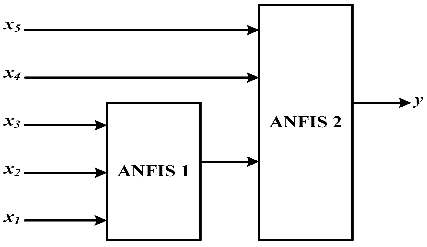
Figure 4.
The wavelet decomposition and reconstruction of a signal.
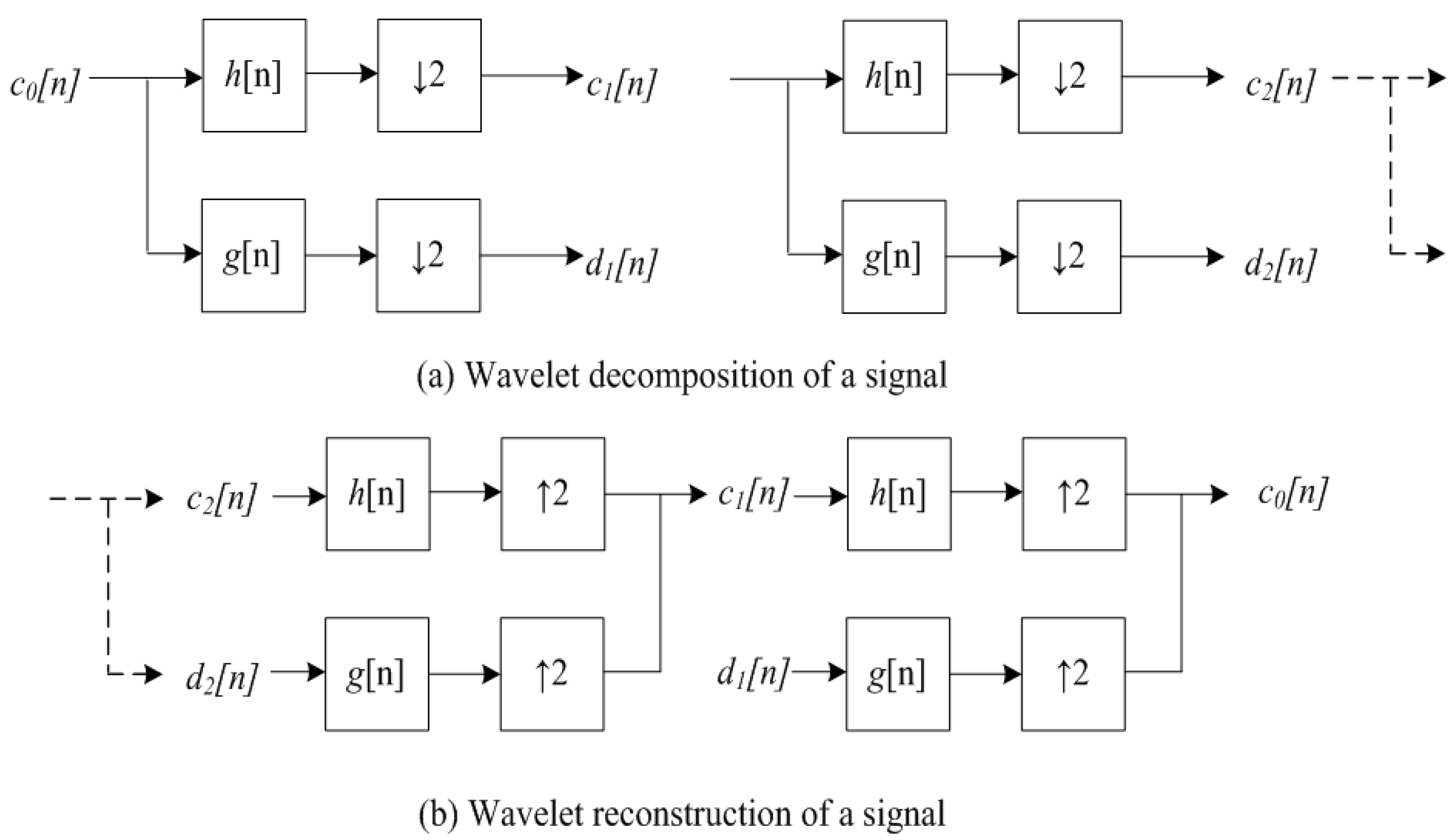
Figure 5.
Pseudo code of the Gravitational Search Algorithm (GSA).

Figure 6.
Pseudo code of the Cuckoo Optimization Algorithm (COA).
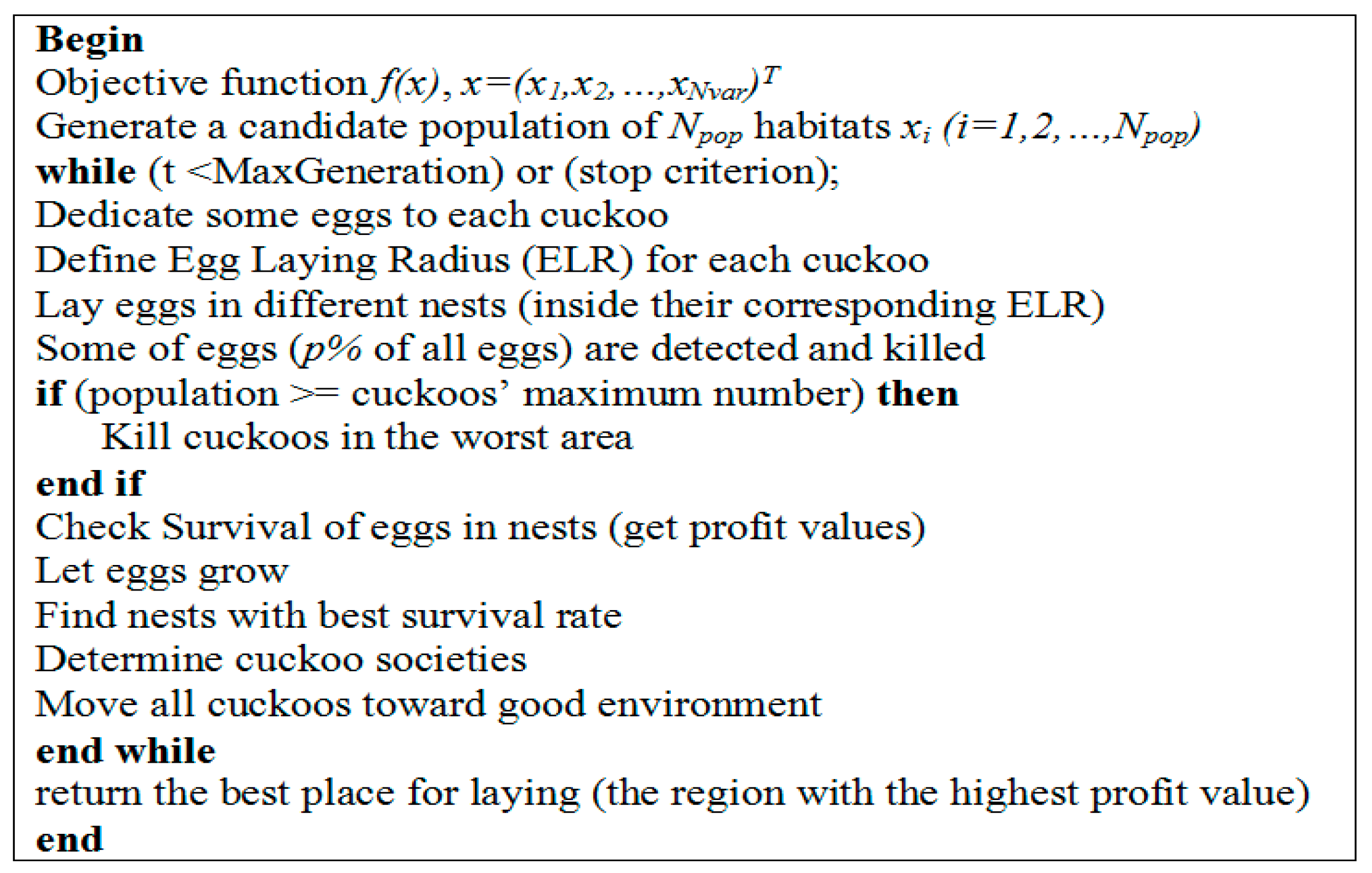
Figure 7.
Pseudo code of the Cuckoo Search (CS).

Figure 8.
Proposed methodology.

Figure 9.
The flowchart of using heuristic algorithms to optimize clustering parameters
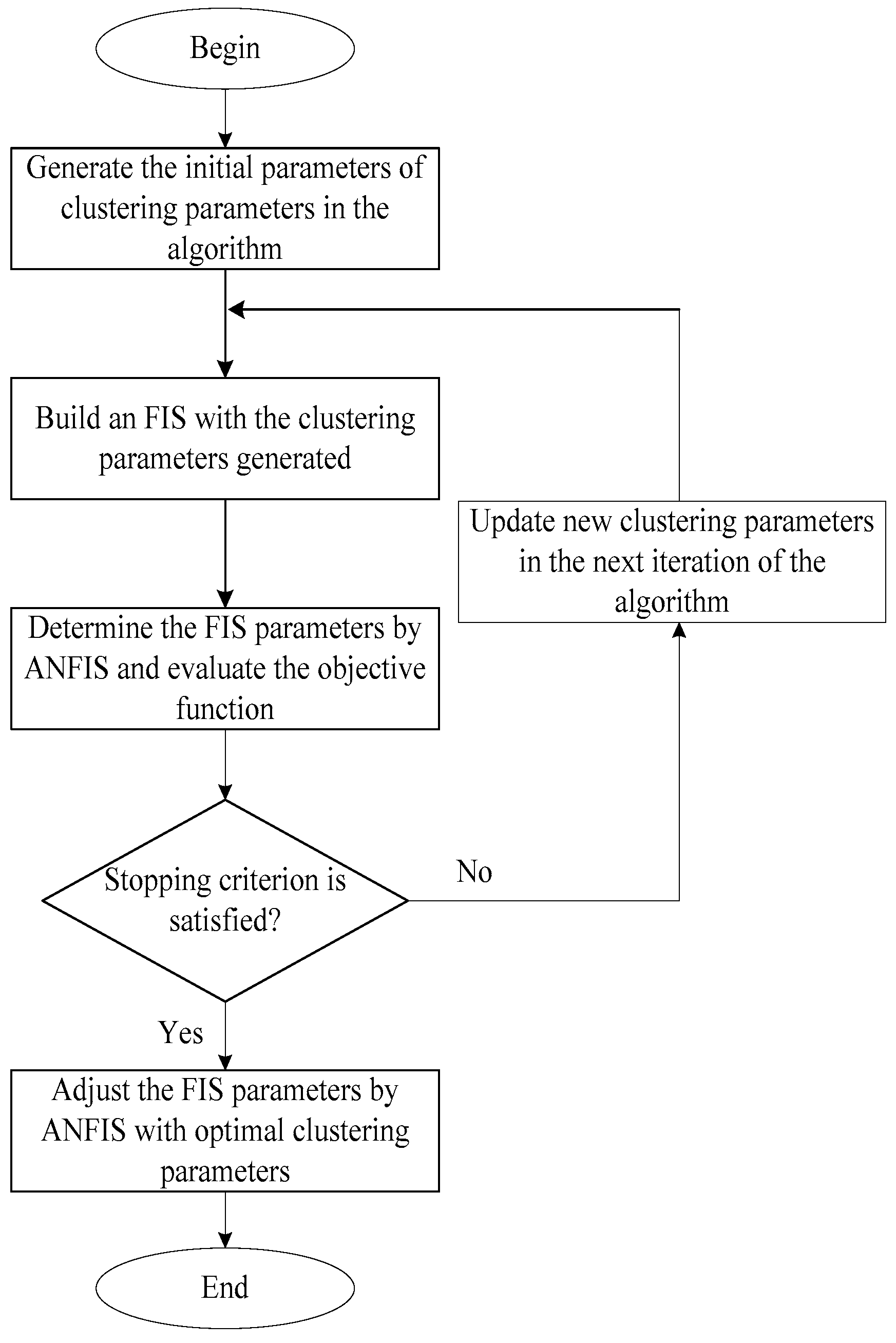
Figure 10.
The hierarchical Adaptive Neuro Fuzzy Inference System (ANFIS) model for forecasting electricity demand.
Figure 10.
The hierarchical Adaptive Neuro Fuzzy Inference System (ANFIS) model for forecasting electricity demand.

Figure 11.
Actual data and forecasting values by artificial neural network (ANN), gravitational search algorithm-hierarchical adaptive neuro-fuzzy inference system (GSA-HANFIS), and wavelet GSA-HANFIS.
Figure 11.
Actual data and forecasting values by artificial neural network (ANN), gravitational search algorithm-hierarchical adaptive neuro-fuzzy inference system (GSA-HANFIS), and wavelet GSA-HANFIS.

Figure 12.
Actual data and forecasting values by ANN, cuckoo optimization algorithm-hierarchical adaptive neuro-fuzzy inference system (COA-HANFIS), and wavelet COA-HANFIS.
Figure 12.
Actual data and forecasting values by ANN, cuckoo optimization algorithm-hierarchical adaptive neuro-fuzzy inference system (COA-HANFIS), and wavelet COA-HANFIS.

Figure 13.
Actual data and forecasting values by ANN, cuckoo search-hierarchical adaptive neuro-fuzzy inference system (CS-HANFIS), and wavelet CS-HANFIS.
Figure 13.
Actual data and forecasting values by ANN, cuckoo search-hierarchical adaptive neuro-fuzzy inference system (CS-HANFIS), and wavelet CS-HANFIS.
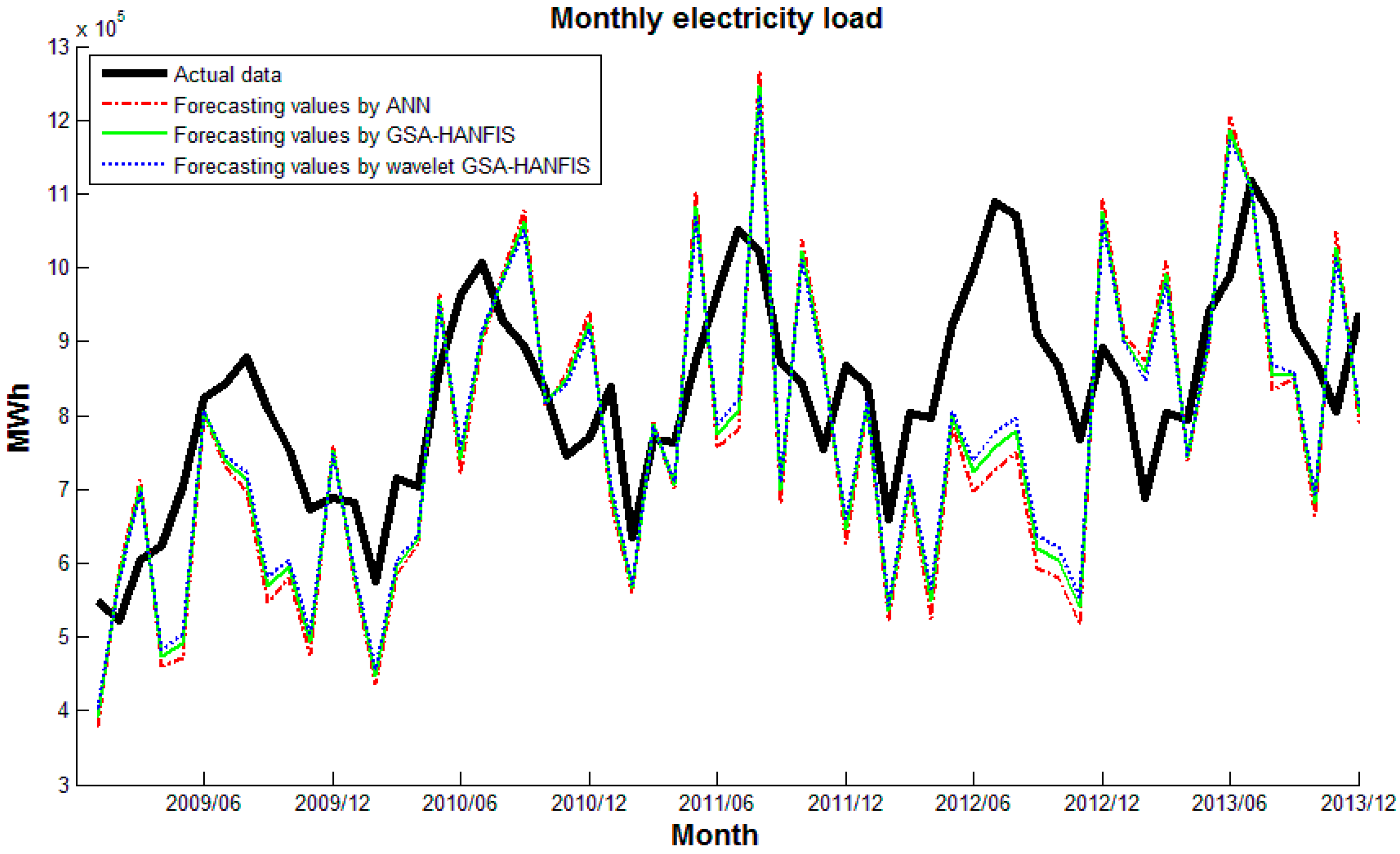

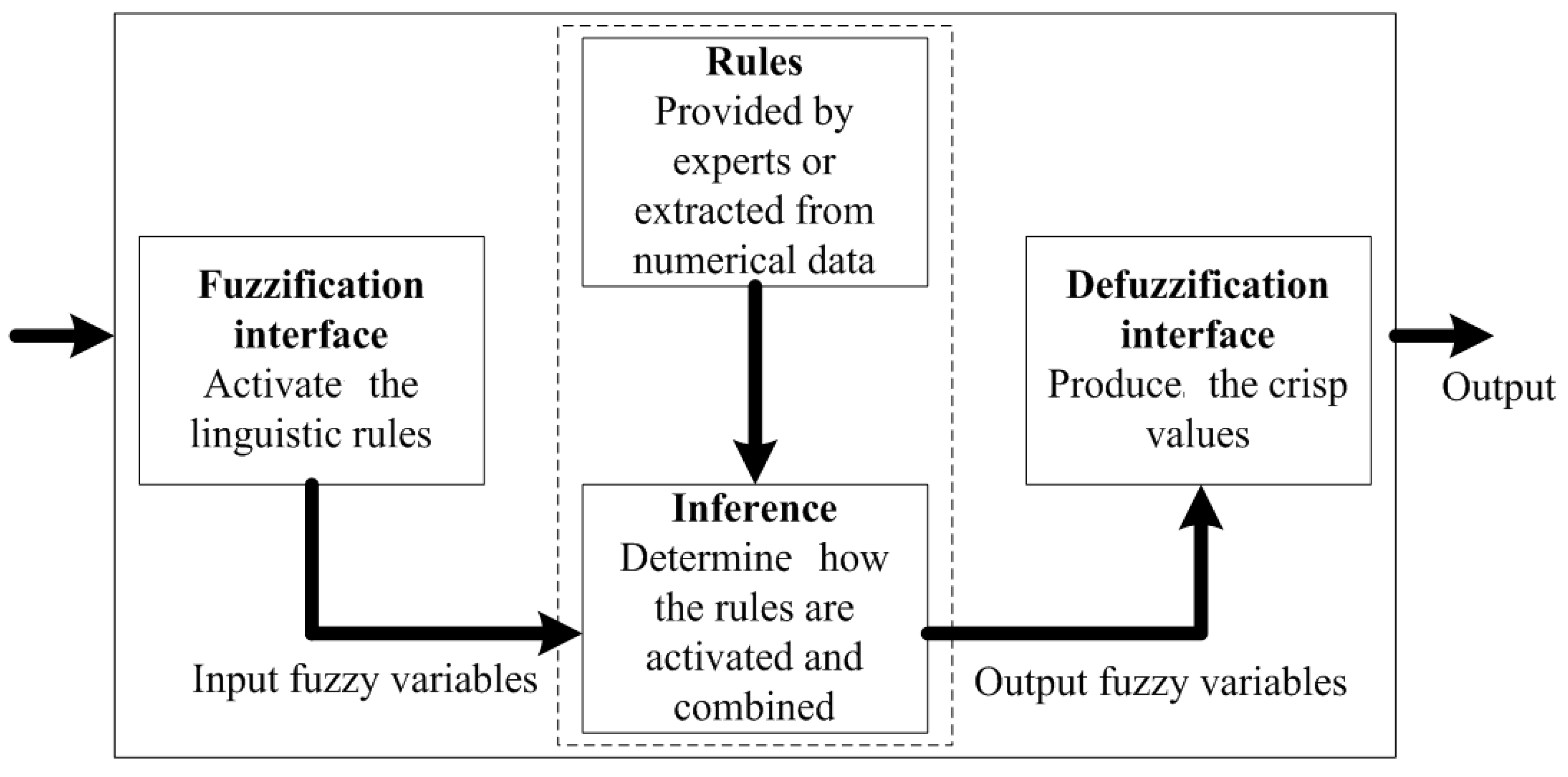
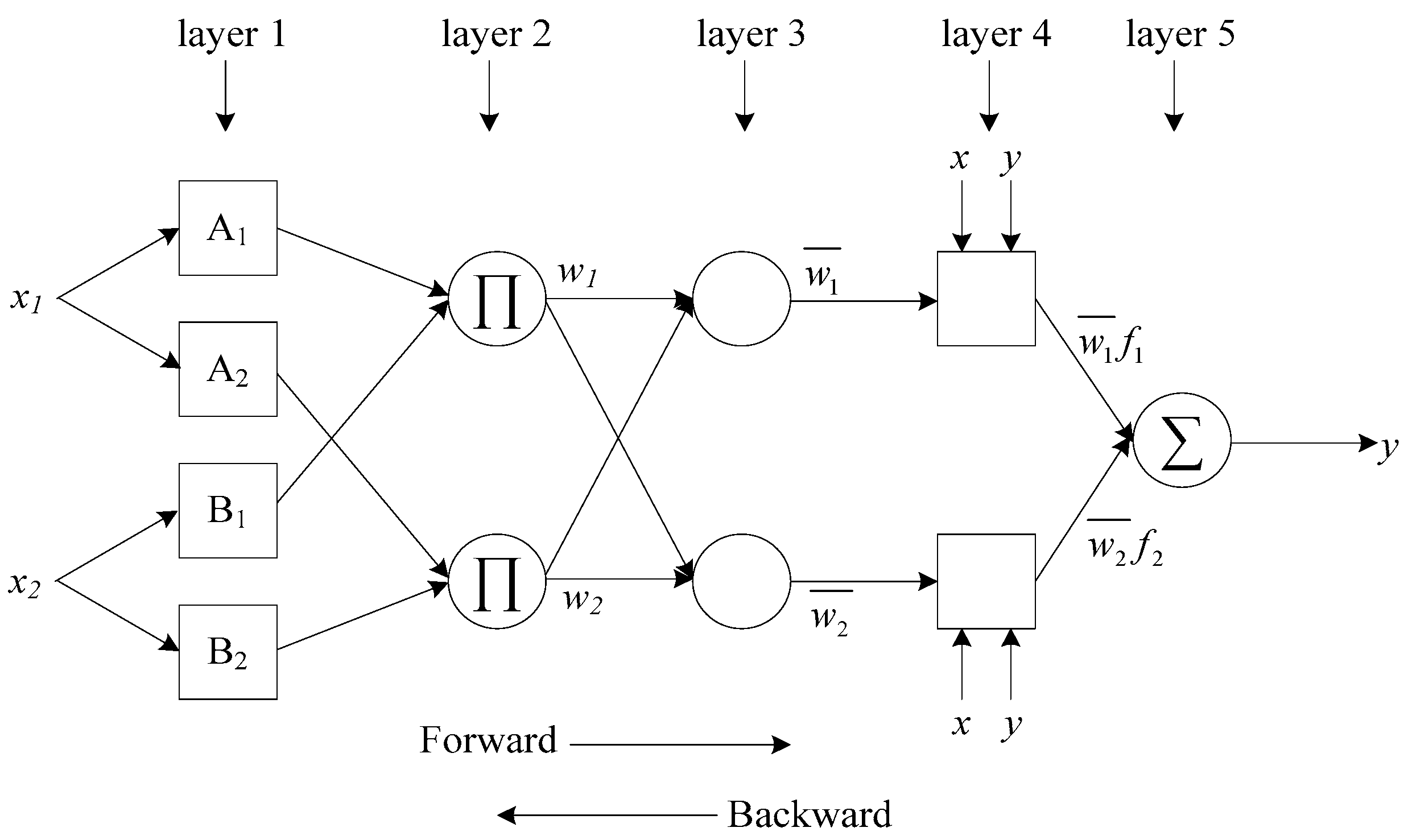
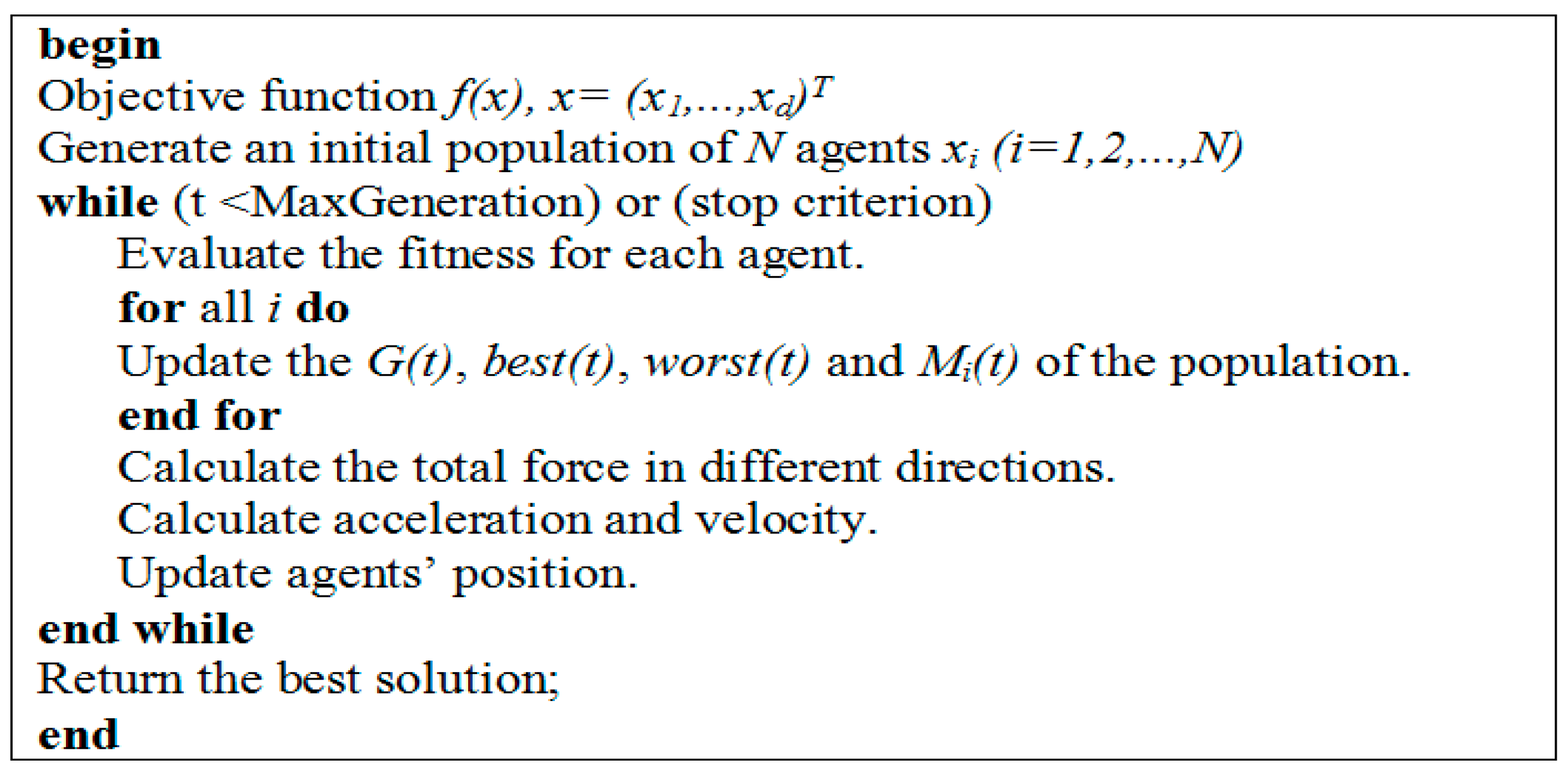
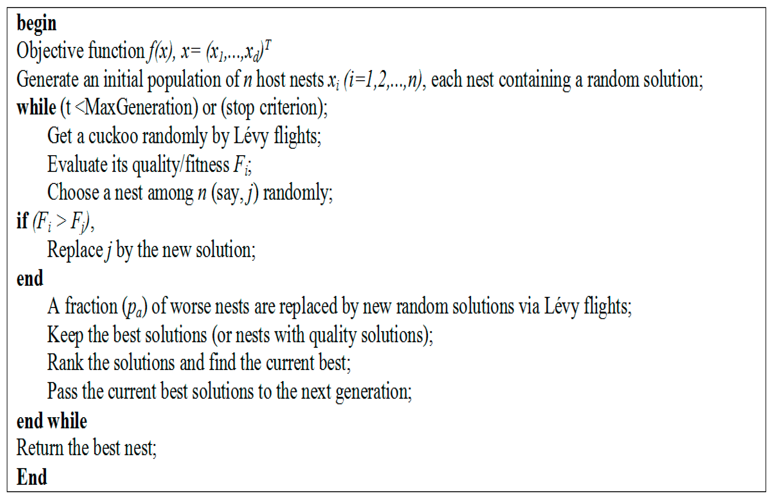
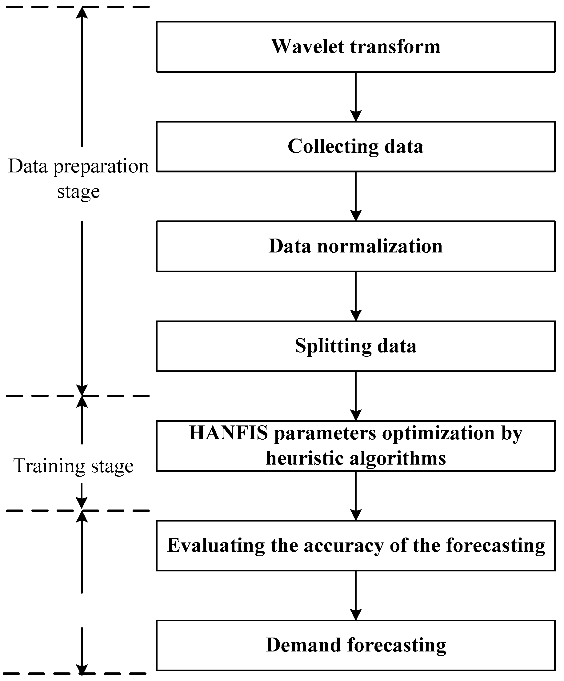
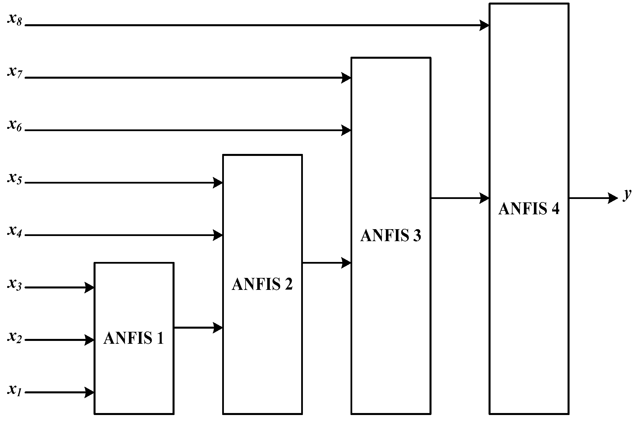
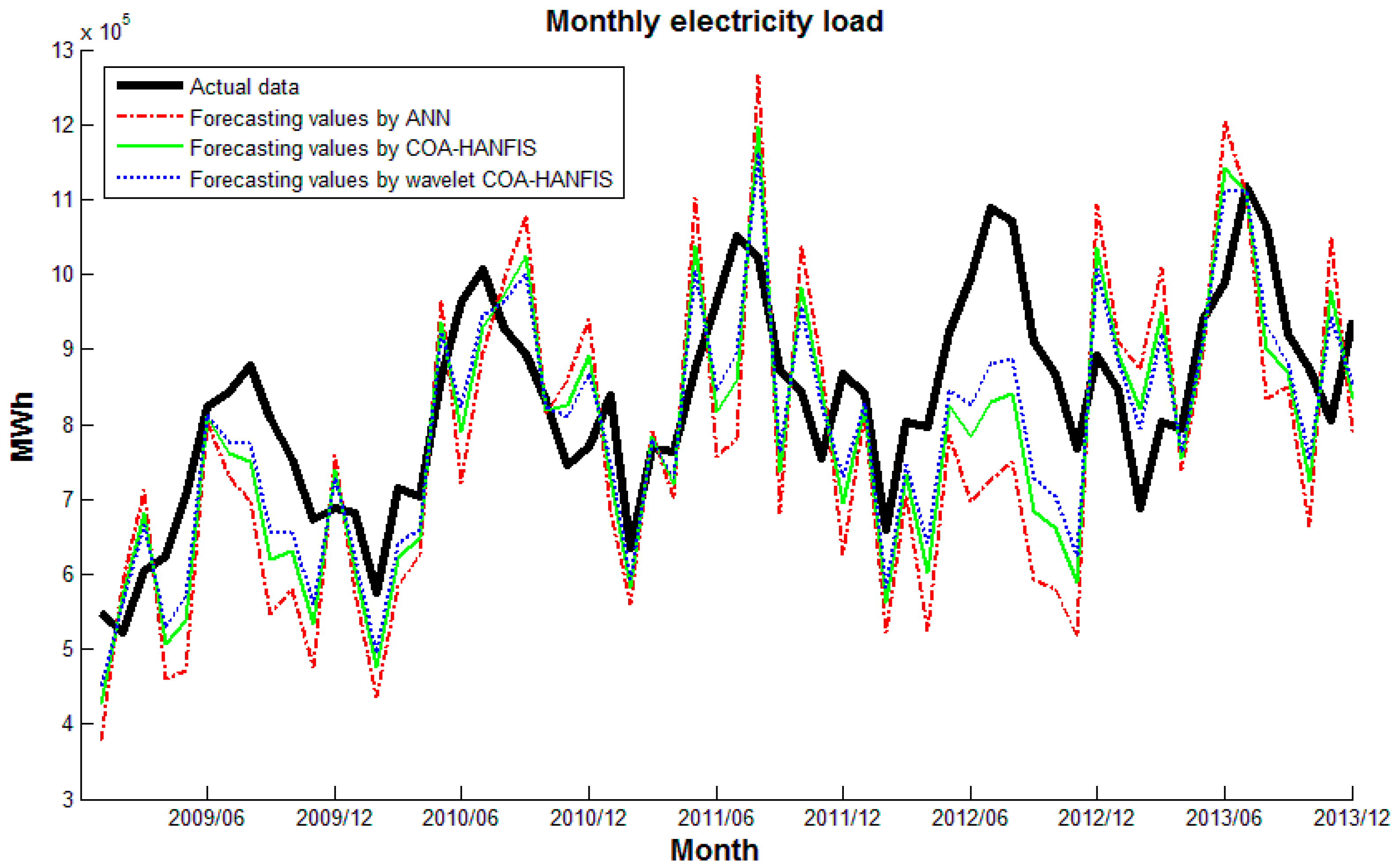
Table 1.
Factors used for electricity forecasting.
| Factor | |
|---|---|
| X1 | Month index |
| X2 | Average air pressure |
| X3 | Average temperature |
| X4 | Average wind velocity |
| X5 | Rainfall |
| X6 | Rainy time |
| X7 | Average relative humidity |
| X8 | Daylight time |
Table 2.
Performance statistics developing models.
| Model | MAPE | RMSE | MAE | R |
|---|---|---|---|---|
| ANN | 0.3953 | 197,234 | 152,084 | 0.5634 |
| GSA-HANFIS | 0.2843 | 183,118 | 123,108 | 0.6142 |
| Wavelet GSA-HANFIS | 0.2023 | 134,126 | 101,321 | 0.7409 |
| COA-HANFIS | 0.0947 | 75,148 | 67,100 | 0.8700 |
| Wavelet COA-HANFIS | 0.0764 | 54,123 | 66,267 | 0.8779 |
| CS-HANFIS | 0.0577 | 47,210 | 60,129 | 0,8934 |
| Wavelet CS-HANFIS | 0.0433 | 39,073 | 49,238 | 0.9287 |
Table 3.
Performance statistics of the autoregressive integrated moving average (ARIMA) and multiple linear regression (MLR).
Table 3.
Performance statistics of the autoregressive integrated moving average (ARIMA) and multiple linear regression (MLR).
| Method | MAPE | RMSE | MAE | R |
|---|---|---|---|---|
| MLR | 0.1702 | 160,540 | 141,870 | 0.6331 |
| ARIMA (2,1,1) | 0.1693 | 152,070 | 136,253 | 0.7146 |
© 2018 by the authors. Licensee MDPI, Basel, Switzerland. This article is an open access article distributed under the terms and conditions of the Creative Commons Attribution (CC BY) license (http://creativecommons.org/licenses/by/4.0/).
Share and Cite
MDPI and ACS Style
Chen, J.-F.; Do, Q.H.; Nguyen, T.V.A.; Doan, T.T.H. Forecasting Monthly Electricity Demands by Wavelet Neuro-Fuzzy System Optimized by Heuristic Algorithms. Information 2018, 9, 51. https://doi.org/10.3390/info9030051
AMA Style
Chen J-F, Do QH, Nguyen TVA, Doan TTH. Forecasting Monthly Electricity Demands by Wavelet Neuro-Fuzzy System Optimized by Heuristic Algorithms. Information. 2018; 9(3):51. https://doi.org/10.3390/info9030051
Chicago/Turabian StyleChen, Jeng-Fung, Quang Hung Do, Thi Van Anh Nguyen, and Thi Thanh Hang Doan. 2018. "Forecasting Monthly Electricity Demands by Wavelet Neuro-Fuzzy System Optimized by Heuristic Algorithms" Information 9, no. 3: 51. https://doi.org/10.3390/info9030051
Note that from the first issue of 2016, this journal uses article numbers instead of page numbers. See further details here.