Residual Recurrent Neural Networks for Learning Sequential Representations


State Key Laboratory of Industrial Control, Zhejiang University, No. 38 Zheda Road, Hangzhou 310000, China
*
Author to whom correspondence should be addressed.
Information 2018, 9(3), 56; https://doi.org/10.3390/info9030056
Submission received: 1 February 2018
/
Revised: 3 March 2018
/
Accepted: 4 March 2018
/
Published: 6 March 2018
Abstract
:Recurrent neural networks (RNN) are efficient in modeling sequences for generation and classification, but their training is obstructed by the vanishing and exploding gradient issues. In this paper, we reformulate the RNN unit to learn the residual functions with reference to the hidden state instead of conventional gated mechanisms such as long short-term memory (LSTM) and the gated recurrent unit (GRU). The residual structure has two main highlights: firstly, it solves the gradient vanishing and exploding issues for large time-distributed scales; secondly, the residual structure promotes the optimizations for backward updates. In the experiments, we apply language modeling, emotion classification and polyphonic modeling to evaluate our layer compared with LSTM and GRU layers. The results show that our layer gives state-of-the-art performance, outperforms LSTM and GRU layers in terms of speed, and supports an accuracy competitive with that of the other methods.
1. Introduction
Recurrent neural networks (RNNs) have proved to be efficient to learn sequential data, such as in acoustic modeling [1,2], natural language process [3,4], machine translation [5,6], and sentiment analysis [7,8]. An RNN is different from other layer structures in hierarchical networks because of its horizontal propagations between the nodes in the same layer. These propagations connect the outputs of RNN [9,10] with the sequence of inputs and past information. With some preprocesses, a RNN is capable of modeling sequences of variable lengths.
However, when the scales of the long-term dependencies to learn are large enough, the RNNs are difficult to train properly. The conventional RNNs are difficult to be trained because of the vanishing gradient and exploding gradient [11,12,13,14]. The gradient issues come from the continuous multiplication in the backpropagation through time (BPTT) [15] with the increasing requirement of learning long-term dependencies. The issues are becoming obvious with the enlargement of the time contributed scale.
To solve the issues, some modified RNN units have been created. A long short-term memory (LSTM) [16] is proposed by Hochreiter and Schmidhuber. Other than a conventional RNN, a LSTM is composed of a memory cell and three gates: an input gate, a forgetting gate and an output gate. The memory cell is updated by partially forgetting the existing memory and adding new memory content. The output layer determines the degree of the memory exposure.
Recently, another gated RNN unit, gated recurrent unit (GRU) [17], has been introduced by Cho et al. in the context of machine translation. Each recurrent unit can adaptively capture dependencies of different time scales. In contrast to an LSTM, a GRU does not have a standalone memory cell and only contains two gates: an update gate, which controls the degree of the unit update, and a reset gate, which controls the amount of the previous state it preserves.
LSTMs and GRUs both use gates to restrain the gradient vanishing and exploding with the cost of being time-consuming and having high computational complexity. In this paper, we introduce a novel recurrent unit with residual error. The residual is first introduced in the residual networks (ResNet) [18,19], which refreshes the top performance in ImageNet database [20]. Residual learning is proven to be effective to restrain vanishing gradient and exploding gradient in the very deep networks [18,19,21]. In the proposed residual recurrent networks (Res-RNN), we use residual learning to solve the gradient issues in the process of horizontal propagation in training. In this paper, we will use theoretical analyses and experiments to prove that the proposed Res-RNN is valid and efficient to modify conventional RNNs.
This paper is organized as follows. In the next section, we will describe the reasons of gradient vanishing and exploding problems and the solutions that have been proposed. This section involves the details of the LSTM and GRU, and why they solve the gradient issues. In the third section, we propose our Res-RNN unit and analyze how residual learning helps to train the RNNs. The fourth section demonstrates the results of our network and then compares the results with simple RNN, LSTM and GRU in various fields: airline travel information system (ATIS) database [22], Internet movie database (IMDB) [23] and polyphonic database [24]. The experiments show that our novel recurrent unit can provide state-of-the-art performance.
2. Recurrent Neural Networks and Its Training
2.1. Gradient Issues
It is well known that the training of RNNs is difficult when learning long-term dependencies [14]. A common approach of updating gradient in training is backpropagation through time (BPTT). The recurrent model can be unfolded as a multi-layer one with connections to the same layer, and backpropagation through time is similar to the backpropagations in other hierarchical networks, such as deep brief networks (DBN), auto-encoder (AE) and convolutional neural networks (CNN). A generic RNN, with an input and the state is given by
where is the collection of the input weight matrix , recurrent weight matrix and the bias . In details, the state at the timestamp is described as
where σ is the sigmoid function. Denoting the cost function as , the BPTT is formulated as
where is the time distributed length. As Bengio et al. [11,12,13] discussed and Equation (5) shows, the gradient issues are relative to the continuous multiplications. Because of long-term states, the gradient exploding happens when the gradient grows exponentially, while the gradient vanishing happens when the gradient goes exponentially quickly to norm 0. Both the issues stop the model from updating itself.
Initial solutions to RNN gradient issues focus on training, such as in weight decays and more efficient optimization methods [14]. Then, LSTMs and GRUs exploit gates to reformulate the state. LSTMs use three gates and a memory cell to reformulate the RNNs. The details of LSTMs are computed as
where , and represent the input, forget and output gates, respectively. is the internal memory of the unit. is a candidate hidden state that is computed based on the current input and the previous hidden state. is the sigmoid function and means the element-wise multiplication. The details of GRUs are described as
where r and z is the reset gate and the update gate, respectively. The structures of the RNN, LSTM and GRU are shown in Figure 1. The gate functions, such as , and in an LSTM, restrain the exploding of memory gradient and reformulate the gradient from a continuous multiplication expression to a sum expression. That is why LSTMs and GRUs can solve the problem issues, especially the vanishing gradient.
2.2. Residual Learning and Identity Mapping
Residual learning is used to learn the residual function with reference to the direct hidden state instead of unreferenced functions. Residuals have recently achieved successes in very deep CNNs for image recognition and objection detection [18,21]. He et al. use a Res-Net [18] to update the top accuracy of ImageNet test, and the Res-Net is composed of residuals and short cuts. Szegedy et al. [21] introduce the residual-shortcut structure to improve GoogLeNet [25,26,27] and propose the Inception-V4 [21]. Residual representations are widely used in the image recognition. The Vector of Aggregate Locally Descriptor (VLAD) Vector of Aggregate Locally Descriptor [28] and Fisher vector [29] is representations for image features. The encoder residual vectors [30] are more effective than encoding original vectors.
In the sequence and video learning, the results strongly rely on the inputs and the differences between states. The residual learning depends on variables that represent residual vectors between two segments of a long sequence. It has been experimentally proved that the residual learning continues converging in deep networks and long-term RNN. It suggests that the reformulation with residual functions can make the optimization of the weights easy and promote the performance of RNNs.
Shortcut connections have been a hot topic for a long time. The original model of shortcut connections is used to add linear connections between the inputs and the outputs [31,32,33]. Successive modifications focus on adding gates to determine the degree of shortcut connection. There also exist gradient issues in very deep hierarchical networks. The shortcut structure is proven to be easier to be optimized and achieves higher accuracy by considerably increasing depth. Highway Networks [34] construct shortcuts by gate functions to increase the depth. He et al. [18,19] introduce the residual-shortcut structure to build a deep networks with a depth of 152 layers. The identity mapping can propagate the information completely to the next node, including the gradients. The residual learning and shortcut connections are useful to solve the exploding and vanishing gradient problems in long-term backpropagation.
3. Residual Recurrent Neural Network
3.1. Residual-Shortcut Structure
In this section, we introduce the residual error into a RNN layer: residual recurrent neural networks (Res-RNN). This Res-RNN layer learns the residual functions with reference to the direct hidden state instead of unreferenced functions.
Given a conventional RNN unit at the timestamp , the current state is calculated by the last state and the input, as
where is the hypothesis of the input , is the state-to-state weight matrix, is the activation function. The hypothesis is expressed by
where is the input-to-state weight matrix, and is the bias vector. The output of RNN can be used for classification and prediction of the next term.
As is an underlying mapping from state to state, we learn this mapping with a residual, given by
Thus, the state is calculated as
Equation (11) is composed of a shortcut connection and an element-wise addition. The shortcut connection does not introduce extra parameters and computation complexity. This reconstruction makes the loss function approximate to an identity mapping. When the recurrent connections are formulated as identity mapping, the training error should be non-increasing. To drive Equation (11) to approach an identity mapping, the weights of nonlinear block in Equation (11) are tuned towards zero.
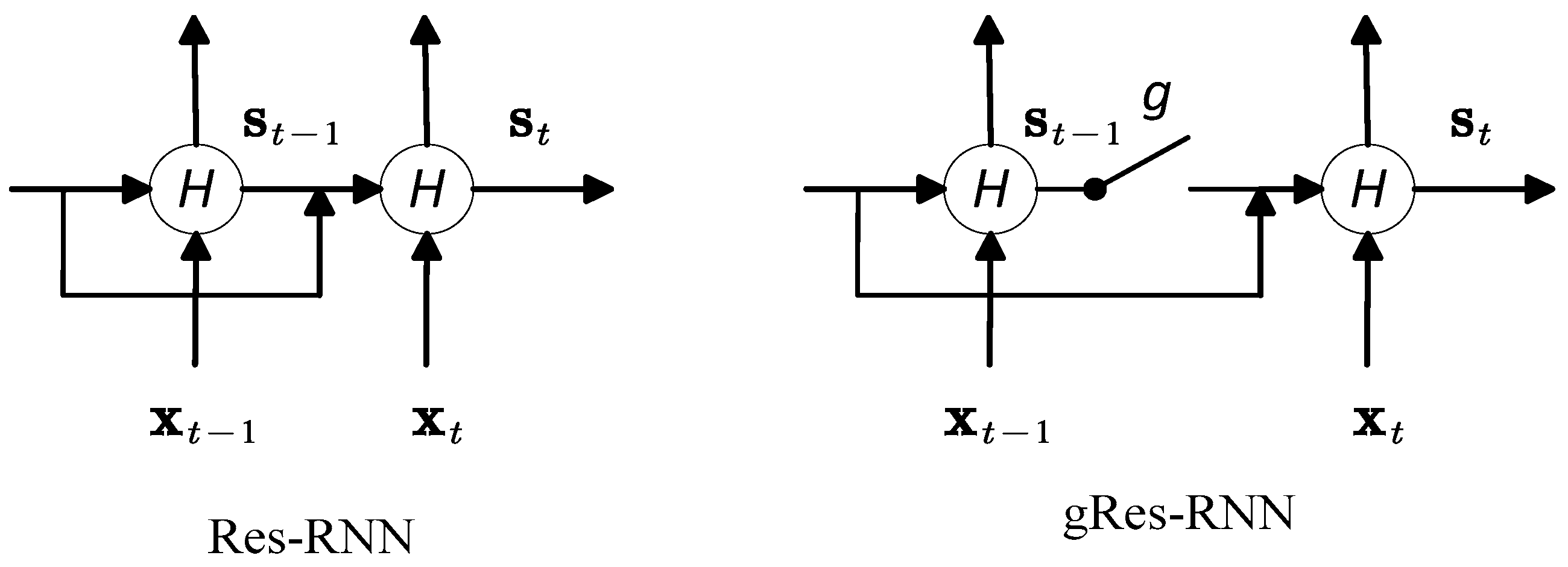
Considering the dimension equation, a linear projection is introduced to match the dimensions. Thus, the forward propagation of Res-RNN is shown as
where is the residual function, is the linear projection weight. is the non-linear activation function and an identity mapping. There exist two identity mappings in Res-RNN layer, and . They are the necessary connections, and their impacts will be discussed in the next section.
Furthermore, we try to add a linear gate to determine the input of the residual with W, so that the Equation (12) is reconstructed as
or a gate function such as the LSTM and GRU as
where
The experiments show that the gate function helps to improve the performance with increasingly small calculation complexity. Besides this, in practice, the batch normalization for RNNs [35] is introduced to the hidden-to-hidden transition to reduce the covariate shift between time steps. It helps the network achieve faster convergence and better generalization. The structure of our Res-RNN is described in Figure 2.
3.2. Analysis of Res-RNN
As discussed, the state is the addition of an identity mapping and a residual function. The activation function is also an identity mapping. For the reason of recurrent transmission and the residual learning as Equation (11), the state can be unrolled as
where is the length of sequential dependencies. The accumulation equation (Equation (17)) shows that any state can be represented as a former state and a sum of residuals. When the initial state is 0, the state of timestamp is the sum of series of residuals.
Equation (17) results in a better backward propagation. Considering the loss function represented in Equations (7)–(9), with the residual accumulation in the Equation (17), the gradient in BPTT is
Equation (18) describes that the gradient can be decomposed into two additive parts. One is , which propagates information directly without weights, the other is the accumulation, , which needs the inner product with weight matrices. The direct propagation part ensures the gradient information can be propagated to any state. The direct gradient part comes from the two identity mappings. It suggests that the information can be entirely propagated both forward and backward, even when the weights are arbitrarily small. As the accumulation part, , cannot always be −1, the gradient of a state does not vanish through BPTT in a mini-batch.
Moreover, we introduce gate functions into the Res-RNN, which is known as gated Res-RNN (gRes-RNN). The gRes-RNN adds a gate function to the residual part. The gradient of gate function is describe as
The gate function transforms the gradient into a sum expression instead of continuous multiplication, which avoids the gradient issues. Besides, the gated function is trained and activated. The activation function can regularize the residuals in a “good” range, and the training can learn to control the exposure degree of residuals.
4. Experiments and Discussion
In this part, we use various tasks and databases to show the performance and compare the results with other RNN units. The databases are respectively the ATIS database [22], IMDB database [23] and Polyphonic music database [24]. These databases can evaluate the performance of sequence learning, emotion classification and polyphonic music modeling. Our results will be compared with the RNN, LSTM, and GRU. In the experiments, we choose the RMSProp as the optimizer method for background propagation. The experiments are done on NVIDIA GTX970 and programed by Tensorflow. Our experiments are done as follows: (1) the datasets are divided into three parts: training set, validation set and testing set; (2) the best model is saved according to the best validation performances, and the test performances are given by the best models; (3) the results are averaged over the repetitions with the same model parameters but different random seeds for initialization of the weights.
4.1. ATIS Database
The ATIS (airline travel information system) database [22] is a database collected by the Defense Advanced Research Projects Agency (DARPA). It is represented by Inside Outside Beginning (IOB). The ATIS official split contains 4978/893 sentences for a total of 56,590/9198 words (average sentence length is 15) in the train/test set. It is used to train for spoken language understanding.
The models are composed of a variable-size input layer adaptive with the input size, a word-embedding layer with the output dimension of 100, a recurrent layer returning sequences and a time-distributed dense layer activated by for classification. We set the number of the hidden units as 100 and the activation function of recurrent layer as , and train the models for 100 epochs. We take 3000 samples from the dataset for training, 1000 for validation and 1000 for testing. The model checkpoint is set to save the best model weights when achieving the best valid F1. The learning rate is 0.01 so that the model is steady before 100 epochs [36]. The performances of the best models are measured by the conlleval PERL script and the experimental results are shown as follows.
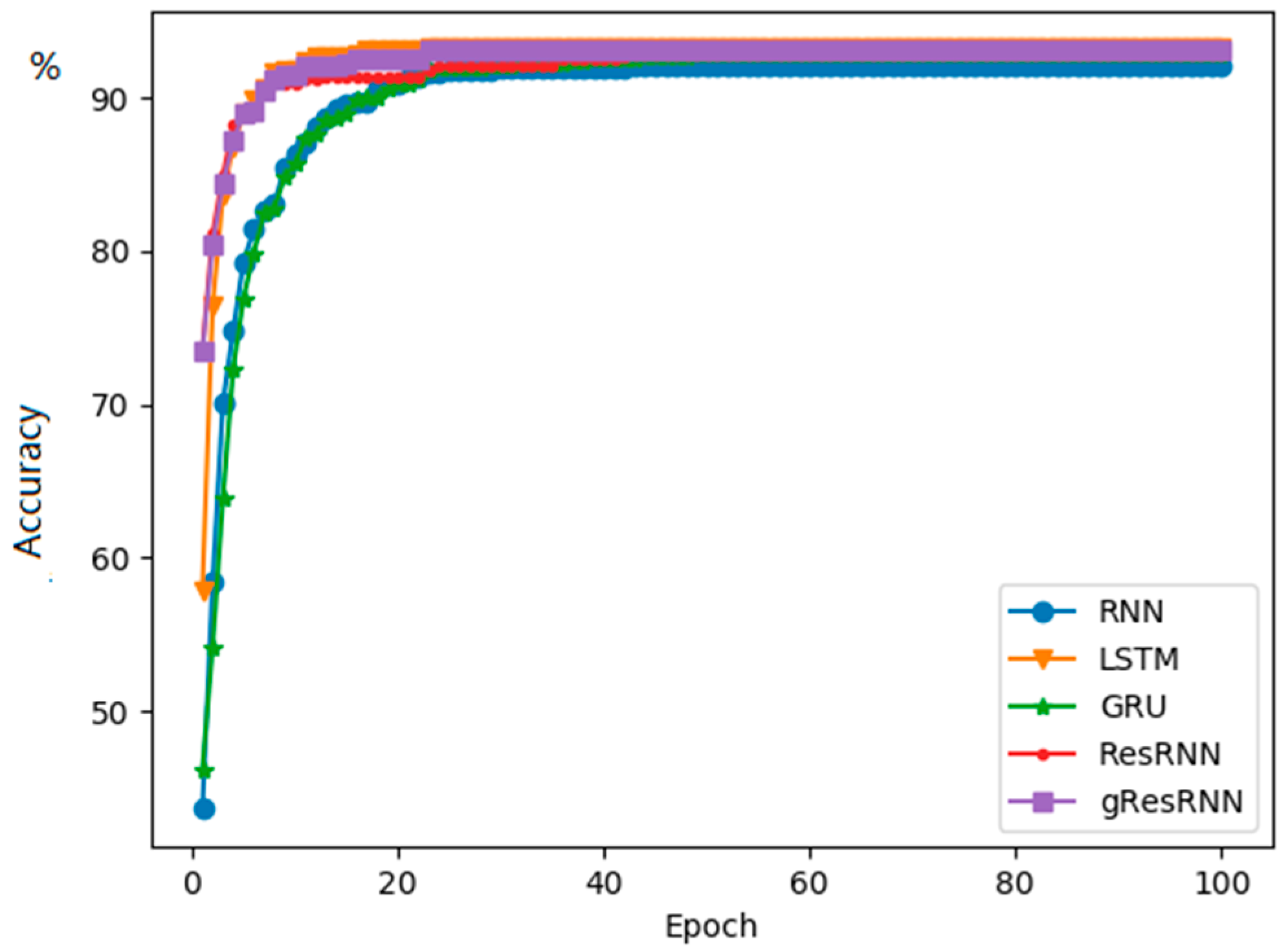
From Table 1, it is clear that the LSTM achieves the best accuracy. Our results provide a competitive accuracy with LSTM in this task of spoken language understanding, but better than the RNN and GRU. On the aspect of time consumption, the Res-RNN only takes approximately half of the time in training than the LSTM and GRU. Even the gated Res-RNN takes significantly less time than the GRU and LSTM. The testing results do not perform as well as training and validation because we do not add a dropout layer before the last dense layer. Figure 3 shows the best F1 updates of the models. It shows that our models are trained faster than the GRU and RNN in this experiment. Besides this, after approximately 30 epochs, the best F1 of other models stays the same, but our model can update the best F1 score even after 100 epochs, even though the update is very small and hard to show in the figure. It indicates that our model is easy to be optimized for a better performance.
4.2. IMDB Database
The Internet movie database (IMDB) database (large movie review dataset) [23] is a dataset for binary sentiment classification containing substantially more data than previous benchmark datasets. It provides a set of 25,000 highly polar movie reviews for training, and 25,000 for testing. Each review contains tens of words. It is used to train for sentiment analysis.
The models are composed of a variable-size input layer adaptive with the input size, a 64-dimensional word-embedding layer, a recurrent layer returning the last state and a dense layer for binary classification. We set the number of the hidden units as 128 and the activation function of recurrent layer as tanh. To show the losses decrease with epoch, we train the models with a small learning rate, , for 10,000 iterations [37].
Table 2 shows the performance of several recurrent networks on the IMDB database. Our Res-RNN takes dramatically less time than GRU and LSTM per epoch. The accuracy of the Res-RNN is close to the performances of the LSTM and GRU.
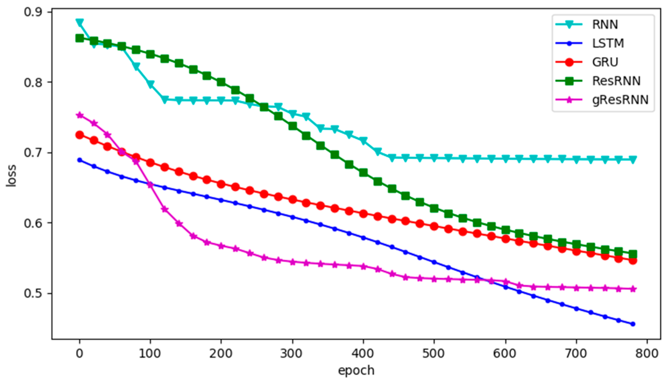
The losses of different networks are shown in Figure 4. In this experiment, the GRU and LSTM converge faster than Res-RNNs, but the Res-RNNs take less time in each epoch. The gated Res-RNN performs better than GRU, but not as well as LSTM. This experiment shows that our Res-RNNs can provide a competitive accuracy with the GRU and LSTM with less training and testing time.
4.3. Polyphonic Databases
There exist four polyphonic music databases [24]: Nottingham, Muse data, JSB chorales and piano-midi. They are used to train the polyphonic music model and generate new music from the model. The models are composed of a 16-dimensinal input layer, a 64-dimensional word-embedding layer, a recurrent layer returning the sequence and a dense layer for 88-dimensional classification. We set the number of the hidden units as 128 and the activation function of recurrent layer as tanh, training the models with the loss function of categorical cross entropy for 10,000 epochs [38]. The learning rate is set as to show the decreases of the losses decrease with epoch. This experiment is used to evaluate the performance of generalization and the speed of convergence.
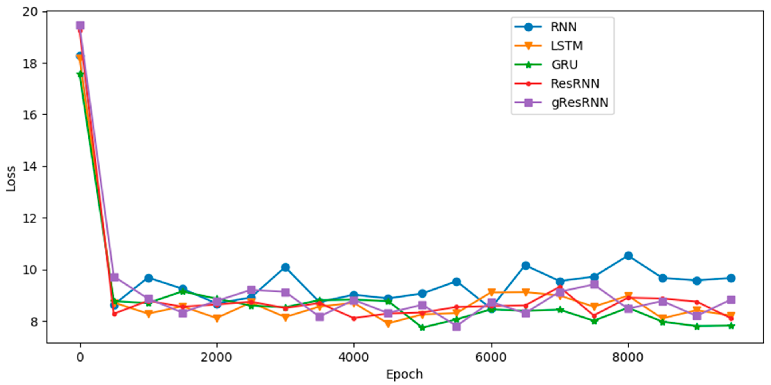
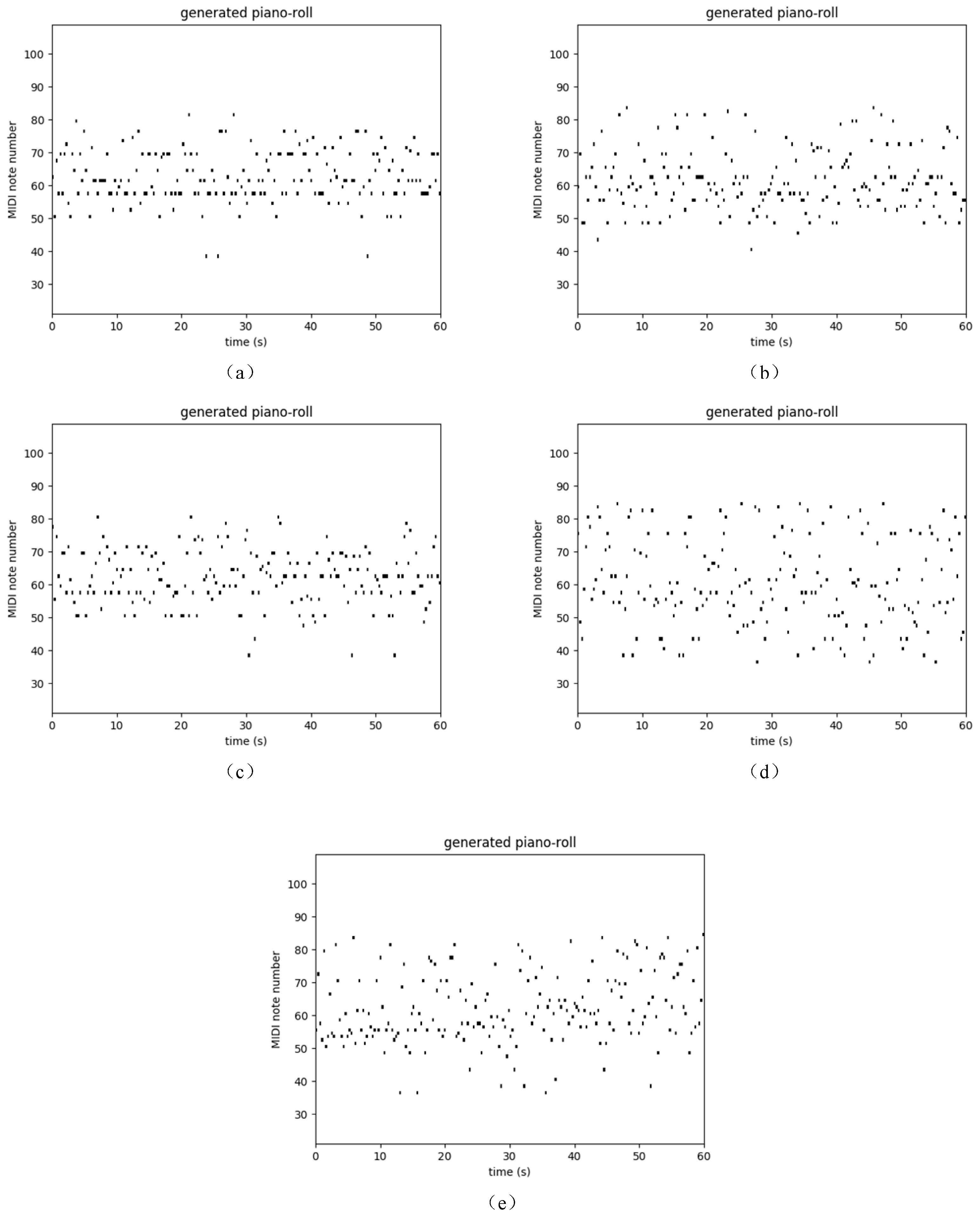
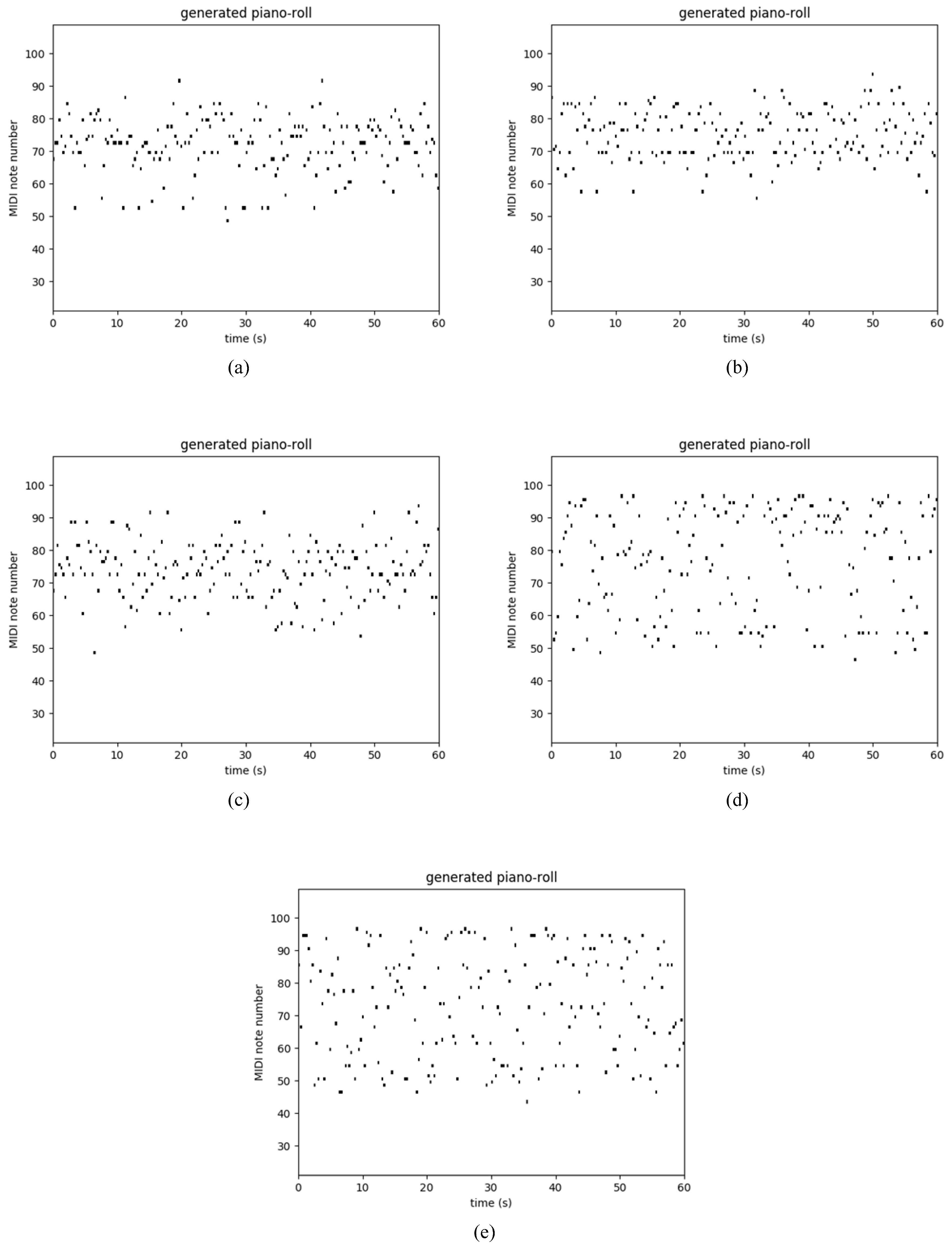
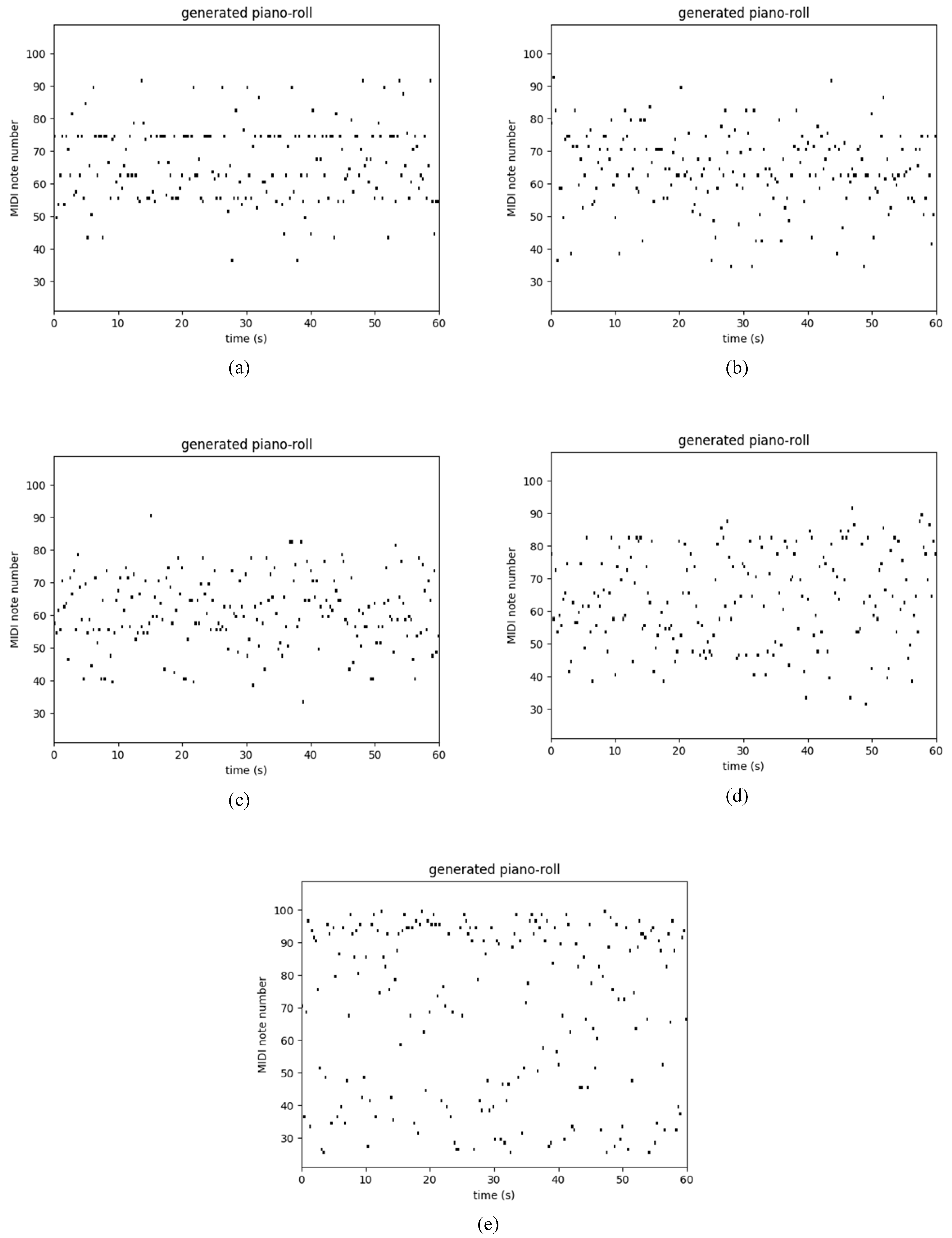
Table 3 shows the performance of several recurrent networks on the polyphonic music databases. As usual, our Res-RNNs take dramatically less time than the GRU and LSTM per epoch. The losses of our Res-RNNs are close to the GRU and LSTM. In some of the databases, the Res-RNN performs better than the LSTM and GRU with time. The loss decreases are shown in the Figure 5. Figure 5 shows that our Res-RNNs support a state-of-the-art result with the LSTM and GRU. To testify the generalization ability of different networks, we create a random sequence as the seed to generate entire music, and Figure 6, Figure 7, Figure 8 and Figure 9 show the results by learning from different database, in which y axis represents the notes and x axis shows the timestamps. Figure 6, Figure 7, Figure 8 and Figure 9 show that our models generate music with the notes distributed sparse, compared with that the RNN generates music with many slices of the same note. Our models support a competitive generalization with the LSTM and GRU, and better than RNN.
5. Conclusions
This paper proposes the Res-RNN, a recurrent neural network with residual learning and shortcut connections. A key feature of our layer is that, other than gate functions, we introduce a novel solution—residual learning—to solve the exploding and vanishing gradient. The residual and shortcut structure change the mapping to an identity one which can propagate the gradients perfectly. The experiments show the performance of our modeling on sequence prediction, classification and generation. The first experiment with the ATIS dataset evaluates the performance on the sequence prediction. The Res-RNNs performs better than the RNN and GRU, but a little worse than LSTM. The second experiment with the IMDB database evaluates the performance on the sequence classification. With enough epochs, the Res-RNNs can achieve a satisfying result in classification. The last experiment with polyphonic music databases shows the Res-RNNs can achieve as good results as the LSTM and GRU. In all the experiments, the Res-RNNs are obviously faster than the LSTM and GRU. The experiments show that the Res-RNNs can solve the vanishing and exploding gradient issues with a remarkable improvement in training and predicting speed.
In addition to the experiments referred, our sequence model has the capability for multi-dimension data, including but not limited to video prediction. Further research is coming soon.
Acknowledgments
This research is supported by the National Natural Science Foundation of China (U1664264, U1509203, 61174114).
Author Contributions
Boxuan Yue conceived and designed the experiments; Boxuan Yue performed the experiments; Boxuan Yue and Junwei Fu analyzed the data; Jun Liang contributed guidance and advices; Boxuan Yue wrote the paper.
Conflicts of Interest
The authors declare no conflict of interest.
References
- Hinton, G.; Deng, L.; Yu, D.; Dahl, G.E.; Mohamed, A.; Jaitly, N.; Senior, A.; Vanhoucke, V.; Nguyen, P.; Sainath, T.N. Deep neural networks for acoustic modeling in speech recognition: The shared views of four research groups. IEEE Signal Process. Mag. 2012, 29, 82–97. [Google Scholar] [CrossRef]
- Mohamed, A.; Dahl, G.E.; Hinton, G. Acoustic modeling using deep belief networks. IEEE Trans. Audio Speech Lang. Process. 2012, 20, 14–22. [Google Scholar] [CrossRef]
- Jackson, R.G.; Patel, R.; Jayatilleke, N.; Kolliakou, A.; Ball, M.; Gorrell, G.; Roberts, A.; Dobson, R.J.; Stewart, R. Natural language processing to extract symptoms of severe mental illness from clinical text: The clinical record interactive search comprehensive data extraction (cris-code) project. BMJ Open 2017, 7, e012012. [Google Scholar] [CrossRef] [PubMed]
- Swartz, J.; Koziatek, C.; Theobald, J.; Smith, S.; Iturrate, E. Creation of a simple natural language processing tool to support an imaging utilization quality dashboard. Int. J. Med. Inform. 2017, 101, 93–99. [Google Scholar] [CrossRef] [PubMed]
- Sawaf, H. Automatic Machine Translation Using User Feedback. U.S. Patent US20150248457, 3 September 2015. [Google Scholar]
- Sonoo, S.; Sumita, K. Machine Translation Apparatus, Machine Translation Method and Computer Program Product. U.S. Patent US20170091177A1, 30 March 2017. [Google Scholar]
- Gallos, L.K.; Potiguar, F.Q.; Andrade, J.S., Jr.; Makse, H.A. Imdb network revisited: Unveiling fractal and modular properties from a typical small-world network. PLoS ONE 2013, 8, e66443. [Google Scholar] [CrossRef]
- Oghina, A.; Breuss, M.; Tsagkias, M.; Rijke, M.D. Predicting imdb movie ratings using social media. In Advances in Information Retrieval, Proceedings of the European Conference on IR Research, ECIR 2012, Barcelona, Spain, 1–5 April 2012; Springer: Berlin/Heidelberg, Germany, 2012; pp. 503–507. [Google Scholar]
- Elman, J.L. Finding structure in time. Cogn. Sci. 1990, 14, 179–211. [Google Scholar] [CrossRef]
- Jordan, M.I. Serial Order: A Parallel Distributed Processing Approach; University of California: Berkeley, CA, USA, 1986; Volume 121, p. 64. [Google Scholar]
- Bengio, Y.; Boulanger-Lewandowski, N.; Pascanu, R. Advances in optimizing recurrent networks. In Proceedings of the IEEE International Conference on Acoustics, Speech and Signal Processing, Kyoto, Japan, 25–30 March 2012; pp. 8624–8628. [Google Scholar]
- Bengio, Y.; Frasconi, P.; Simard, P. The problem of learning long-term dependencies in recurrent networks. In Proceedings of the IEEE International Conference on Neural Networks, San Francisco, CA, USA, 28 March–1 April 1993; Volume 1183, pp. 1183–1188. [Google Scholar]
- Bengio, Y.; Simard, P.; Frasconi, P. Learning long-term dependencies with gradient descent is difficult. IEEE Trans. Neural Netw. 1994, 5, 157–166. [Google Scholar] [CrossRef] [PubMed]
- Gustavsson, A.; Magnuson, A.; Blomberg, B.; Andersson, M.; Halfvarson, J.; Tysk, C. On the difficulty of training recurrent neural networks. Comput. Sci. 2013, 52, 337–345. [Google Scholar]
- Sutskever, I. Training Recurrent Neural Networks. Ph.D. Thesis, University of Toronto, Toronto, ON, Canada, 2013. [Google Scholar]
- Sepp, H.; Schmidhuber, J. Long short-term memory. Neural Comput. 1997, 9, 16. [Google Scholar]
- Cho, K.; Merrienboer, B.V.; Gulcehre, C.; Bahdanau, D.; Bougares, F.; Schwenk, H.; Bengio, Y. Learning phrase representations using rnn encoder-decoder for statistical machine translation. arXiv, 2014; arXiv:1406.1078. [Google Scholar]
- He, K.; Zhang, X.; Ren, S.; Sun, J. Deep residual learning for image recognition. In Proceedings of the Computer Vision and Pattern Recognition, Caesars Palace, NE, USA, 26 June–1 July 2016; pp. 770–778. [Google Scholar]
- He, K.; Zhang, X.; Ren, S.; Sun, J. Identity mappings in deep residual networks. In Proceedings of the European Conference on Computer Vision, Amsterdam, The Netherlands, 11–14 October 2016. [Google Scholar]
- Russakovsky, O.; Deng, J.; Su, H.; Krause, J.; Satheesh, S.; Ma, S.; Huang, Z.; Karpathy, A.; Khosla, A.; Bernstein, M. Imagenet large scale visual recognition challenge. Int. J. Comput. Vis. 2015, 115, 211–252. [Google Scholar] [CrossRef]
- Szegedy, C.; Ioffe, S.; Vanhoucke, V.; Alemi, A. Inception-v4, inception-resnet and the impact of residual connections on learning. In Proceedings of the Thirty-First AAAI Conference on Artificial Intelligence, San Francisco, CA, USA, 4–9 February 2017; p. 12. [Google Scholar]
- Price, P.J. Evaluation of spoken language systems: The atis domain. In Proceedings of the Workshop on Speech and Natural Language, Harriman, NY, USA, 23–26 February 1992; pp. 91–95. [Google Scholar]
- Lindsay, E.B. The internet movie database (imdb). Electron. Resour. Rev. 1999, 3, 56–57. [Google Scholar]
- Chung, J.; Gulcehre, C.; Cho, K.H.; Bengio, Y. Empirical evaluation of gated recurrent neural networks on sequence modeling. arXiv, 2014; arXiv:1412.3555. [Google Scholar]
- Ioffe, S.; Szegedy, C. Batch normalization: Accelerating deep network training by reducing internal covariate shift. In Proceedings of the 32nd International Conference on Machine Learning, Lille, France, 7–9 July 2015; pp. 448–456. [Google Scholar]
- Szegedy, C.; Liu, W.; Jia, Y.; Sermanet, P.; Reed, S.; Anguelov, D.; Erhan, D.; Vanhoucke, V.; Rabinovich, A. Going deeper with convolutions. In Proceedings of the 2015 IEEE Conference on Computer Vision and Pattern Recognition (CVPR), Boston, MA, USA, 7–12 June 2015; pp. 1–9. [Google Scholar]
- Szegedy, C.; Vanhoucke, V.; Ioffe, S.; Shlens, J.; Wojna, Z. Rethinking the inception architecture for computer vision. In Proceedings of the IEEE Conference on Computer Vision and Pattern Recognition, Seattle, WA, USA, 27–30 June 2016; pp. 2818–2826. [Google Scholar]
- Jegou, H.; Perronnin, F.; Douze, M.; Sanchez, J.; Perez, P.; Schmid, C. Aggregating local image descriptors into compact codes. IEEE Trans. Pattern Anal. Mach. Intell. 2012, 34, 1704. [Google Scholar] [CrossRef] [PubMed] [Green Version]
- Perronnin, F.; Dance, C. Fisher kernels on visual vocabularies for image categorization. In Proceedings of the IEEE Conference on Computer Vision and Pattern Recognition (CVPR ’07), Minneapolis, MN, USA, 18–23 June 2007; pp. 1–8. [Google Scholar]
- Jégou, H.; Douze, M.; Schmid, C. Product quantization for nearest neighbor search. IEEE Trans. Pattern Anal. Mach. Intell. 2011, 33, 117. [Google Scholar] [CrossRef] [PubMed] [Green Version]
- Belayadi, A.; Ait-Gougam, L.; Mekideche-Chafa, F. Pattern Recognition and Neural Networks; Cambridge University Press: Cambridge, UK, 1996; pp. 233–234. [Google Scholar]
- Sermanet, P.; Eigen, D.; Zhang, X.; Mathieu, M.; Fergus, R.; Lecun, Y. Overfeat: Integrated recognition, localization and detection using convolutional networks. arXiv, 2014; arXiv:1312.6229. [Google Scholar]
- Fahlman, S.E.; Lebiere, C. The cascade-correlation learning architecture. Adv. Neural Inf. Process. Syst. 1991, 2, 524–532. [Google Scholar]
- Srivastava, R.K.; Greff, K.; Schmidhuber, J. Highway networks. arXiv, 2015; arXiv:1505.00387. [Google Scholar]
- Cooijmans, T.; Ballas, N.; Laurent, C.; Gülçehre, Ç.; Courville, A. Recurrent batch normalization. arXiv, 2016; arXiv:1603.09025. [Google Scholar]
- Mesnil, G.; He, X.; Deng, L.; Bengio, Y. Investigation of recurrent-neural-network architectures and learning methods for spoken language understanding. In Proceedings of the Interspeech Conference, Lyon, France, 25–29 August 2013. [Google Scholar]
- Graves, A. Supervised Sequence Labelling with Recurrent Neural Networks; Springer: Berlin/Heidelberg, Germany, 2012. [Google Scholar]
- Boulangerlewandowski, N.; Bengio, Y.; Vincent, P. Modeling temporal dependencies in high-dimensional sequences: Application to polyphonic music generation and transcription. Chem. A Eur. J. 2012, 18, 3981–3991. [Google Scholar]
Figure 1.
The structure of the recurrent neural network (RNN) [9], long short-term memory (LSTM) [16] and gated recurrent unit (GRU) [17].
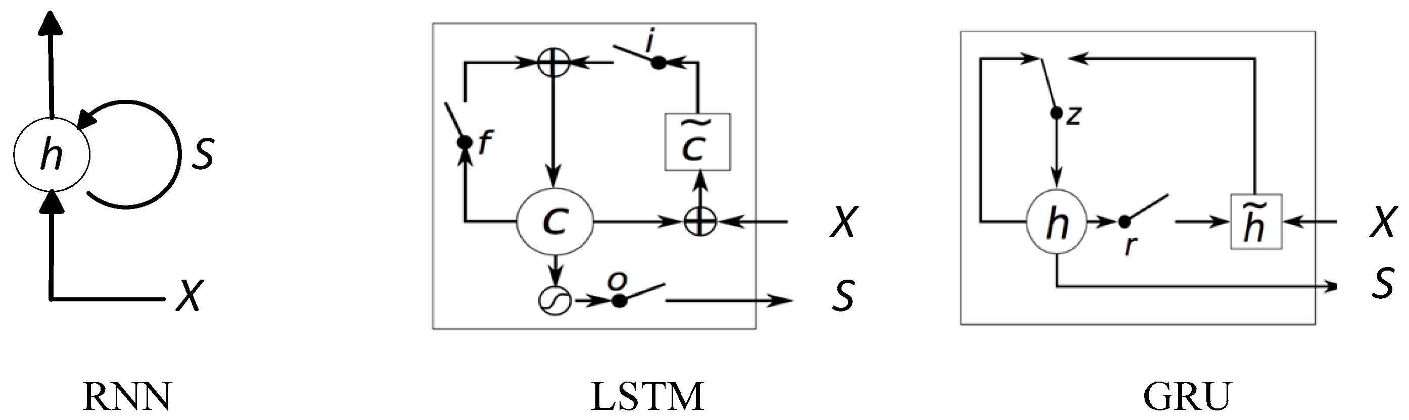
Figure 2.
The structure of Res-RNN and gRes-RNN.

Figure 3.
Best F1 values for the RNN [9], LSTM [16] and GRU [17] and Res-RNN, Res-RNN with gates over epochs.

Figure 4.
Losses for IMDB database of the RNN [9], LSTM [16] and GRU [17] and Res-RNN, Res-RNN with gates over epochs.

Figure 5.
The losses for polyphonic databases of the RNN [9], LSTM [16] and GRU [17] and Res-RNN, Res-RNN with gates in 10,000 epochs.

Figure 6.
Sample of polyphonic music generation by the (a) RNN [9], (b) LSTM [16] and (c) GRU [17], (d) Res-RNN and (e) Res-RNN with gates trained with the databases of Nottingham.

Figure 7.
Sample of polyphonic music generation by the (a) RNN [9], (b) LSTM [16] and (c) GRU [17], (d) Res-RNN and (e) Res-RNN with gates trained with the databases of JSB Chorales.

Figure 8.
Sample of polyphonic music generation by the (a) RNN [9], (b) LSTM [16] and (c) GRU [17], (d) Res-RNN and (e) Res-RNN with gates trained with the databases of Muse Data.
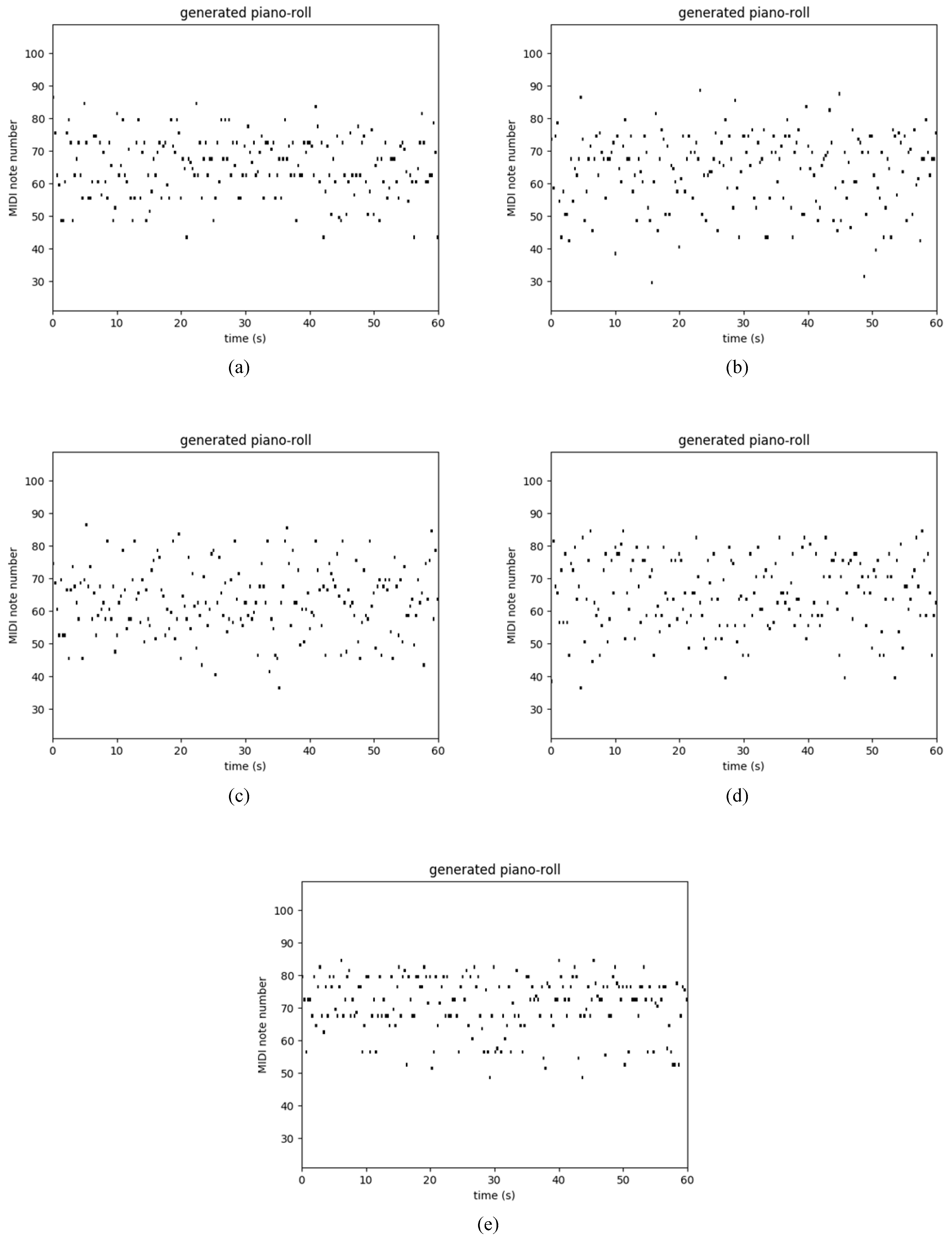
Figure 9.
Sample of polyphonic music generation by the (a) RNN [9], (b) LSTM [16] and (c) GRU [17], (d) Res-RNN and (e) Res-RNN with gates trained with the databases of Piano-midi.


Table 1.
Average performance of the RNN [9], LSTM [16] and GRU [17], Res-RNN and Res-RNN with gates on airline travel information system (ATIS) database [22] in 100 epochs.
| RNN | LSTM | GRU | Res-RNN | gRes-RNN | ||
|---|---|---|---|---|---|---|
| Valid F1 | Mean | 95.63% | 96.58% | 95.63% | 95.87% | 96.53% |
| Std | 0.0142 | 0.0096 | 0.0132 | 0.0115 | 0.0101 | |
| Test F1 | Mean | 92.11% | 93.19% | 92.81% | 92.97% | 93.03% |
| Std | 0.0166 | 0.0092 | 0.0141 | 0.0120 | 0.0110 | |
| Valid Accuracy | Mean | 95.56% | 96.49% | 95.50% | 95.55% | 96.62% |
| Std | 0.0178 | 0.0082 | 0.0122 | 0.0097 | 0.0092 | |
| Test Accuracy | Mean | 91.81% | 92.77% | 92.54% | 92.50% | 92.62% |
| Std | 0.0168 | 0.0077 | 0.0134 | 0.0100 | 0.0083 | |
| Valid Recall | Mean | 95.85% | 96.75% | 96.00% | 96.20% | 96.60% |
| Std | 0.0173 | 0.0056 | 0.0144 | 0.0100 | 0.0099 | |
| Test Recall | Mean | 92.74% | 93.62% | 93.20% | 93.45% | 93.45% |
| Std | 0.0188 | 0.0043 | 0.0112 | 0.0105 | 0.0091 | |
| Time Consumption | 24.10 s | 63.59 s | 56.74 s | 29.10 s | 38.80 s | |
Table 2.
Performance of the RNN [9], LSTM [16] and GRU [17], Res-RNN and Res-RNN with gates on the Internet movie database (IMDB) in 20 epochs.
| Training Accuracy | Test Accuracy | Time Consumption | |||
|---|---|---|---|---|---|
| Mean | Std | Mean | Std | ||
| RNN | 93.91% | 0.0148 | 78.24% | 0.0232 | 51.32 s |
| LSTM | 99.97% | 0.0001 | 85.16% | 0.0023 | 208.44 s |
| GRU | 99.98% | 0.0001 | 85.84% | 0.0038 | 140.10 s |
| Res-RNN | 99.93% | 0.0003 | 84.78% | 0.0042 | 90.08 s |
| Res-RNN with gate | 99.95% | 0.0002 | 85.33% | 0.0029 | 123.22 s |
Table 3.
Average performance of the RNN [9], LSTM [16] and GRU [17] and Res-RNN and Res-RNN with gates on different polyphonic databases in 10,000 epochs.
| RNN | LSTM | GRU | Res-RNN | gRes-RNN | ||
|---|---|---|---|---|---|---|
| Nottingham | Loss | 9.62 | 7.37 | 8.50 | 8.26 | 8.60 |
| Std | 1.63 | 0.54 | 0.72 | 0.89 | 0.66 | |
| Time | 10.45 s | 35.48 s | 27.32 s | 19.06 s | 25.01 s | |
| JSB Chorales | Loss | 9.04 | 7.43 | 8.54 | 7.60 | 7.77 |
| Std | 1.01 | 0.67 | 0.96 | 0.55 | 0.23 | |
| Time | 10.62 s | 35.50 s | 27.14 s | 18.92 s | 25.42 s | |
| MuseData | Loss | 10.42 | 9.62 | 9.86 | 9.31 | 8.93 |
| Std | 1.45 | 0.73 | 0.12 | 0.33 | 0.30 | |
| Time | 10.33 s | 35.39 s | 27.33 s | 19.13 s | 25.01 s | |
| Piano-midi | Loss | 11.71 | 9.57 | 9.62 | 8.22 | 9.26 |
| Std | 1.92 | 0.84 | 0.86 | 0.24 | 0.68 | |
| Time | 10.52 s | 35.44 s | 27.20 s | 19.44 s | 25.01 s | |
© 2018 by the authors. Licensee MDPI, Basel, Switzerland. This article is an open access article distributed under the terms and conditions of the Creative Commons Attribution (CC BY) license (http://creativecommons.org/licenses/by/4.0/).
Share and Cite
MDPI and ACS Style
Yue, B.; Fu, J.; Liang, J. Residual Recurrent Neural Networks for Learning Sequential Representations. Information 2018, 9, 56. https://doi.org/10.3390/info9030056
AMA Style
Yue B, Fu J, Liang J. Residual Recurrent Neural Networks for Learning Sequential Representations. Information. 2018; 9(3):56. https://doi.org/10.3390/info9030056
Chicago/Turabian StyleYue, Boxuan, Junwei Fu, and Jun Liang. 2018. "Residual Recurrent Neural Networks for Learning Sequential Representations" Information 9, no. 3: 56. https://doi.org/10.3390/info9030056
Note that from the first issue of 2016, this journal uses article numbers instead of page numbers. See further details here.