Distributed State Estimation under State Inequality Constraints with Random Communication over Multi-Agent Networks

1
Xi’an Institute of High-Tech, Xi’an 710025, China
2
Institute of Electronics, Chinese Academy of Sciences, Beijing 100190, China
*
Author to whom correspondence should be addressed.
Information 2018, 9(3), 64; https://doi.org/10.3390/info9030064
Submission received: 1 February 2018
/
Revised: 28 February 2018
/
Accepted: 7 March 2018
/
Published: 13 March 2018
Abstract
:In this paper, we investigate distributed state estimation for multi-agent networks with random communication, where the state is constrained by an inequality. In order to deal with the problem of environmental/communication uncertainties and to save energy, we introduce two random schemes, including a random sleep scheme and an event-triggered scheme. With the help of Kalman-consensus filter and projection on the constrained set, we propose two random distributed estimation algorithm. The estimation of each agent is achieved by projecting the consensus estimate, which is obtained by virtue of random exchange information with its neighbors. The estimation error is shown to be bounded with probability one when the agents randomly take the measurement or communicate with their neighbors. We show the stability of proposed algorithm based on Lyapunov method and projection and demonstrate their effectiveness via numerical simulations.
1. Introduction
Recently, state estimation using a multi-agent network have been a hot topic due to its broad range of applications in engineering systems such as robotic networks, area surveillance and smart grids. Distributed method has benefits of robustness and scalability. As one of the popular estimation method, distributed Kalman filter has ability of real-time estimation and non-stationary process tracking.
Distributed Kalman-filter-based (DKF) estimations have been wildly studied in the literatures [1,2,3,4,5,6,7,8,9,10,11]. The idea of references [1,2,5,6,9] is adding consensus term into a traditional Kalman filter structure. For example, in [1], the authors proposed a distributed Kalman filter, where the consensus information state and associated information matrix were used to approximate the global solution. An optimal consensus-based Kalman filter was reported in [2], where all-to-all communication is needed. In order to obtain a practical algorithm, in [2], the authors also reported a scalable distributed Kalman filter, where only the state estimation need to be transmitted between neighbors. Moreover, the switching communication topology for distributed estimation problem was studied in [7,8]. Another kind of distributed Kalman filter design is use the idea of fusing the local estimate of each agent [3,4,10,11]. In [3], the authors investigated distributed Kalman filter by fusing information state of neighbors, and a covariance intersection based distributed Kalman filter was proposed in [4] proposed a diffusion Kalman filter based on covariance intersection method. The last kind of DKF is Consensus+Innovations approach [12,13], which allows each agent tracking the global measurement. It should be notice that the approaches in [12,13] can approximate global optimal solution, which achieved by knowing global pseudo-observations matrix in advance.
New estimation problems emerge resulting from unreliable communication channel and random data packet dropout. In a multi-agent network, KCF was characterized under the effect of lossy sensor networks in [5] by incorporating a Bernoulli random variable in the consensus term. Independent Bernoulli distribution was also used to model the random presence of nonlinear dynamics as well as the quantization effect in the sensor communications in [14]. From an energy saving viewpoint, the agent can be enabled to reduce communication rate. The random sleep scheme (RS) was introduced into the projecting consensus algorithm in [15,16], which allows each agent to choose whether to fall asleep or take action. Different from the RS scheme, there is another well-known scheme, called event-triggered scheme, under which information is transmitted only when the predefined event conditions are satisfied. Assuming the Gaussian properties of the priori conditioned distribution, a deterministic event-triggered schedule was proposed in [17], and, to overcome the limitation of the Gaussian assumption, a stochastic event-triggered scheme was developed and the corresponding exact MMSE estimator was obtained in [18].
On the other hand, in practice, we may obtain some information or knowledge about the state variables, which could be used to improve the performance (such as accuracy or convergence rate) in the design of distributed estimators. In some cases, such knowledge can be described as given constraints of the state variables, which may be obtained from physical laws, geometric relationship, environment constraints, etc. There have been many method to solve the problem of constrained state in Kalman filter, such as pseudo-observations [19], projection [20,21], and moving horizon method [22]. In fact, a survey about the conventional design of Kalman filter with state constraints was reported in [23], and moreover, it showed that the constraints as additional information are useful to improve the estimation performance. In [11], the authors studied distributed estimation with constraints information, where both the state estimation and covariance information are transmitted. In this paper, we concentrate on the problem of distributed estimation under state constraints with random communication, and we use projection method to deal with the constrained state.
In this paper, we focus on distributed estimation under state inequality constraints with random communication, which is an important problem. We design a distributed Kalman filter incorporating consensus term and projection method. Specifically, the constrained estimate obtained in each agent by projecting the consensus estimation onto the constrained surface. Moreover, in order to reduce the communication efficiently, we introduce a stochastic event triggered scheme to realize a tradeoff between communication rate and performance. We summarize the contribution of the paper as follows: (i) We proposed a distributed Kalman filer with state inequity constraints and stochastic communication. (ii) We introduce random sleep scheme and stochastic event-triggered scheme to reduce the communication rate. (iii) We analyze the stability properties of proposed algorithm by Lyapunov method.
The remainder of the paper is organized as follows. Section 2 provide some necessary preliminaries and formulate the distributed estimation problem with state constriants and random communication. Section 3 give algorithms based on random sleep scheme and stochastic event-triggered scheme. The performance analysis are provided in Section 4, and then a numerical simulation is shown in Section 5, which shows the benefit of state constraints. Section 6 give the discussions of the paper. Finally, some concluding remarks are provided in Section 7.
Notations: The set of real number is denoted by . A symmetric matrix is denoted by M, and a positive definite matrix is () means that the matrix is positive semi-definite (definite). The maximum and minimum eigenvalue are denoted by and , respectively. represents mathematical expectation. denotes the probability of random variable .
2. Problem Formulation
In this section, we first provide some preliminaries about convex analysis [24]. Then the problem of distributed estimation with state constraints and random communication is formulated.
2.1. Preliminaries
Consider a function , if for any and , holds, then is a convex function. Similarly, if for any and , holds, then is a convex set. Denote is the projection onto a closed and convex subset X, which has following definition:
In order to analyze the properties of proposed algorithm, we provide a lemma about projection (see [25]).
Lemma 1.
Let X be a closed convex set in . Then
- (i)
- , for all ;
- (ii)
- , for all x and z;
- (iii)
- , for any .
2.2. Problem Formulation
Consider the following linear dynamics
where is the states, is zero-mean and covariance Gaussian white noises.
In practice, according to the physical laws or design specification, some additional information is known as prior knowledge, which can be formulated as inequality constriants about state variables (some engineering applications can be found in [23]). In this paper, we consider the state inequality constraints [26,27,28]. Specifically, for the dynamics (1), the inequality constraints about the state can be given as follows,
where is a convex function, s is the number of the constraints.
State is estimated by a network consisting of N agents. The measurement equation of the ith agent is given by:
where , is the measurement noises by agent i which is assumed to be zero-mean white Gaussian with covariance . is independent of and is independent of when or .
Graph theory [29] can be used to describe the communication topology of the network, where the agent i can be treated as node i, and the edge can be regarded as communication link. An undirected graph is denoted as , where is the node set, and is the edge set. If node i and node j are connected by an edge, then these two vertices are called adjacent. The neighbor set of node i is defined by . Denote as the weighted adjacency matrix of , where the element and , and the corresponding Laplacian is L. The weighted adjacency matrix of graph is defined as , where and . Denote the Laplacian of the weighted graph is L. It is well known that, for Laplacian L associated with graph , if is connected, then and .
In this paper, we adopt the following two standard assumptions, which have been widely used.
Assumption 1.
is detectable and is controllable.
Assumption 2.
The undirected graph is connected.
The Kalman-consensus filter is designed by using local measurement and information from neighbors, which was given in [2],
where is the estimate by each agent. is the consensus gain, and are the estimator gain and consensus gain need to be designed, respectively.
In order to satisfy the state constraints (2), the estimate obtained by each agent should solve the following optimization problem:
where . In this paper, we assume that each agent knows the constraints (2), and therefore, the constrained estimation can be obtained by projection at each agent. Namely,
with . The aim of distributed estimator (4) is to find the optimal gain and to minimize the mean-squared estimation error .
Different with existing works in [2,7,8], which did not consider any state constraints and random communication. Here, we consider the problem of constrained KCF with random communication. Moreover, due to the uncertainty environment and saving energy, agents may loss measurement or random communication with neighbors. Hence, to solve our problem, we need to show how to design the Kalman filter gain and the consensus gain under random communication such that the estimation error of (6) is bounded.
In the following section, we introduce random sleep and event-triggered scheme to design distributed estimation algorithm, and then analyze the stability conditions of the proposed algorithms.
3. Distributed Algorithms
We present two algorithms in the following subsections, respectively.
3.1. Random Sleep Algorithm
In practice, the communication cost may be much larger than the computational cost. Hence it is reasonable to reduce the communication rate and to save energy. Here we introduce a random sleep (RS) scheme, which allows the agents to have their own policies to collect measurement or send message to its neighbors. To be specific, in our RS scheme, the agents may fall in sleep during the measurement collection and consensus stage with independent Bernoulli decision, respectively. When a agent sleeps during the measurement collection, it cannot use measurement to update the local estimate. When it sleeps during the consensus stage, it cannot send any information to its neighbors.
Let and be given constants. Denote and as independent Bernoulli random variables with , , and , . We make the following assumptions,
Furthermore, notice that , , and , .
Then we propose a distributed random sleep algorithm for the Kalman-filter-based estimation as follows:
If we ignore consensus step, the covariance iteration and the gain can be obtained by the minimum mean squared error (MMSE) estimation as follows (see [30]):
To ensure that the estimate by each agent always satisfies the constraints, we present the following algorithm by projecting the unconstrained estimation onto the constrained surfaces:
The proposed Kalman-consensus filter with constraints via RS scheme (RSKCF) is summarized in Algorithm 2.
Define and . According to Lemma 1, , which hints that the estimator can achieve better performance using the constraint information in the design. In [20], the author proved that the projection-based Kalman filter with linear equality constraints performs better than unconstrained estimation.
Notice that in the algorithm does not represent the estimation error covariance with respect to any longer. A poor choice of consensus gain may spoil the stability of the error dynamics. In section IV, we will present the stability analysis of the algorithm with an appropriate choice of the consensus gain.
| Algorithm 1 KCF with constraints via RS (RSKCF) |
At time k, a prior information Initialization , ; Random Sleep on Measurement Collection Random Sleep on Consensus Projection |
Define , then the error dynamics of Algorithm 1 can be written as
Remark 1.
The different choices of and correspond to different network conditions. If and , the network is not connected, and each agent only computes the estimate by its local Kalman filter with constraints. If and , the multi-agent system has a perfect communication channel but each agent may fall in sleep during the measurement collection. When and , each agent produces measurement at each time but maybe fall in sleep during the consensus stage. Since the RS probability and can be determined independently, we can take the advantage of the formulation to simplify the design in practice.
Remark 2.
It should be notice that the inequality constraints in this paper including the linear equality constraints. In section IV, the problem (4) will be solved in closed-form under linear equality constraints as a special case, which consistent with the case in [20]. It also should be notice that, the nonlinear equality constraints cannot be solve by projection method, because may not be a convex set.
3.2. Stochastic Event-Triggered Scheme
An event-triggered scheme, based on an event monitor, can also be considered to reduce the communication rate and to save energy. The event-triggered idea is carried out as follows: when the associated monitor exceeds a predefined threshold, the agent transmits local information with its neighbors, which provides a tradeoff between the communication rate and the performance. Since the agents only transmit valuable information, the event-triggered scheme may achieve better performance compared with the proposed RS scheme. In [17,18], the authors dealt with a centralized stochastic event-triggered estimation problem. Here we introduce a distributed stochastic event-triggered scheme by extending the algorithms described in [18].
Denote a binary decision variable for agent i at time k. We use the following strategy: agent i measures the target state and sends information to its neighbors if ; agent i only receives information from its neighbors if . As stated in [18], at each time instant, agent i generates an i.i.d random variable and computes as follows:
where , and . Clearly, in (13), the parameter introduces one degree of freedom to balance the tradeoff between the communication rate and the estimation performance. From an engineering viewpoint, a larger means more information to be transmitted.
The local MMSE estimator (without consensus and projection) for agent i with incorporating the stochastic event-triggering (13) is given as follows (see Theorem 2 in [18]):
As stated before, by the consensus idea and projection technique, the constrained estimation can be obtained by . The stochastic event-triggered KCF with constraints (ETKCF) is described in Algorithm 2.
| Algorithm 2 KCF with constraints via stochastic event-triggered scheme |
Initialization ; Local Estimation Consensus Projection |
Remark 3.
Since only the important information is broadcasted, the stochastic event-triggered scheme may achieve better performance compared with the RS scheme. The RS scheme, however, has a simpler form and is easier to implement.
Remark 4.
Here, we provide some notations, which will help to analysis the proposed algorithms. For given A, , Q, and , without loss of generality, there are positive scalars , , , , , and such that
4. Performance Analysis
In this section, we analyze the convergence of the proposed algorithms in the following three subsections. We introduce some concepts related to stochastic processes, which are useful in the following convergence analysis ([31,32]).
Definition 1.
The stochastic process is said to be exponential bounded in mean square, if there are real numbers, , and such that
holds for every .
Definition 2.
The stochastic process is said to be bounded with probability one, if
holds with probability one.
We first give three lemmas, which can be found in [33].
Lemma 2
(Lemma 2.1, [33]). Suppose that there is a stochastic process as well as positive numbers , , μ, and such that
and
are fulfilled. Then the stochastic process is exponentially bounded in mean square, i.e.,
for every . Moreover, the stochastic process is bounded with probability one.
Lemma 3
Lemma 4
4.1. Random Sleep Scheme
The following theorem shows the stochastic stability of (12).
Theorem 1.
Under Assumptions 1 and 2, the error dynamics (12) for Algorithm 1 is exponentially bounded in mean square and bounded with probability one.
To prove the Theorem 1, we give a lemma first. Its proof can be found in Appendix A.
Lemma 5.
Under Assumptions 1, there exists a constant such that
holds.
Proof of Theorem 1.
By Lemma 4, there exists a constant such that
The error dynamics of Algorithm 1 is
With , we have
where . By (24) and Lemma 5, and taking expectation on both side of above equation, we have
where .
Similarly, the consensus gain can be choosen as , where . Denoting , we have
where and defined as
According to Lemma 5, , where . Substituting it into (29) yields
Take with
Obviously, Lemma 2 can be satisfied with
Thus, the conclusion follows. ☐
Remark 5.
From the proofs of Theorems 1, the constrained estimation is the same as unconstrained estimation once for agent i. Otherwise, . In other words, the constrained estimation is closer to the true state than the unconstrained estimation . In fact, our schemes first make all agents’ estimation error bounded, and then project each estimation onto the surface of constraints.
Remark 6.
It should be notice that, if the system is asymptotically stable, i.e., the spectral radius of A is less than 1, there alway exists the gains to guarantee the convergence of MSE. When the system is unstable, i.e., the spectral radius of A greater than 1, we need to design estimation gain and to guarantee the convergence of MSE. In [13], the authors discussed the maximum degree of instability of A, that guarantees the convergence of distributed estimation algorithm. The maximum degree of instability of A relates with connectivity and global measurement matrix, which reflects the tracking ability of the networks. Given the maximum degree of A, the problem remains how to design the gain matrices and .
In what follows, we give the closed-form solution under linear equality constraints, which can be written as follows:
where is constraint matrix, , and s is the number of constraints. Generally, D should be of full rank, otherwise, we have redundant constraints. In such case, we can remove linearly dependent rows from D until D is of full rank.
In order to use projection method, the constraints (32) can be written as . For each individual agent, we can obtain the constrained estimate by projection as follows:
where is the estimate obtained by the consensus step. Therefore, we have the following result.
Corollary 1.
Under Assumptions 1 and 2, the error dynamics of the Algorithm 1 with constraints (32) is exponentially bounded in mean square and bounded with probability one. Moreover, the constrained estimation is .
Clearly, linear equality constraints can be extended to the linear state inequality constraints . Specifically, if the consensus estimate step satisfies , then constrained estimation and will be the same. Otherwise, the constrained estimate can be obtained by projecting onto . Therefore, the Corollary 1 still holds for the linear inequality constraints case.
4.2. Event-Triggered Scheme
The communication rate for agent i can be achieved by
Notice that is proportional to the probability density of Gaussian variable. If we can obtain the covariance of in the steady state, we can obtain the communication rate [18]. However, it is difficult to analyze the communication rate since depends on the consensus and projection stage in the distributed case, though a communication rate is determined using the stochastic event-triggered scheme (13).
Although we cannot explicitly obtain the stochastic event-triggered communication rate, we can still easily find that the event-triggered scheme performs better than the random sleep scheme having the same communication cost (referring to the the performance comparison between random sleep scheme and stochastic event-triggered scheme by simulations as shown in Section 5).
Actually, for agent i, there exists a stochastic event-triggered communication rate . The probability of collection measurements and sending information can be taken as 1 and , respectively. Following Theorem 1, there exists a sufficient small consensus gain to guarantee that the error dynamics is exponentially bounded in mean square and bounded with probability one.
5. Simulations
In this section, we give some simulations to illustrate the effectiveness of proposed algorithms. We compare the estimation performances of the proposed estimator with the suboptimal consensus-based Kalman filter (SKCF) in [2]. Moreover, we compare the performance between proposed two algorithms.
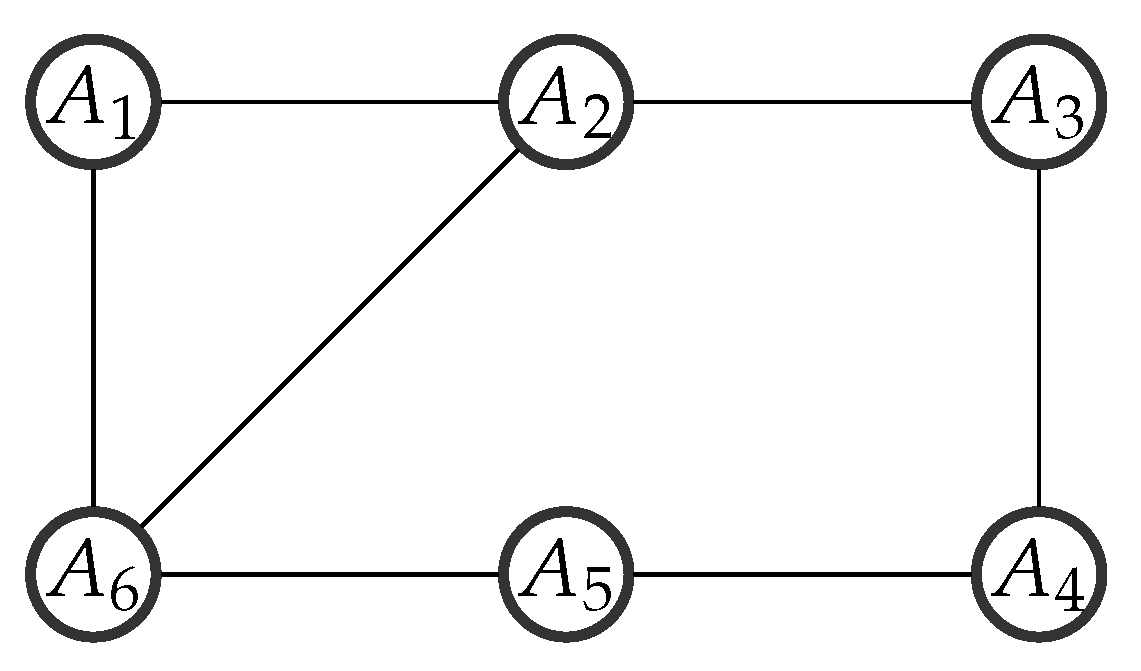
A target moves along a line with constant velocity, which is tracked by a network with agents. The topology of the network is shown in Figure 1. The dynamics of target is given as follows
where T is the sampling period, . and are the target position, and and are the velocity along different directions. In this example, we take and .
The measurement by agent i is expressed as follows,
In [20], the author stated that the target is constrained if it is traveling along the road, otherwise, it is unconstrained. In this example, we assume the target is along a given road, and therefore, the problem is constrained. Here we consider that the target is travelling on a road with a heading of , which means . Then the constrained information can be written as:
In this example, we take .
Simulation Case 1: In this case, we test the performance of proposed two algorithms. Denote , , and initial conditions by agent i is set to , ,, , , , .
We consider the total mean square estimation errors (TMSEE) of Algorithm 1, and compare its performance with the existing consensus-based Kalman filter algorithms in [9]. Here, we name the algorithm in [9] as SKCF. TMSEE is widely used to indicate the performance of the estimator, which is defined as
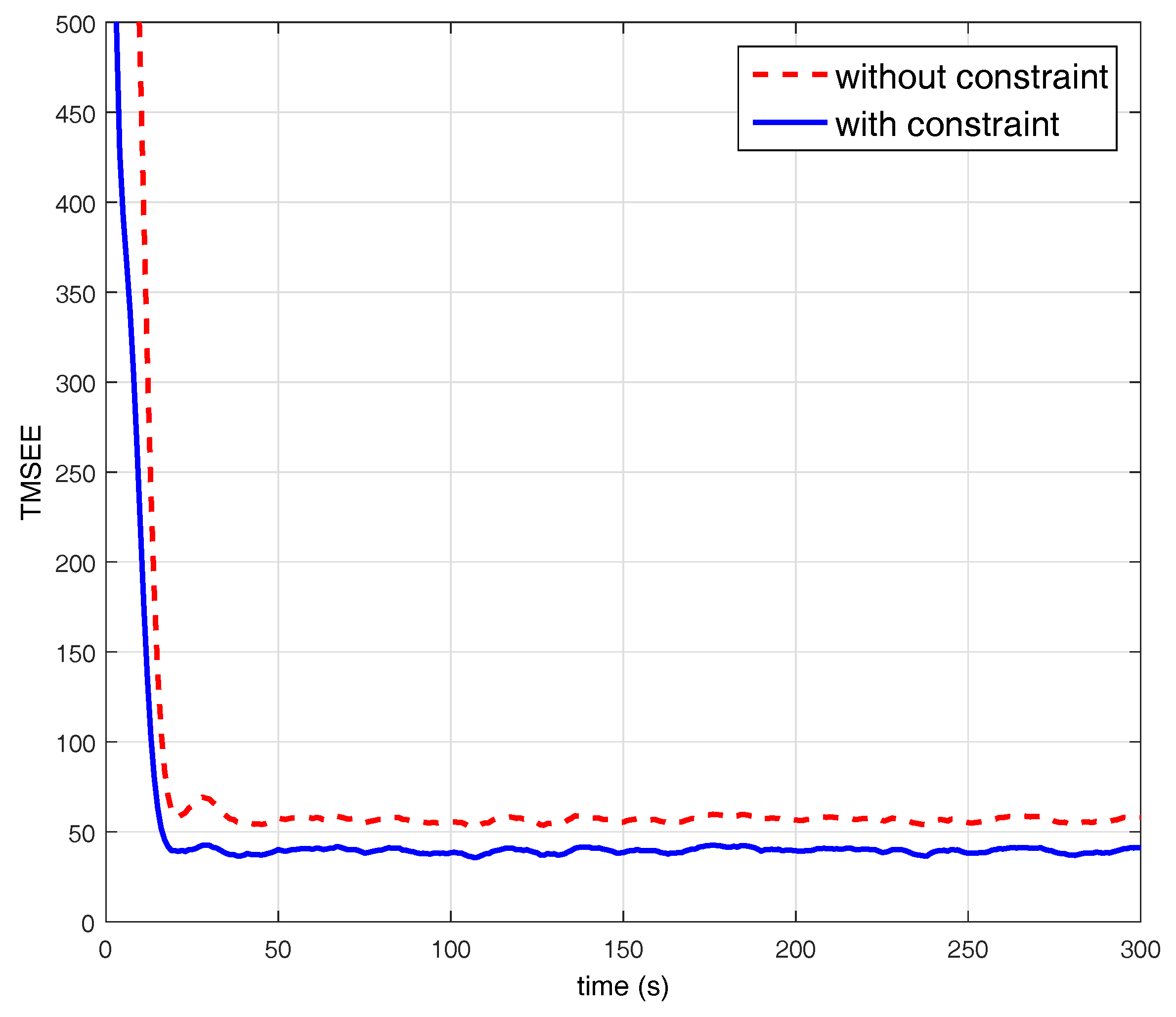
The parameters of the multi-agent system are chosen that the upper bound on g is determined by Theorem 1. In both cases, 1000 times independent Monte Carlo simulations are carried out to show the estimation performance. Figure 2 shows the TMSEE of Algorithm 1 and SKCF in [9] with the same communication rate. It can be seen that the constrained estimation by Algorithm 1 is more accurate than the unconstrained KCF. Moreover, according to Figure 2, it is clear that the RSKCF with the constraints converges to a precision of 60 in less than 15 instances while SKCF without any constraints needs almost 20 instances. Therefore, for this example based on the constraint information, the proposed RSKCF with the constraints outperforms SKCF in both convergence rate and accuracy.
Next, we give the simulation results of Algorithm 1. The parameters setting is the same as above. Take , and . Figure 3 shows that the estimation error of the agents can reach consensus and bounded, which is consistent with the results of Theorem 1.
The curve of with fixed is shown in Figure 4, while the curve with fixed is shown in Figure 5. From the proof of Theorem 1 it can be observed that the upper bound for g increases along with the probability of collection measurements. Moreover, the upper bound for g decreases along with the probability of broadcast accordingly.
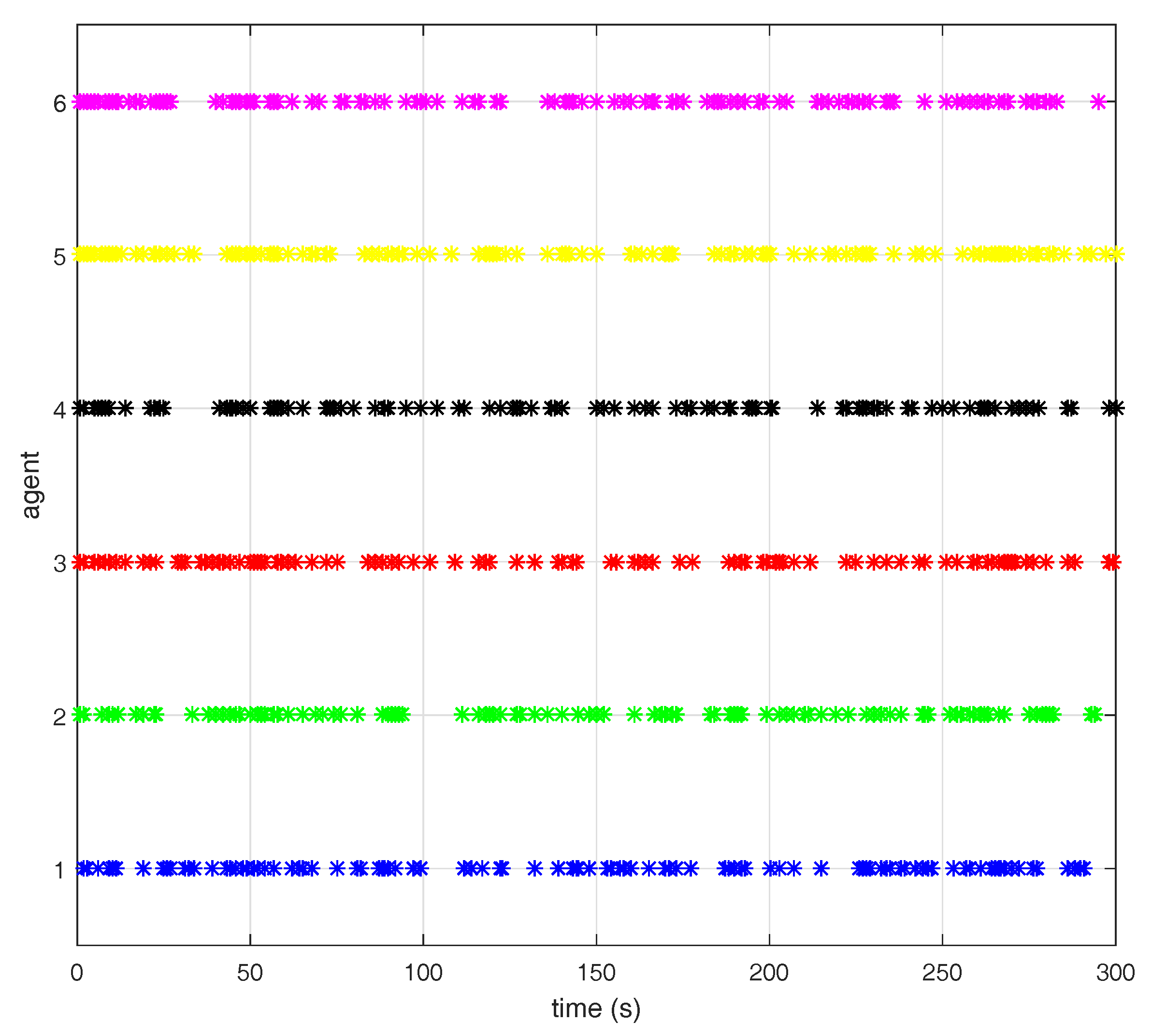
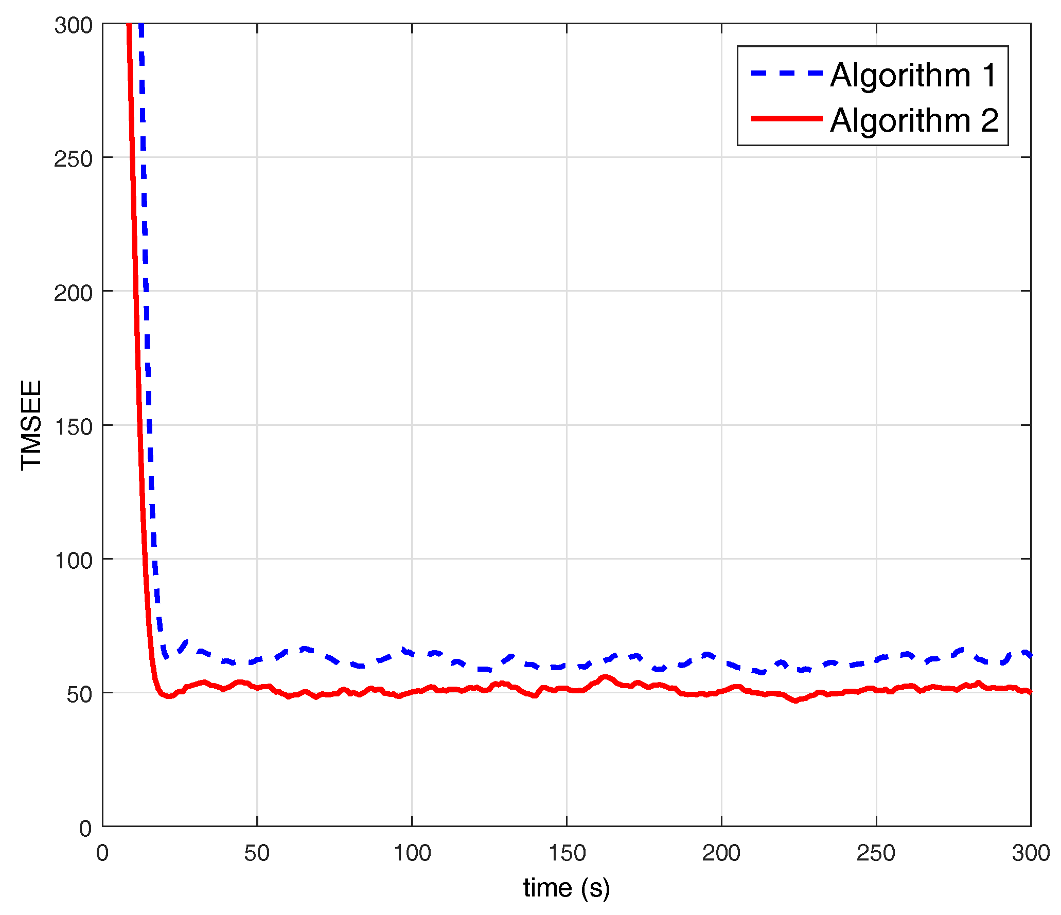
In order to compare the performance between stochastic event-triggered scheme and random sleep scheme, we choose parameters to ensure that and . Specifically, we can obtain that , , , , and by simulations. The triggering sequence are shown in Figure 6. The stochastic event-triggered scheme performs better than the random sleep scheme as shown in Figure 7. An intuitive explanation is that, only important information is transmitted by stochastic event-triggered scheme. The communication rate of Algorithm 2 with , , , , are shown in Figure 8, where . The simulation results show that the communication rate increases along with the increasing of , since the agent will be more likely to share the information with its neighbors along with the increasing of based on the event-triggered scheme (13).
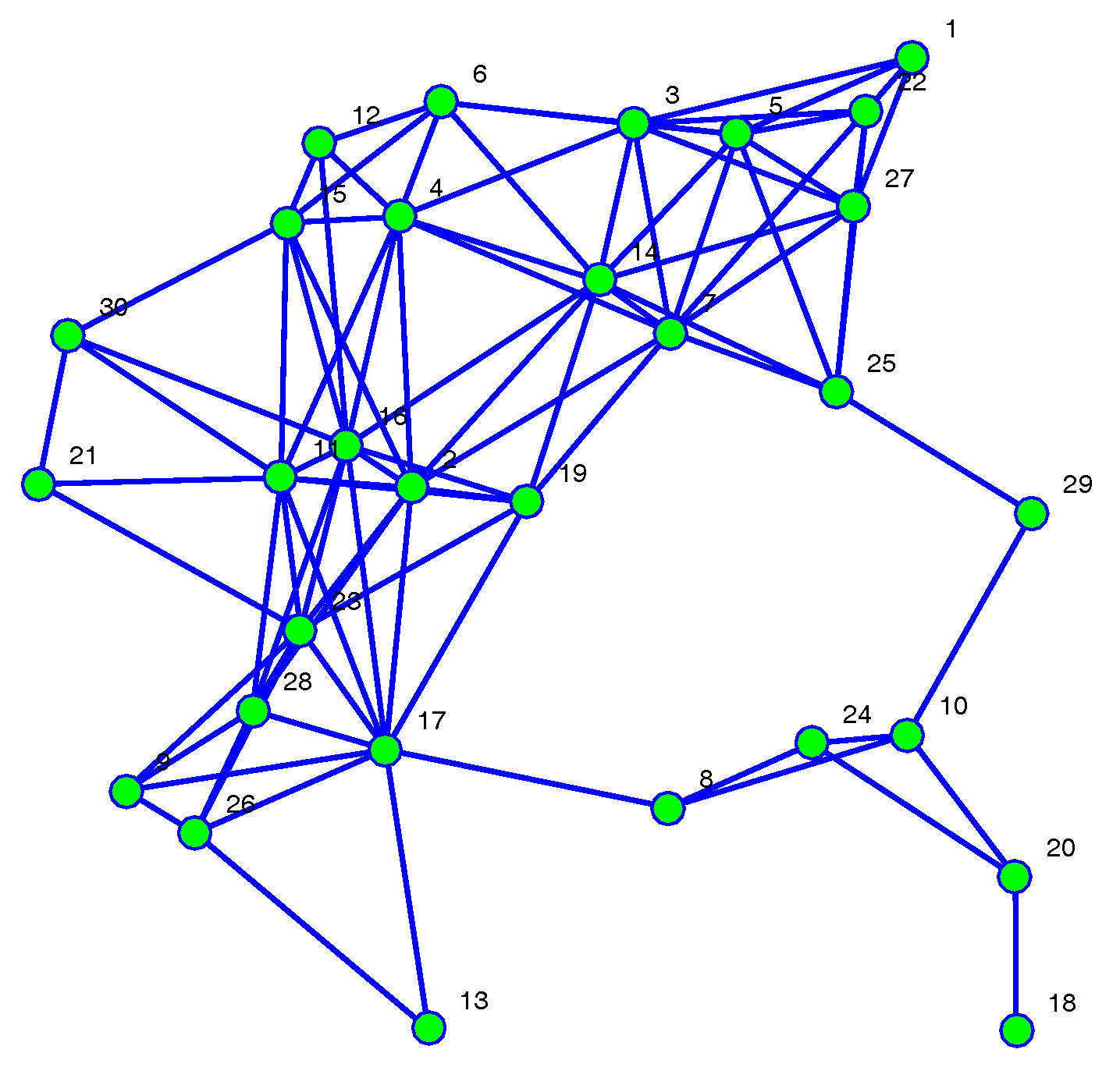
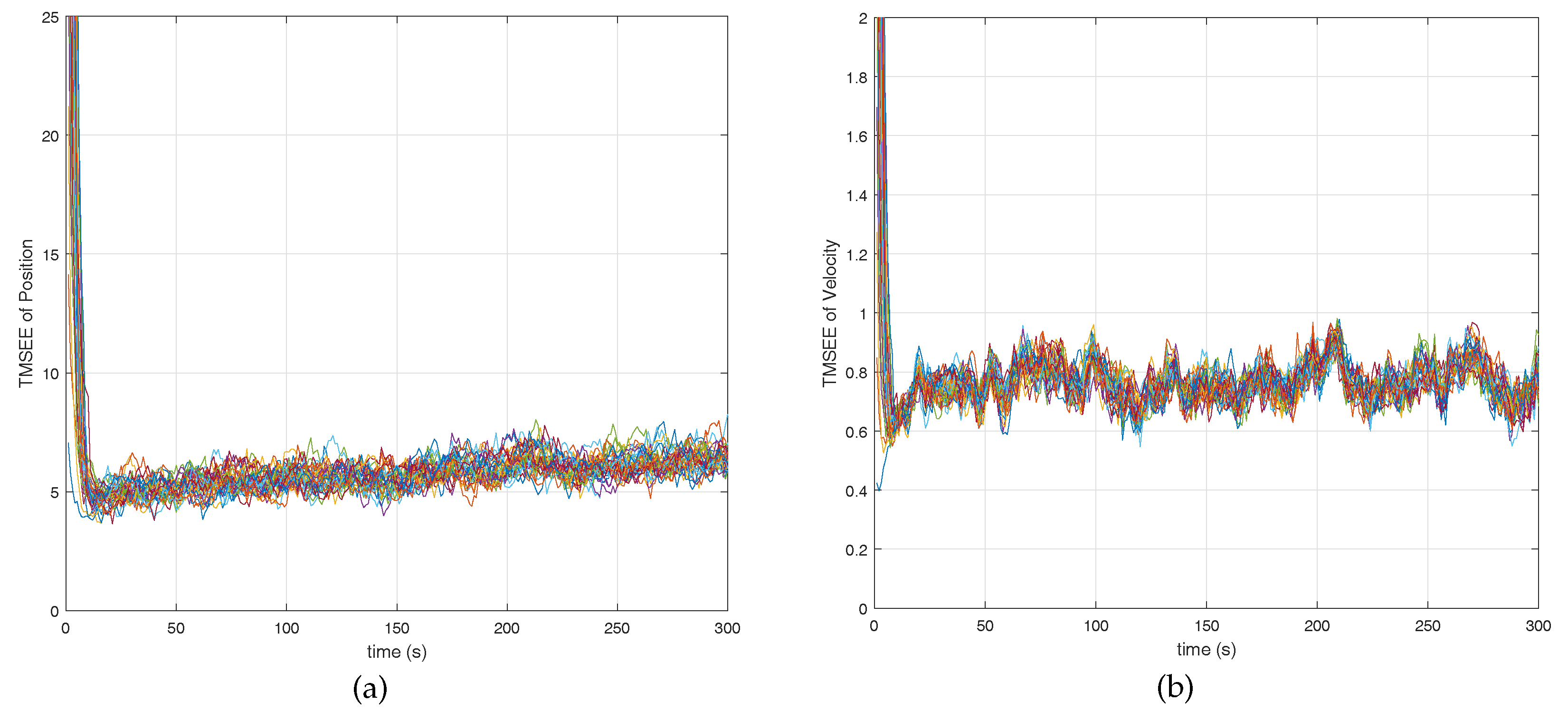
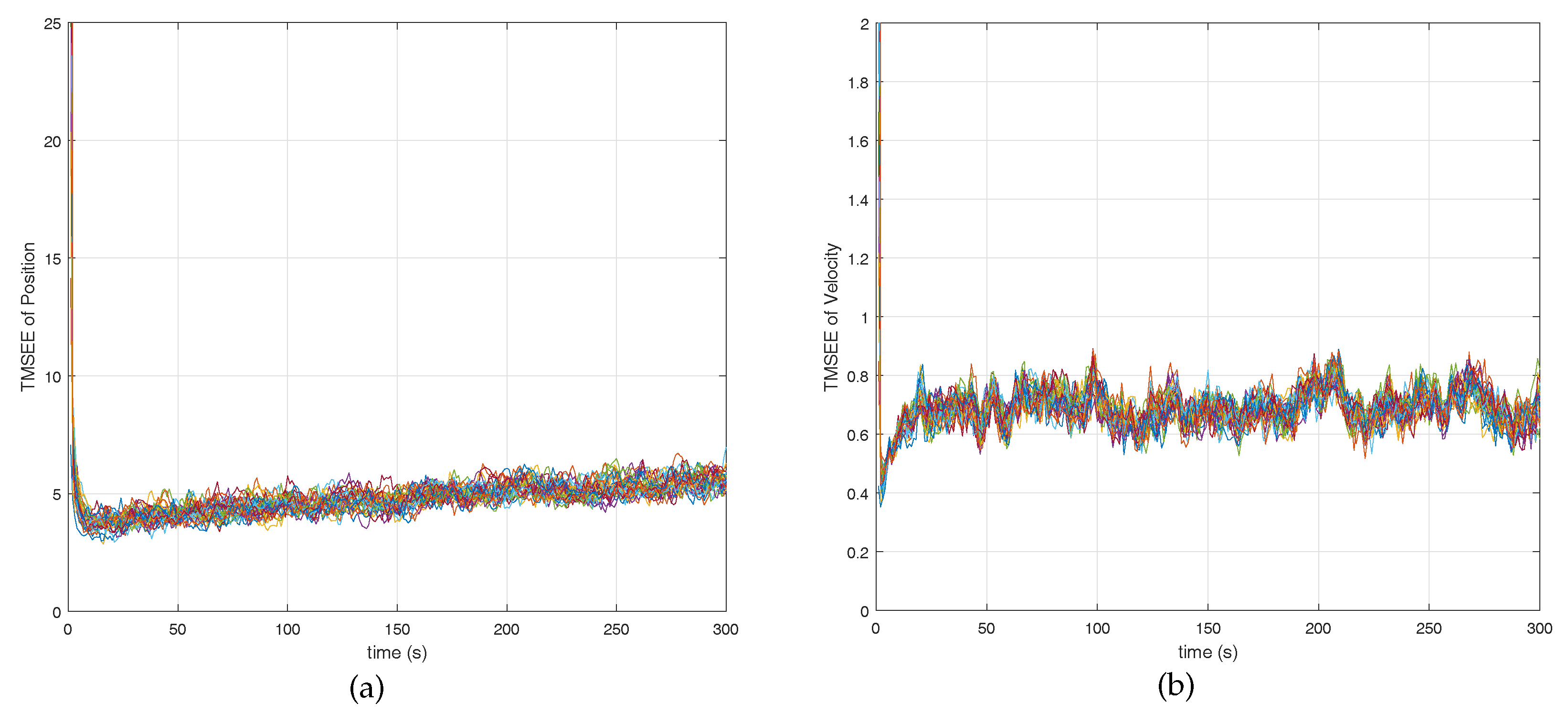
Simulation Case 2: In this case, we give an example in a complex network, i.e., the network consists of 30 agents. The communication topology of the network shown in Figure 9. The parameters setting is the same as case 1. The initial conditions by agent i is set to , , where and are taking from randomly. Figure 10 shows the comparison between Algorithms 1 and 2. From Figure 10, we can see that the stochastic event-triggered scheme still performs better than random sleep scheme Figure 11 and Figure 12 give the TMSEE of Algorithms 1 and 2, respectively.
6. Discussion
As shown in Figure 2, the proposed algorithm can achieve better performance comparing with the one in [9]. It is due to that the constraints information can be treated as additional information, and such additional information beyond those explicitly given in system model. Therefore, the description of modified model is different with the standard Kalman filter equations, and the modified one can help to improve the estimation performance. In [34], the authors studied estimation with nonlinear equality constraints, where the nonlinear state constraints are linearization locally and the estimation was obtained by projection to local linear surface. When it comes to distributed setting, such linearization will produce approximation error and may suffer from a lack of convergence. Our future study may include designing distributed filtering with nonlinear state equality constraints.
A consensus-based Kalman filter with stochastic sensor activation was proposed in [5], where all sensors share the same activation probability, and the stability of the algorithm was proved. In [9], the authors extended the results to different activation probability of each sensor, and the convergence property was shown under mild condition. Both [5] and [9] studied mean-square stability of the algorithm. Differently, we study the stochastic stability of the proposed algorithm, and show that the constraints information will help to improve the estimation performance.
In this paper, we investigate the random communication problem for distributed estimation with state constraints. It should be notice that local observability condition was needed. In [11], the authors also studied distributed estimation problem with state inequality constraints for deterministic case, where the global observability condition was needed, i.e., each agent need not to be observable. The results in [11] relies on the sufficient communication between agents so that the information will spread to whole network. However, when agent communicates with neighbors randomly, the information will not spread enough to whole network. Therefore, the global observability hard to guarantee the stability of estimation. Under global observability, it can be easy to see that if agents are not communicating with each other, the estimation will diverge. It is worth studying how to design the communication rate such that the estimation error is stable under global observability condition.
In [35,36], the distributed event-triggered estimation was also studied. In [35], a time-varying gain was designed by Riccati-like difference equations in order to adjust the innovative and state-consensus information, while, in [36], an event-triggered scheme was provided by analyzing the stability conditions of the error dynamics (without noise terms). Motivated by [18], we introduce the stochastic event-triggered scheme [18], which shown how to design a parameter in the event mechanism satisfying a desired trade-off between the communication rate and the estimation quality. However, in distributed setting, it is hard to obtain the communication rate due to the correlation between agents. In future we may study the communication rate for distributed stochastic event-triggered estimation.
There exist a lot of works to investigate network structures [37,38,39,40]. In [37], the authors presented a metrics suite for evaluating the communication of the multi-agent systems, where one agent can choose any agent to communicate. The paper [38] considered the problem of network-based practical set consensus over multi-agent systems subject to input saturation constraints with quantization and network-induced delays. We considered distributed estimation problem over multi-agent systems without input, quantization and delays, which can be our future works. In [39], the authors considered the problem of permutation routing over wireless networks. The main idea in [39] is to partition the network into several groups. Then, broadcasting is performed locally in each group and getaways are used for communication between groups to send the items to their final destinations.
7. Conclusions
Distributed estimation based on the Kalman filter under state constraints with random communication was proposed in this paper. Two stochastic schemes, that is, the random sleep and event-triggered schemes, were introduced to deal with the environment or communication uncertainties and for energy saving. The convergence of the proposed algorithms was verified, and the conditions for the corresponding stability were given by choosing a suitable consensus gain. Moreover, it was shown that the information of additional state constraints is useful to improve the performance of distributed estimators.
Acknowledgments
This work was partially supported by national natural science foundations of China 61403399.
Author Contributions
Chen Hu, Haoshen Lin, Zhenhua Li, Bing He and Gang Liu contributed to the idea. Chen Hu developed the algorithm, and Chen Hu, Haoshen Lin collected the data and performed the simulations. Chen Hu, Haoshen Lin and Zhenhua Li analyzed the experimental results and wrote this paper. Bing He and Gang Liu supervised the study and reviewed this paper.
Conflicts of Interest
The authors declare no conflict of interest.
Appendix A. Proof of Lemma 5
Proof of Lemma 5.
Equation (9) can be written as
It can be verified that
By applying the matrix inverse lemma (see [41], Appendix A.22, p. 487), we have
Similarly, we obtain
Moreover, it follows from and that
As a result,
Notice that ,
Taking the inverse of both sides of (A10), multiplying from left and right with and , respectively, and then taking expectation operator on the both sides, we obtain
with
☐
References
- Olfati-Saber, R. Distributed Kalman filtering for sensor networks. In Proceedings of the IEEE Conference on Decision and Control, New Orleans, LA, USA, 12–14 December 2007; pp. 5492–5498. [Google Scholar]
- Olfati-Saber, R. Kalman-consensus filter: Optimality, stability, and performance. In Proceedings of the Joint IEEE Conference on Decision and Control and Chinese Control Conference, Shanghai, China, 15–18 Decmber 2009; pp. 7036–7042. [Google Scholar]
- Cattivelli, F.; Sayed, A. Diffusion strategies for distributed Kalman filtering and smoothing. IEEE Trans. Autom. Control 2010, 55, 2069–2084. [Google Scholar] [CrossRef]
- Hu, J.; Xie, L.; Zhang, C. Diffusion Kalman Filtering Based on Covariance Intersection. IEEE Trans. Signal Process. 2012, 60, 891–902. [Google Scholar] [CrossRef]
- Yang, W.; Chen, G.; Wang, X.; Shi, L. Stochastic sensor activation for distributed state estimation over a sensor network. Automatica 2014, 50, 2070–2076. [Google Scholar] [CrossRef]
- Stanković, S.; Stanković, M.; Stipanović, D. Consensus based overlapping decentralized estimation with missing observations and communication faults. Automatica 2009, 45, 1397–1406. [Google Scholar] [CrossRef]
- Zhou, Z.; Fang, H.; Hong, Y. Distributed estimation for moving target based on state-consensus strategy. IEEE Trans. Autom. Control 2013, 58, 2096–2101. [Google Scholar] [CrossRef]
- Hu, C.; Qin, W.; He, B.; Liu, G. Distributed H∞ estimation for moving target under switching multi-agent network. Kybernetika 2014, 51, 814–819. [Google Scholar]
- Yang, W.; Yang, C.; Shi, H.; Shi, L.; Chen, G. Stochastic link activation for distributed filtering under sensor power constraint. Automatica 2017, 75, 109–118. [Google Scholar] [CrossRef]
- Ji, H.; Lewis, F.L.; Hou, Z.; Mikulski, D. Distributed information-weighted Kalman consensus filter for sensor networks. Automatica 2017, 77, 18–30. [Google Scholar] [CrossRef]
- Hu, C.; Qin, W.; Li, Z.; He, B.; Liu, G. Consensus-based state estimation for multi-agent systems with constraint information. Kybernetika 2017, 53, 545–561. [Google Scholar] [CrossRef]
- Das, S.; Moura, J.M. Distributed Kalman filtering with dynamic observations consensus. IEEE Trans. Signal Process. 2015, 63, 4458–4473. [Google Scholar]
- Das, S.; Moura, J.M. Consensus+ innovations distributed Kalman filter with optimized gains. IEEE Trans. Signal Process. 2017, 65, 467–481. [Google Scholar] [CrossRef]
- Dong, H.; Wang, Z.; Gao, H. Distributed Filtering for a Class of Time-Varying Systems Over Sensor Networks With Quantization Errors and Successive Packet Dropouts. IEEE Trans. Signal Process. 2012, 60, 3164–3173. [Google Scholar] [CrossRef]
- Lou, Y.; Shi, G.; Johansson, K.; Henrik, K.; Hong, Y. Convergence of random sleep algorithms for optimal consensus. Syst. Control Lett. 2013, 62, 1196–1202. [Google Scholar] [CrossRef]
- Yi, P.; Hong, Y. Stochastic sub-gradient algorithm for distributed optimization with random sleep scheme. Control Theory Technol. 2015, 13, 333–347. [Google Scholar] [CrossRef]
- Wu, J.; Jia, Q.; Johansson, K.; Shi, L. Event-based sensor data scheduling: Trade-off between communication rate and estimation quality. IEEE Trans. Autom. Control 2013, 58, 1041–1046. [Google Scholar] [CrossRef]
- Han, D.; Mo, Y.; Wu, J.; Weerakkody, S.; Sinopoli, B.; Shi, L. Stochastic event-triggered sensor schedule for remote state estimation. IEEE Trans. Autom. Control 2015, 60, 2661–2675. [Google Scholar] [CrossRef]
- Julier, S.; LaViola, J. On Kalman filtering with nonlinear equality constraints. IEEE Trans. Signal Process. 2007, 55, 2774–2784. [Google Scholar] [CrossRef]
- Simon, D.; Chia, T.L. Kalman filtering with state equality constraints. IEEE Trans. Aerosp. Electron. Syst. 2002, 38, 128–136. [Google Scholar] [CrossRef]
- Ko, S.; Bitmead, R. State estimation for linear systems with state equality constraints. Automatica 2007, 43, 1363–1368. [Google Scholar] [CrossRef]
- Rao, C.; Rawlings, J.; Lee, J. Constrained linear state estimation—A moving horizon approach. IEEE Trans. Aerosp. Electron. Syst. 2001, 37, 1619–1628. [Google Scholar] [CrossRef]
- Simon, D. Kalman filtering with state constraints: A survey of linear and nonlinear algorithms. IET Control Theory Appl. 2010, 4, 1303–1318. [Google Scholar] [CrossRef]
- Boyd, S.; Vandenberghe, L. Convex Optimization; Cambridge University Press: Cambridge, UK, 2004. [Google Scholar]
- Nedić, A.; Ozdaglar, A.; Parrilo, P. Constrained consensus and optimization in multi-agent networks. IEEE Trans. Autom. Control 2010, 55, 922–938. [Google Scholar] [CrossRef]
- Bell, B.; Burke, J.; Pillonetto, G. An inequality constrained nonlinear Kalman-Bucy smoother by interior point likelihood maximization. Automatica 2009, 45, 25–33. [Google Scholar] [CrossRef]
- Simon, D.; Simon, D. Kalman filtering with inequality constraints for turbofan engine health estimation. IEE Proc. Control Theory Appl. 2006, 153, 371–378. [Google Scholar] [CrossRef]
- Goodwin, G.; Seron, M.; Doná, J.D. Constrained Control and Estimation: An Optimisation Approach; Springer: New York, NY, USA, 2006. [Google Scholar]
- Godsil, C.; Royle, G. Algebraic Graph Theory; Springer: New York, NY, USA, 2001. [Google Scholar]
- Sinopoli, B.; Schenato, L.; Franceschetti, M.; Poolla, K.; Jordan, M.I.; Sastry, S.S. Kalman filtering with intermittent observations. IEEE Trans. Autom. Control 2004, 49, 1453–1464. [Google Scholar] [CrossRef]
- Agniel, R.; Jury, E. Almost sure boundedness of randomly sampled systems. SIAM J. Control 1971, 9, 372–384. [Google Scholar] [CrossRef]
- Tarn, T.; Rasis, Y. Observers for nonlinear stochastic systems. IEEE Trans. Autom. Control 1976, 21, 441–448. [Google Scholar] [CrossRef]
- Reif, K.; Günther, S.; Yaz, E.; Unbehauen, R. Stochastic stability of the discrete-time extended Kalman filter. IEEE Trans. Autom. Control 1999, 44, 714–728. [Google Scholar] [CrossRef]
- Yang, C.; Blasch, E. Kalman filtering with nonlinear state constraints. IEEE Trans. Aerosp. Electron. Syst. 2009, 45, 70–84. [Google Scholar] [CrossRef]
- Liu, Q.; Wang, Z.; He, X.; Zhou, D. Event-based distributed filtering with stochastic measurement fading. IEEE Trans. Ind. Inform. 2015, 11, 1643–1652. [Google Scholar] [CrossRef]
- Meng, X.; Chen, T. Optimality and stability of event triggered consensus state estimation for wireless sensor networks. In Proceedings of the American Control Conference, Portland, OR, USA, 4–6 June 2014; pp. 3565–3570. [Google Scholar]
- Gutiérrez Cosio, C.; García Magariño, I. A metrics suite for the communication of multi-agent systems. J. Phys. Agents 2009, 3, 7–14. [Google Scholar] [CrossRef]
- Ding, L.; Zheng, W.X.; Guo, G. Network-based practical set consensus of multi-agent systems subject to input saturation. Automatica 2018, 89, 316–324. [Google Scholar] [CrossRef]
- Lakhlef, H.; Bouabdallah, A.; Raynal, M.; Bourgeois, J. Agent-based broadcast protocols for wireless heterogeneous node networks. Comput. Commun. 2018, 115, 51–63. [Google Scholar] [CrossRef]
- García-Magariño, I.; Gutiérrez, C. Agent-oriented modeling and development of a system for crisis management. Expert Syst. Appl. 2013, 40, 6580–6592. [Google Scholar] [CrossRef]
- Lewis, F.; Xie, L.; Popa, D. Optimal and Robust Estimation: With an Introduction to Stochastic Control Theory; CRC Press: Boca Raton, FL, USA, 2008. [Google Scholar]
Figure 1.
Topology of the multi-agent network in case 1.

Figure 2.
Comparison between RSKCF and SKCF.

Figure 3.
Performance of agents with random sleep scheme. (a–d) represent the estimation error of , , and , respectively.
Figure 3.
Performance of agents with random sleep scheme. (a–d) represent the estimation error of , , and , respectively.
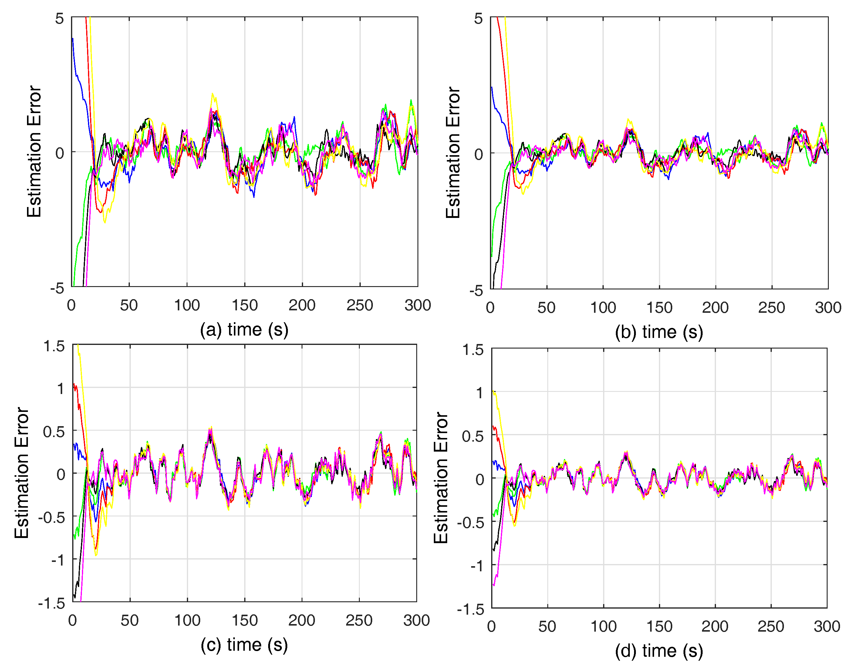
Figure 4.
Upper bound of g for a fixed .
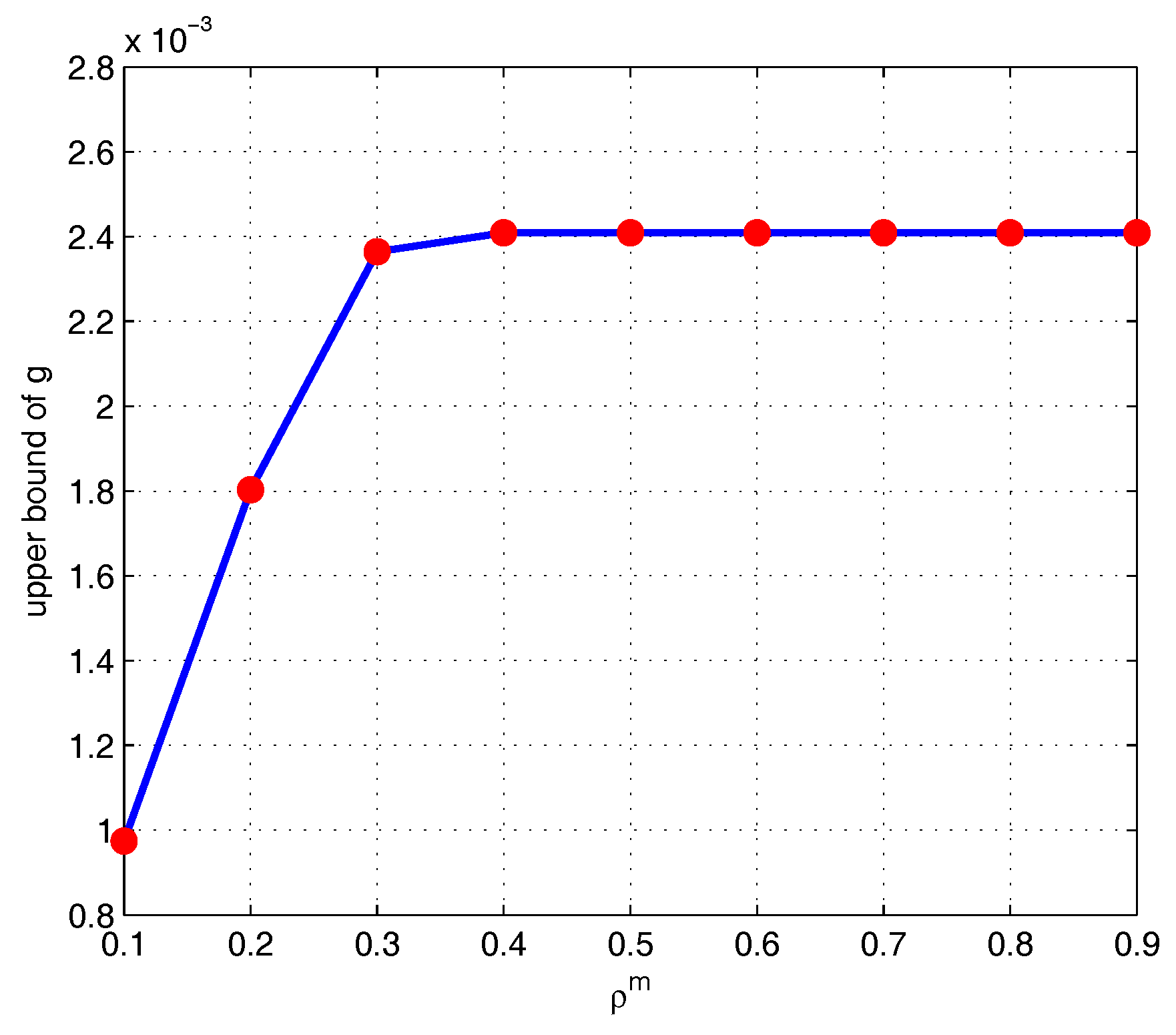
Figure 5.
Upper bound of g for a fixed .
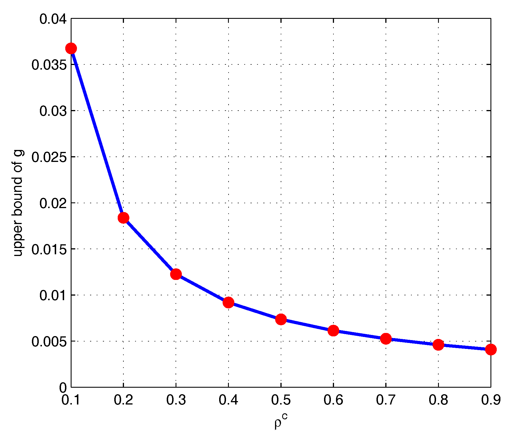
Figure 6.
The triggering sequence.

Figure 7.
Comparison between RSKCF and ETKCF with constraints.

Figure 8.
Communication rate for different .
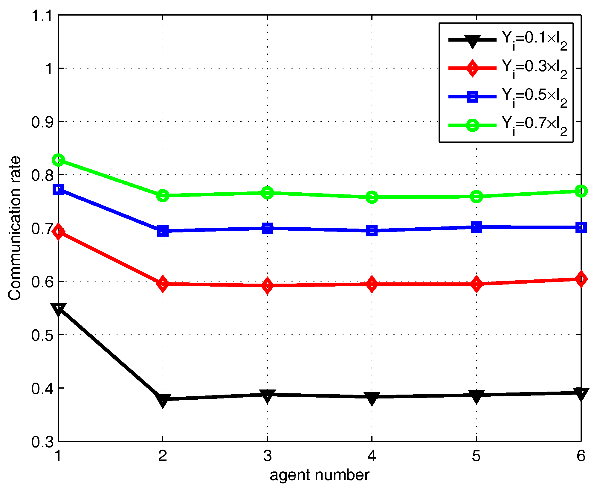
Figure 9.
Network topology of 30 agents.

Figure 10.
Comparison between algorithms 1 and 2 for case 2.
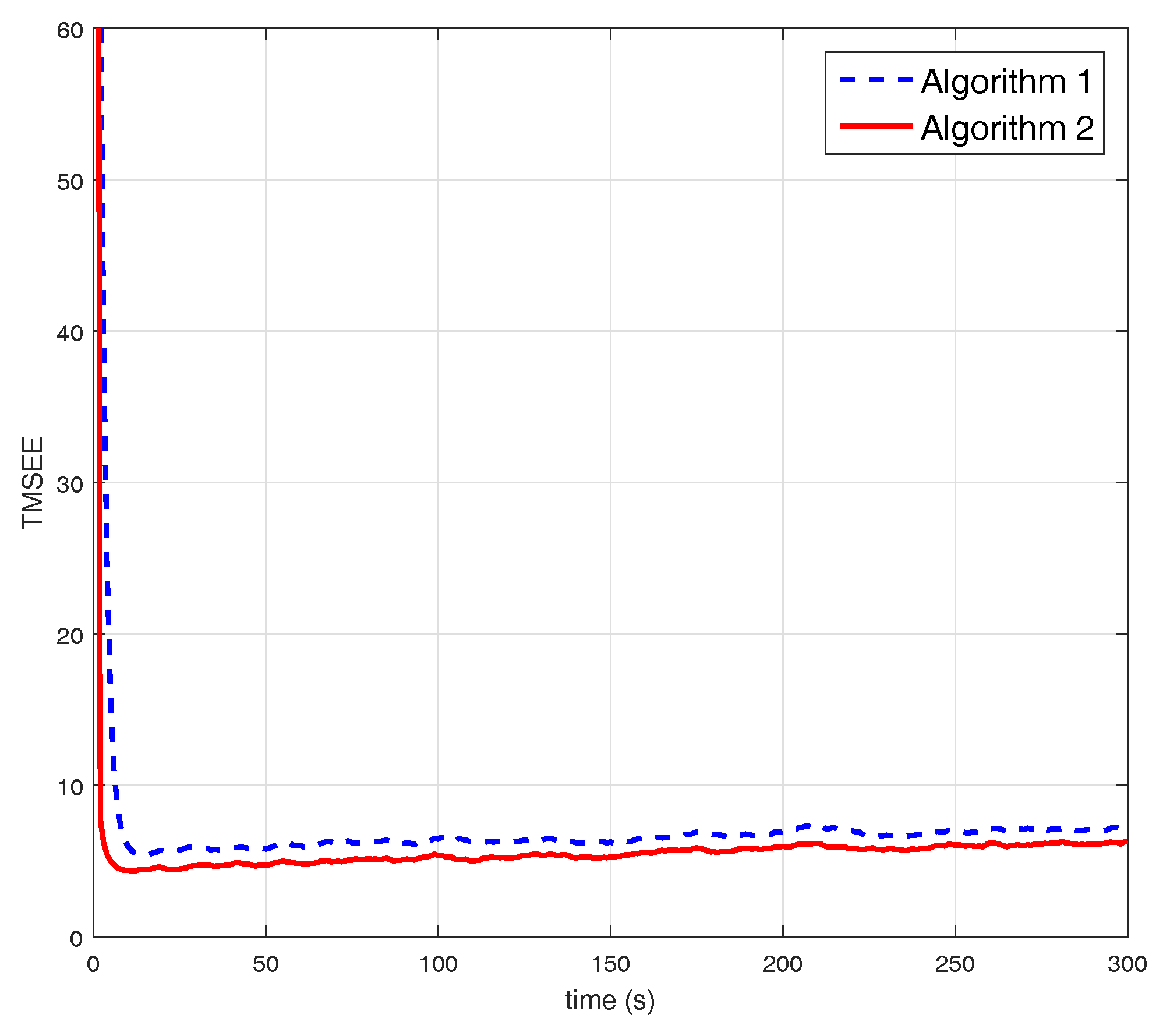
Figure 11.
TMSEE of position and velocity of algorithm 1. (a) TMSEE of position; (b) TMSEE of velocity.
Figure 11.
TMSEE of position and velocity of algorithm 1. (a) TMSEE of position; (b) TMSEE of velocity.

Figure 12.
TMSEE of position and velocity of algorithm 2. (a) TMSEE of position; (b) TMSEE of velocity.
Figure 12.
TMSEE of position and velocity of algorithm 2. (a) TMSEE of position; (b) TMSEE of velocity.

© 2018 by the authors. Licensee MDPI, Basel, Switzerland. This article is an open access article distributed under the terms and conditions of the Creative Commons Attribution (CC BY) license (http://creativecommons.org/licenses/by/4.0/).
Share and Cite
MDPI and ACS Style
Hu, C.; Li, Z.; Lin, H.; He, B.; Liu, G. Distributed State Estimation under State Inequality Constraints with Random Communication over Multi-Agent Networks. Information 2018, 9, 64. https://doi.org/10.3390/info9030064
AMA Style
Hu C, Li Z, Lin H, He B, Liu G. Distributed State Estimation under State Inequality Constraints with Random Communication over Multi-Agent Networks. Information. 2018; 9(3):64. https://doi.org/10.3390/info9030064
Chicago/Turabian StyleHu, Chen, Zhenhua Li, Haoshen Lin, Bing He, and Gang Liu. 2018. "Distributed State Estimation under State Inequality Constraints with Random Communication over Multi-Agent Networks" Information 9, no. 3: 64. https://doi.org/10.3390/info9030064
Note that from the first issue of 2016, this journal uses article numbers instead of page numbers. See further details here.