A New Bi-Directional Projection Model Based on Pythagorean Uncertain Linguistic Variable

School of Management Science and Engineering, Shandong University of Finance and Economics, Jinan 250014, China
*
Author to whom correspondence should be addressed.
Information 2018, 9(5), 104; https://doi.org/10.3390/info9050104
Submission received: 9 April 2018
/
Revised: 20 April 2018
/
Accepted: 21 April 2018
/
Published: 26 April 2018
(This article belongs to the Special Issue Multiple-Criteria Decision-Making (MCDM) Techniques for Business Processes Information Management)
Abstract
:To solve the multi-attribute decision making (MADM) problems with Pythagorean uncertain linguistic variable, an extended bi-directional projection method is proposed. First, we utilize the linguistic scale function to convert uncertain linguistic variable and provide a new projection model, subsequently. Then, to depict the bi-directional projection method, the formative vectors of alternatives and ideal alternatives are defined. Furthermore, a comparative analysis with projection model is conducted to show the superiority of bi-directional projection method. Finally, an example of graduate’s job option is given to demonstrate the effectiveness and feasibility of the proposed method.
1. Introduction
Multi-attribute decision making (MADM) problem is to select the optimal alternative(s) or get the ranking order of all alternatives with multiple attributes. For the complexity of the decision making environment and the limitation of decision makers’ knowledge, vagueness and uncertainty are typical factors we must take into account. To describe the vague and uncertain information accurately, Zadeh [1] proposed the concept of fuzzy set. However, applying fuzzy set to solve decision making problems is confined to the lacking of information. Intuitionistic fuzzy set (IFS) as the extension of fuzzy set, can capture uncertain information more appropriately. Recently, IFS have been extensively applied to MADM area, because the superiority in dealing with vague and uncertain information [2,3,4,5]. Whereas, IFS is difficult to depict vague and uncertain information when the sum of membership degree and non-membership degree is bigger than 1.
To express fuzzy information more effectively, Yager [6] proposed the Pythagorean fuzzy set (PFS) to capture the vague and uncertain information. Different from IFS, the sum of membership degree and non-membership degree of PFS may be bigger than one, but the square sum of them is less than one. As a useful extension of IFS, the PFS can depict the problem which the IFS cannot. For example, if the membership degree and non-membership degree are 0.8 and 0.6, respectively. It is easily to see, the IFS cannot describe this situation because of , but the PFS can effectively solve the issue due to . Since PFS appeared, multi-attribute decision making problems under PFS environment have got a lot of attention, and some research results have been obtained. Du et al. [7] proposed a new score function and a new accurate function of PFS. Liang et al. [8], Liang and Xu [9], and Zhang and Xu [10] extended the TOPSIS (Technique for Order Performance by Similarity to Ideal Solution) method under PFS and hesitant Pythagorean fuzzy set circumstances, respectively. A new closeness index of Pythagorean fuzzy set was proposed by Zhang [11] and the QUALIFLEX (QUALItative FLEXible multiple criteria method) method was extended based on the closeness index subsequently. Ren et al. [12] presented an extended TODIM (An Acronym in Portuguese of Interactive and Multiple Attribute Decision Making) method based on PFS, and made an emulational analysis for the result. Chen [13] proposed a new distance formula for PFS and an extended VIKOR (the Serbian name: Vlsekriterijumska Optimizacijia I Kompromisno Resenje) method was presented based on the distance formula. Following the pioneering work of Yager, Garg [14,15] developed a new relevant coefficient of PFS and an extended accurate function of interval Pythagorean fuzzy set (IPFS), respectively. A new MADM method was proposed by Peng and Dai [16] based on prospect theory and regret theory. Furthermore, Xue et al. [17] defined the concept of entropy of PFS and extended the LINMAP (The Linear Programming Technique for Multidimensional Analysis of Preference) method based on the concept. Liang et al. [18] developed a weighted Pythagorean fuzzy geometric mean operator and extended the projection method based on the geometric mean operator. Peng and Yang [19] proposed an extended ELECTRE (ELimination Et Choice Translating REality) method based on IPFS. The new accurate function and similarity measure of PFS were developed by Zhang [20], respectively.
The projection model can simultaneously consider the angle and distance between two evaluative values [18]. Therefore, the projection model has been widely applied to replace the single distance measure in multi-attribute decision making domain. Tsao and Chen [21] developed a projection model of interval intuitionistic fuzzy set (IIFS) and an extended VIKOR method was proposed based on the projection model. Sun et al. [22] proposed a projection model of hesitant linguistic variable and extended the multi-attributive border approximation area comparison (MABAC) method to hesitant linguistic circumstance. To overcome the drawback of the extant TODIM method, Ji et al. [23] developed a projection-based TODIM method with multi-valued neutrosophic sets (MVNSs). Wu et al. [24] proposed an extended projection model based on hesitant linguistic variable to handle the hospital management problem. Inspired by the advantage of projection model, Liang et al. [25] proposed an extended PROMETHEE (Preference Ranking Organization Method for Enrichment Evaluations) method based on the projection model.
Recently, projection model has been extensively applied to solve the MADM problems due to the advantage of capturing vague and uncertain information. However, projection model cannot effectively get the ranking order when alternatives distribute on the perpendicular bisector of ideal alternatives [26]. Motivated by the drawback of the projection model and the advantage of linguistic variables, we developed an extended bi-directional projection model of Pythagorean uncertain linguistic variables [27]. Our model can not only utilize the advantage of both Pythagorean uncertain linguistic variable and projection models but it can also effectively overcome the defects of the projection model.
This paper is organized as follows. Section 2 presents some basic definitions of IFS, linguistic variables, and the Pythagorean uncertain linguistic variables. In Section 3, we propose a new bi-directional projection model. Comparative analysis of the proposed model and projection model is provided in Section 4 and the MADM Procedures are listed in Section 5. In Section 6, the effectiveness of the proposed method is demonstrated by a practical MADM problem. Finally, Section 7 comes to some conclusions.
2. Preliminaries
Definition 1
[2]. Let be a crisp set, an intuitionistic fuzzy set on can be defined as
where, : and : denote membership function and non-membership function of , respectively, with . denote the hesitation function of .
Definition 2
[28]. Let be linguistic term set, where is a positive integer and denotes an evaluation value of linguistic variable. We call as the uncertain linguistic variable, where and , besides, and are positive integers. denote the upper bound and the lower bound, respectively.
Definition 3
[27]. Let be a fixed set. denote the Pythagorean uncertain linguistic variable on , where function : and : denote membership function and non-membership function of , respectively, with . To expediently depict the evaluation value, we call as the Pythagorean uncertain linguistic number.
Definition 4
[25]. If is a numerical value, then the linguistic scale function can defined as , where . represent the preference of decision maker on the chosen linguistic term .
where denote the sensibility coefficient, and is a monotone increasing function.
Definition 5
Let and be two Pythagorean uncertain linguistic variable on . If we convert and to and via linguistic scale function, then the formative vector of and is computed as
where
Example 1.
Let and be two Pythagorean uncertain linguistic numbers, where , , .
According to Definition 4, we can obtain
Then, the formative vector of and is obtained via (2).
3. Bi-Directional Projection Model
3.1. Projection Model
Let and , which are two Pythagorean uncertain linguistic variables, then the cosine of and is defined as
and denote the modules of and . is linguistic scale function.
Therefore, the projection of and is defined as
Theorem 1
[25]. The cosine of and meets the following several properties
- (1)
- (2)
- (3)
3.2. Bi-Directional Projection Model
Let be an alternative with Pythagorean uncertain linguistic variable information. The positive and negative ideal alternatives are denoted as:
and , respectively, represents the number of alternatives. Then, the formative vectors of and ideal alternatives are denoted as
where
The modules are computed as
The cosine of and is expressed as
The projection value of on and on are calculated as
4. Comparative Analysis of Projection Model and Bi-Directional Projection Model
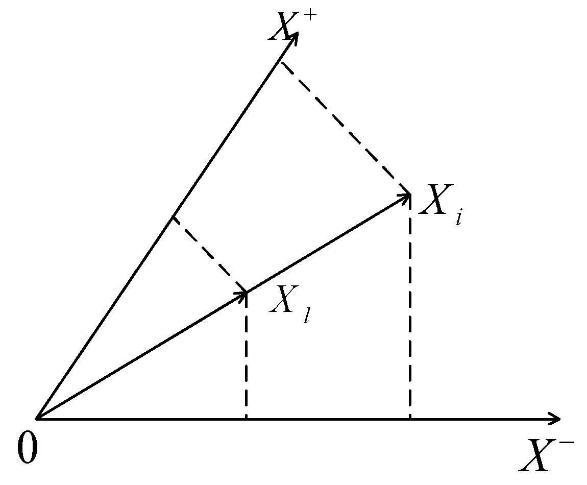
Let and , which are two alternatives with Pythagorean uncertain linguistic variable information, the positive and negative ideal alternatives are defined as and , respectively. The and distribute on the perpendicular bisector of and (shown as Figure 2). We compare the and via projection and bi-directional projection models, respectively.
4.1. Projection Model
- Step 1:
- Compute the projection of and on the positive and negative ideal alternatives via (4).
- Step 2:
- Calculate the closeness degree of and to ideal alternatives, respectively.we can see and because the and distribute on the perpendicular bisector of and . Therefore, , .
Where the closeness degree is ranking indicators. The bigger value of the closeness degree, the better the preference order of the alternatives.
4.2. Bi-Directional Projection Model
- Step 1:
- Compute the formative vector: , , , , respectively.
- Step 2:
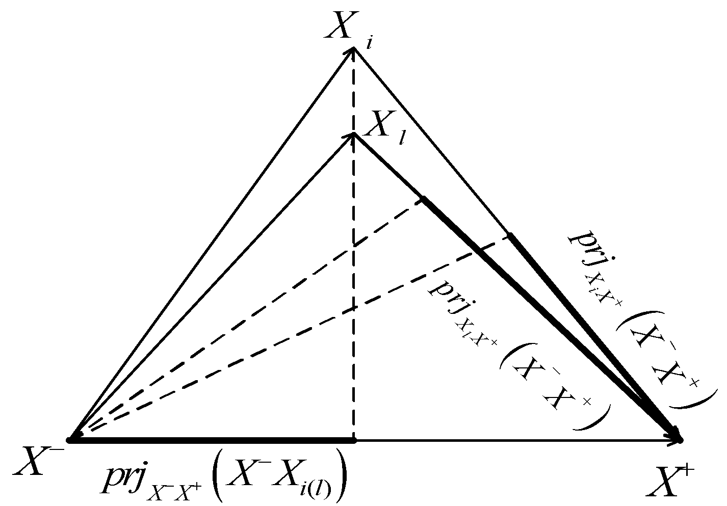
- Calculate the projection value of formative vector and to , denoted as , , and the projection value of formative vector to and , denoted as , , respectively (shown as Figure 3).
- Step 3:
- Compute the closeness degree of and to ideal alternatives.
We can see because and distribute on the perpendicular bisector of ideal alternatives, as shown in Figure 3 . Therefore, , .
From the foregoing analysis, we can know the projection model is difficult to obtain the ranking order of and , when they distribute on the perpendicular bisector of ideal alternatives. Whereas, the bi-directional projection model can remarkably overcome the drawback and get the rational ranking order of and .
5. Decision Making Steps of Bi-Directional Projection Model
To solve certain decision making problems, we propose a new bi-directional projection model based on Pythagorean uncertain linguistic variables. denotes the set of alternatives, the set of attributes are denoted by and the weights are represented by , where , . is the evaluation value of under with Pythagorean uncertain linguistic variable information. The linguistic term set is , and denote the benefit attribute and cost attribute, respectively. In general, the proposed method involves the following steps:
- Step 1:
- Construct the decision making matrix with Pythagorean uncertain linguistic variable information, and normalize the decision matrix.where, is the complement of , and the form of is defined as .
- Step 2:
- Convert the Pythagorean uncertain linguistic variable to Pythagorean uncertain linguistic function via the linguistic scale function.
- Step 3:
- Determine the ideal alternatives and .Where,
- Step 4:
- Compute the formative vector of ideal alternative and via (2).
- Step 5:
- Calculate the projection value of formative vector to , denoted as , and the projection value of formative vector to , denoted as , respectively.
- Step 6:
- Develop a closeness degree formula based on TOPSIS method, and obtain the ranking order of all alternatives via closeness degree.
6. Numerical Example
It is essential to choose the right enterprise for graduates’ future development. In order to provide reasonable employment guidance for graduates, we get the influence factors by questionnaires of 260 college graduates of Shandong province. After eliminating the invalid and incomplete questionnaires, seven main attributes are selected to evaluate the alternative companies according to 210 valid questionnaires. The set of attributes is: {prospects of company, working strength, wage level, personal prospects, social insurance and house funding, professional relevance, geographical}. For the sake of convenience, the set of attributes is denoted by . is cost attribute and the rest are benefit attributes. The detailed guidance process of a graduate is shown as follows: The set of companies are denoted as: and the weights are , where, , which are given by experts, is the evaluation value of under with Pythagorean uncertain linguistic variable information. The linguistic term set is: S = {s0 = extremely bad, s1 = very bad, s2 = bad, s3 = slightly bad, s4 = fair, s5 = good, s6 = slightly good, s7 = very good, s8 = extremely good}. Determine the ranking order of the 10 companies based on bi-directional projection model.
- Step 1:
- Construct the decision making matrix with Pythagorean uncertain linguistic variable information, and normalize the decision matrix.
- Step 2:
- Convert the Pythagorean uncertain linguistic variable to Pythagorean uncertain linguistic function via the linguistic scale function, where , .
- Step 3:
- Determine the positive and negative ideal alternatives and .
- Step 4:
- Compute the formative vector of ideal alternative and via (2).Similarly, we can get the formative vector of ideal alternative and .
- Step 5:
- Calculate the projection value of formative vector to , denoted as , and the projection value of formative vector to , denoted as , respectively.
- Step 6:
- Compute the closeness degree and obtain the ranking order of all alternatives via closeness degree.where,
Therefore, , and is the best company for this graduate.
7. Conclusions
To solve multi-attribute decision making (MADM) problems with Pythagorean uncertain linguistic variables, we proposed an extended bi-directional projection model. The extended model can take the advantages of the Pythagorean uncertain linguistic variable and projection models, and effectively overcome the drawbacks of the single distance measure. The feasibility of the proposed method is demonstrated by the graduates’ job-hunting problem.
The superiority of our bi-directional projection model is that it can consider the angle and distance between two evaluation values simultaneously. Compared with projection model, the proposed model can handle the real-life case of alternatives distribution on the perpendicular bisector of positive and negative ideal alternatives, which made it widely suitable in MADM. However, the proposed method does not consider the psychological risk factors of decision makers in this paper, which will be explored in the future research.
Author Contributions
Huidong Wang conceived the idea; Shifan He and Xiaohong Pan wrote the paper and revised the paper. The authors have read and approved the final manuscript.
Funding
This work was supported by NSFC Foundation under Grant No. 61402260.
Conflicts of Interest
The authors declare no conflict of interest.
References
- Zadeh, L.A. Fuzzy sets. Inf. Control 1965, 8, 338–353. [Google Scholar] [CrossRef]
- Shen, F.; Ma, X.S.; Li, Z.Y.; Cai, D.L. An extended intuitionistic fuzzy TOPSIS method based on a new distance measure with an application to credit risk evaluation. Inf. Sci. 2018, 428, 105–119. [Google Scholar] [CrossRef]
- Qiu, J.D.; Li, L. A new approach for multiple attribute group decision making with interval-valued intuitionistic fuzzy information. Appl. Soft Comput. 2017, 61, 111–121. [Google Scholar] [CrossRef]
- Li, C.D.; Gao, J.L.; Yi, J.Q.; Zhang, G.Q. Analysis and design of functionally weighted single-input-rule-modules connected fuzzy inference systems. IEEE Trans. Fuzzy Syst. 2018, 26, 56–71. [Google Scholar] [CrossRef]
- Cheng, S.H. Autocratic multiattribute group decision making for hotel location selection based on interval-valued intuitionistic fuzzy sets. Inf. Sci. 2018, 427, 77–87. [Google Scholar] [CrossRef]
- Yager, R.R. Pythagorean membership grades in multicriteria decision making. IEEE Trans. Fuzzy Syst. 2014, 22, 958–965. [Google Scholar] [CrossRef]
- Du, Y.Q.; Hu, F.J.; Zafar, W.; Yu, Q.; Zhai, Y. A Novel Method for Multi-attribute Decision Making with Interval-Valued Pythagorean Fuzzy Linguistic Information. Int. J. Intell. Syst. 2017, 32, 1085–1112. [Google Scholar] [CrossRef]
- Liang, D.C.; Xu, Z.S.; Liu, D.; Wu, Y. Method for Three-Way Decisions using Ideal TOPSIS Solutions at Pythagorean Fuzzy Information. Inf. Sci. 2018, 435, 282–295. [Google Scholar] [CrossRef]
- Liang, D.C.; Xu, Z.S. The new extension of TOPSIS method for multiple criteria decision making with hesitant Pythagorean fuzzy sets. Appl. Soft Comput. 2017, 60, 167–179. [Google Scholar] [CrossRef]
- Zhang, X.L.; Xu, Z.S. Extension of TOPSIS to Multiple Criteria Decision Making with Pythagorean Fuzzy Sets. Int. J. Intell. Syst. 2014, 29, 1061–1078. [Google Scholar] [CrossRef]
- Zhang, X.L. Multicriteria Pythagorean fuzzy decision analysis: A hierarchical QUALIFLEX approach with the closeness index-based ranking methods. Inf. Sci. 2016, 330, 104–124. [Google Scholar] [CrossRef]
- Ren, P.J.; Xu, Z.S.; Gou, X.J. Pythagorean fuzzy TODIM approach to multi-criteria decision making. Appl. Soft Comput. 2016, 42, 246–259. [Google Scholar] [CrossRef]
- Chen, T.Y. Remoteness index-based Pythagorean fuzzy VIKOR methods with a generalized distance measure for multiple criteria decision analysis. Inf. Fusion 2018, 41, 129–150. [Google Scholar] [CrossRef]
- Garg, H. A Novel Correlation Coefficients between Pythagorean Fuzzy Sets and Its Applications to Decision-Making Processes. Int. J. Intell. Syst. 2016, 12, 1234–1252. [Google Scholar] [CrossRef]
- Garg, H. A Novel Improved Accuracy Function for Interval Valued Pythagorean Fuzzy Sets and Its Applications in the Decision-Making Process. Int. J. Intell. Syst. 2017, 32, 1247–1260. [Google Scholar] [CrossRef]
- Peng, X.D.; Dai, J.G. Approaches to Pythagorean Fuzzy Stochastic Multi-criteria Decision Making Based on Prospect Theory and Regret Theory with New Distance Measure and Score Function. Int. J. Intell. Syst. 2017, 32, 1187–1214. [Google Scholar] [CrossRef]
- Xue, W.T.; Xu, Z.S.; Zhang, X.L.; Tian, X.L. Pythagorean Fuzzy LINMAP Method Based on the Entropy Theory for Railway Project Investment Decision Making. Int. J. Intell. Syst. 2018, 33, 93–125. [Google Scholar] [CrossRef]
- Liang, D.C.; Xu, Z.S.; Peter, A. Projection Model for Fusing the Information of Pythagorean Fuzzy Multicriteria Group Decision Making Based on Geometric Bonferroni Mean. Int. J. Intell. Syst. 2017, 32, 966–987. [Google Scholar] [CrossRef]
- Peng, X.D.; Yang, Y. Fundamental Properties of Interval-Valued Pythagorean Fuzzy Aggregation Operators. Int. J. Intell. Syst. 2015, 31, 444–487. [Google Scholar] [CrossRef]
- Zhang, X.L. A Novel Approach Based on Similarity Measure for Pythagorean Fuzzy Multiple Criteria Group Decision Making. Int. J. Intell. Syst. 2016, 31, 593–611. [Google Scholar] [CrossRef]
- Tsao, C.Y.; Chen, T.Y. A projection-based compromising method for multiple criteria decision analysis with interval-valued intuitionistic fuzzy information. Appl. Soft Comput. 2016, 45, 207–223. [Google Scholar] [CrossRef]
- Sun, R.X.; Hu, J.H.; Zhou, J.D.; Chen, X. A Hesitant Fuzzy Linguistic Projection-Based MABAC Method for Patients’ Prioritization. Int. J. Fuzzy Syst. 2017, 1, 1–17. [Google Scholar] [CrossRef]
- Ji, P.; Zhang, H.Y.; Wang, J.Q. A projection-based TODIM method under multi-valued neutrosophic environments and its application in personnel selection. Neural Comput. Appl. 2018, 29, 221–234. [Google Scholar] [CrossRef]
- Wu, H.Y.; Xu, Z.S.; Ren, P.J.; Liao, H.C. Hesitant fuzzy linguistic projection model to multi-criteria decision making for hospital decision support systems. Comput. Ind. Eng. 2018, 115, 449–458. [Google Scholar] [CrossRef]
- Liang, R.X.; Wang, J.Q.; Zhang, H.Y. Projection-based PROMETHEE methods based on hesitant fuzzy linguistic term sets. Int. J. Fuzzy Syst. 2017, 1–14. [Google Scholar] [CrossRef]
- Ye, J. Bidirectional projection method for multiple attribute group decision making with neutrosophic numbers. Neural Comput. Appl. 2017, 28, 1021–1029. [Google Scholar] [CrossRef]
- Liu, Z.M.; Liu, P.D.; Liu, W.L. An extended VIKOR method based on Pythagorean uncertain linguistic variable. Control Decis. 2017, 32, 2145–2152. (In Chinese) [Google Scholar]
- Li, D.Q.; Zeng, W.Y.; Li, J.H. Note on uncertain linguistic Bonferroni mean operators and their application to multiple attribute decision making. Appl. Math. Model. 2015, 39, 894–900. [Google Scholar] [CrossRef]
- Liu, X.D.; Zhu, J.J.; Liu, S.F. An bi-directional projection method based on hesitant fuzzy information. Syst. Eng. Theory Pract. 2014, 34, 2637–2644. (In Chinese) [Google Scholar]
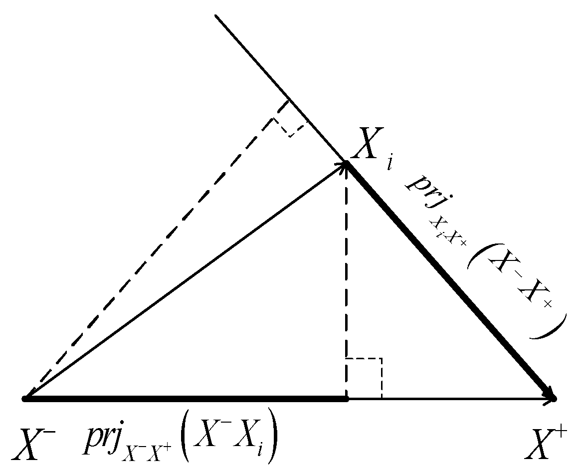
Figure 1.
The graphical representation of and .

Figure 2.
The closeness degree of projection model.

Figure 3.
The closeness degree of bi-directional projection model.

© 2018 by the authors. Licensee MDPI, Basel, Switzerland. This article is an open access article distributed under the terms and conditions of the Creative Commons Attribution (CC BY) license (http://creativecommons.org/licenses/by/4.0/).
Share and Cite
MDPI and ACS Style
Wang, H.; He, S.; Pan, X. A New Bi-Directional Projection Model Based on Pythagorean Uncertain Linguistic Variable. Information 2018, 9, 104. https://doi.org/10.3390/info9050104
AMA Style
Wang H, He S, Pan X. A New Bi-Directional Projection Model Based on Pythagorean Uncertain Linguistic Variable. Information. 2018; 9(5):104. https://doi.org/10.3390/info9050104
Chicago/Turabian StyleWang, Huidong, Shifan He, and Xiaohong Pan. 2018. "A New Bi-Directional Projection Model Based on Pythagorean Uncertain Linguistic Variable" Information 9, no. 5: 104. https://doi.org/10.3390/info9050104
Note that from the first issue of 2016, this journal uses article numbers instead of page numbers. See further details here.