A Novel Rough WASPAS Approach for Supplier Selection in a Company Manufacturing PVC Carpentry Products

Abstract

The decision-making process requires the prior definition and fulfillment of certain factors, especially when it comes to complex areas such as supply chain management. One of the most important items in the initial phase of the supply chain, which strongly influences its further flow, is to decide on the most favorable supplier. In this paper a selection of suppliers in a company producing polyvinyl chloride (PVC) carpentry was made based on the new approach developed in the field of multi-criteria decision making (MCDM). The relative values of the weight coefficients of the criteria are calculated using the rough analytical hierarchical process (AHP) method. The evaluation and ranking of suppliers is carried out using the new rough weighted aggregated sum product assessment (WASPAS) method. In order to determine the stability of the model and the ability to apply the developed rough WASPAS approach, the paper analyzes its sensitivity, which involves changing the value of the coefficient λ in the first part. The second part of the sensitivity analysis relates to the application of different multi-criteria decision-making methods in combination with rough numbers that have been developed in the very recent past. The model presented in the paper is solved by using the following methods: rough Simple Additive Weighting (SAW), rough Evaluation based on Distancefrom Average Solution (EDAS), rough MultiAttributive Border Approximation area Comparison (MABAC), rough Višekriterijumsko kompromisno rangiranje (VIKOR), rough MultiAttributiveIdeal-Real Comparative Analysis (MAIRCA) and rough Multi-objective optimization by ratio analysis plus the full multiplicative form (MULTIMOORA). In addition, in the third part of the sensitivity analysis, the Spearman correlation coefficient (SCC) of the ranks obtained was calculated which confirms the applicability of all the proposed approaches. The proposed rough model allows the evaluation of alternatives despite the imprecision and lack of quantitative information in the information-management process.

1. Introduction

The concept of the supply chain changes over time, but essentially retains its original form; it is growing in importance and, according to Petrović et al. [1], information management and control of the supply chain are the strategic focus of the leading manufacturing companies. This is caused by very rapid changes in the environment in which companies operate, with the globalization of the market and the very high demands of users for whom the high quality of products and services becomes a priority. In today’s supply chains, supply as a subsystem and the choice of an adequate supplier as the most important process in the procurement subsystem are issues of strategic importance for the functioning of production and other companies, and the goal is to model the supply chain in such a way as to provide profitable outputs for all parts of the supply chain and its participants. The basic participants and elements in the supply chain in relation to the time when this concept emerged are still almost the same, with increasing attention paid to the end-user of services and the satisfaction of their requirements and needs. In order for this to be fulfilled and, on the other hand, to generate profit and efficiently carry out a set of activities in the supply chain with as little cost as possible, it is necessary to take into account the method of suppliers’ selection. Since the 1990s, organizational skills were further enhanced according to Monczka et al. [2], and managers began to realize that material inputs from suppliers have a major impact on their ability to respond to the fulfilment of user needs. For this reason, a growing focus has been placed on suppliers as an important factor for the formation of the final product price.

A reliable supplier who performs all his contractual obligations in an adequate way and a smooth flow of goods can be distinguished as the most important goals, on which can largely depend the complete flow of the supply chain and the achievement of the goals of its participants. The choice of suppliers is one of the more important items for supply chain management [3], while managing and developing relationships with suppliers is a critical issue for achieving a competitive advantage [4]. In addition to the aforementioned supply chain processes, information flows and the additional value of material flows are important.

This work has two primary goals, whereby the first objective relates to the possibility of improving the methodology for the treatment of imprecision when it comes to the field of group multiple criteria decision making (MCDM) through the development of the new rough weighted aggregated sum product assessment (WASPAS) approach. The second goal of this paper is to enrich the evaluation methodology and selection of suppliers through a new approach to the treatment of imprecision that is based on rough numbers.

The paper is structured in six sections. In the first section, introductory considerations about the importance and effects of selection the most appropriate suppliers are given. In the second section, a literature review is carried out presenting the application of the WASPAS method in different areas and demonstrating rough sets theory applications. The third section presents the novel rough WASPAS approach with a detailed explanation of each step. The fourth section presents a practical example of selection of a supplier in a polyvinyl chloride (PVC) manufacturing company using a pre-developed approach. The fifth section presents a sensitivity analysis consisting of three parts on the basis of which the stability of the proposed approach is determined. In the same section, in addition to sensitivity analysis, the results obtained are discussed. The sixth section contains concluding remarks.

2. Literature Review

A short literature review is carried out presenting successful applications of the WASPAS method in different precise or uncertain decision-making situations, as well as demonstrating cases of rough sets theory applications in MCDM problems.

2.1. Applications of Weighted Aggregated Sum Product Assessment (WASPAS) Method

The WASPAS method falls within a group of recent MCDM methods. It was developed by Zavadskas et al. in 2012 [5] and so far has been successfully applied in various areas for solving problems of a different nature. Ighravwe and Oke [6] use the WASPAS method for evaluating maintenance performance systems, while Mathew et al. [7] make a selection of an industrial robot. It is also applied to the determination of the location areas of wind farms in [8], while in [9] in combination with factor relationship (FARE) it is applied in hard magnetic material selection. Solving the location problem for the construction of a shopping center was discussed in [10], where this method is also applied. Zavadskas et al. [11] evaluated apartments in residential buildings using the WASPAS method. The following studies in different areas use the WASPAS method [12,13]. The combination of the analytical hierarchical process (AHP) and WASPAS methods is not rare, so a number of publications using AHP for determining the weight values of the criteria and WASPAS for the choice of alternatives can be found in the literature [14,15]. Madić et al. [16] evaluate the machining process with combination of AHP and WASPAS method, while Turskis et al. [17] use the fuzzy form of these methods for construction site selection. A combination of the classic form of these methods is applied to laser cutting in [18]. The combination of Step-wise Weight Assessment Ratio Analysis (SWARA) and WASPAS is used for solar power plant site selection in [19], and in [20] the combination of these two methods is applied in the nanotechnology industry. The integration of the SWARA, Quality function deployment (QFD) and WASPAS methods is proposed in [21] to resolve the selection of suppliers. SWARA was also used to determine the significance of the criteria. This combination is also integrated into [22] where it is used for the selection of staff in tourism. The combination of methods has been also applied in many decision-making problems and environments [23].

The WASPAS method has a number of extensions. Zavadskas et al. in 2015 [24] developed a new WASPAS-G which is a combination of the classic WASPAS method with grey values, while Keshavarz Ghorabaee et al. in 2016 [25] developed a WASPAS method with interval type-2 fuzzy sets to evaluate and select suppliers in the green supply chain. The same approach is combined with the CRiteria Importance Through Inter-criteria Correlation (CRITIC) method used for a third-party logistics (3PL) provider in [26]. A combination of the WASPAS and single-valued neutrosophic set is applied in [27,28]. WASPAS combined with interval-valued intuitionistic fuzzy numbers (IVIF) was developed in [29]. Solving solar-wind power station location problem using the WASPAS method with interval neutrosophic sets was considered in [30].

2.2. Applications of Rough Sets in Multiple Criteria Decision Making (MCDM)

The popularization of rough sets is lately evident and is increasingly used to make decisions in different areas. Song et al. in his paper [31] used a rough Technique for Ordering Preference by Similarity to Ideal Solution (TOPSIS) approach in uncertain environments. Integration of rough AHP and MABAC are proposed in [32], while integration interval rough AHP and interval rough MABAC is proposed in [33] for evaluation of university websites. A rough AHP and rough TOPSIS approach is also used in [34]. Rough numbers in integration with MCDM methods, according Stević et al. [35], give good results, so lately we can notice the popularization of the use of rough numbers [36,37,38]. Besides the AHP method and its rough form, it is also possible to apply rough best worst method (BWM). So far, rough BWM has been applied in several publications. A rough BWM model was applied for determining the importance of the criteria for selecting a wagon for a logistics company in [39]. The evaluation of suppliers can be executed using a new believable rough set approach which was developed in [40] and, according to the authors, it provided good results.

In comparison with other concepts, a novel rough WASPAS approach has some advantages that can be described as follows. The first reason is its advantage in comparison with grey theory. Grey relation analysis provides a well-structured analytical framework for a multi-criteria decision-making process, but it lacks the capability to characterize the subjective perceptions of designers in the evaluation process. Rough set theory may help here, because rough sets can facilitate effective representation of vague information or imprecise data [41]. According to Khoo et al. [42], a very important advantage of using rough set theory to handle vagueness and uncertainty is that it expresses vagueness by means of the boundary region of a set instead of membership function. In addition, the integration of rough numbers in MCDM methods gives the possibility to explore subjective and unclear evaluation of the experts and to avoid assumptions, which is not the case when applying fuzzy theory [35]. According to Hashemkhani Zolfani et al. [10], the main advantage of the WASPAS method is its high degree of reliability. Integration of rough numbers and the WASPAS method with advantages of both concepts presents a very important support in decision-making in everyday conflicting situations.

The purpose of the fuzzy tehnique in the decision making process is to enable the transformation of crisp numbers into fuzzy numbers that show uncertainties in real world systems using the membership function. As opposed to fuzzy sets theory, which requires a subjective approach in determining partial functions and fuzzy set boundaries, rough set theory determines set boundaries based on real values and depends on the degree of certainty of the decision maker. Since rough set theory deals solely with internal knowledge, i.e., operational data, there is no need to rely on assumption models. In other words, when applying rough sets, only the structure of the given data is used instead of various additional/external parameters [43]. Duntsch and Gediga [44] believe that the logic of rough set theory is based solely on data that speak for themselves. When dealing with rough sets, the measurement of uncertainty is based on the vagueness already contained in the data [45]. In this way, the objective indicators contained in the data can be determined. In addition, rough set theory is suitable for application on sets characterized by irrelevant data where the use of statistical methods does not seem appropriate [46].

3. Methods

3.1. Rough Set Theory

In rough set theory, any vague idea can be represented as a couple of exact concepts based on the lower and upper approximations.

Suppose U is the universe which contains all the objects, Y is an arbitrary object of U, R is a set of t classes $\{G_1,G_2,...,G_t\}$ that cover all the objects in U, $R=\{G_1,G_2,...,G_t\}$. If these classes are ordered as $G_1<G_2<...<G_t\}$, then $\forall Y\in U,G_q\in R,1\le q\le t$, by R (Y) we mean the class to which the object belongs, the lower approximation $(\underset{\_}{Apr}(G_q))$, upper approximation $(\overline{Apr}(G_q))$ and boundary region $(\overline{Bnd}(G_q))$ of class $G_q$ are, according to [47], defined as:

$$\underset{\_}{Apr}(G_q)=\{Y\in U/R(Y)\le G_q\}$$

(1)

$$\overline{Apr}(G_q)=\{Y\in U/R(Y)\ge G_q\}$$

(2)

$$Bnd(G_q)=\{Y\in U/R(Y)\ne G_q\}=\{Y\in U/R(Y)>G_q\}\cup \{Y\in U/R(Y)<G_q\}$$

(3)

Then $G_q$ can be shown as rough number $(RN(G_q))$, which is determined by its corresponding lower limit $(\underset{\_}{Lim}(G_q))$ and upper limit $(\overline{Lim}(G_q))$ where:

$$\underset{\_}{Lim}(G_q)=\frac{1}{M_L}{\displaystyle \sum \left\{Y\in \underset{\_}{Apr}(G_q)\right\}R(Y)}$$

(4)

$$\overline{Lim}(G_q)=\frac{1}{M_U}{\displaystyle \sum \left\{Y\in \overline{Apr}(G_q)\right\}R(Y)}$$

(5)

$$RN(G_q)=\left[\underset{\_}{Lim}(G_q),\overline{Lim}(G_q)\right]$$

(6)

where $M_L,M_U$ are the numbers of objects that are contained in $\underset{\_}{Apr}(G_q)$ and $\overline{Apr}(G_q)$, respectively.

3.2. A Novel Rough WASPAS Approach

The WASPAS method [5] represents a relatively new MCDM method, that has been proved to be robust in a number of publications. Bearing in mind all the advantages of using rough theory [48,49] in the MCDM to represent ambiguity, vagueness and uncertainty, the authors have decided in this paper to modify the WASPAS algorithm using rough numbers, which is an original contribution.

The proposed rough WASPAS method consists of the following steps:

Step 1: Formulation of the model, which consists of m alternatives and n criteria.

Step 2: Formation a team of k experts for the evaluation of alternatives according all criteria using the linguistic scale (

Table 1. Linguistic scale for evaluating alternatives depending on the type of criteria [39].

Linguistic Scale	For Criteria of Type Max (Benefit Criteria)	For Criteria of Type Min (Cost Criteria)
Very Poor—VP	1	9
Poor—P	3	7
Medium—M	5	5
Good—G	7	3
Very Good—VG	9	1

).

Step 3: Formation of initial individual matrices based on evaluations made by experts. It is necessary to form as many individual matrices as there are experts. If the model includes e.g., 5 experts it is necessary to form 5 individual matrices.

Step 4: Converting an individual matrix into a group rough matrix. Each individual matrix of experts k₁, k₂, ..., k_n needs to be converted into a rough group matrix (RGM) (1) using Equations (1)–(6):

$$RGM=\left[\begin{array}{c}\left[x_{11}^L,x_{11}^U\right]\\ \left[x_{21}^L,x_{21}^U\right]\\ ⋮\\ \left[x_{m1}^L,x_{m1}^U\right]\end{array}\begin{array}{c}\left[x_{12}^L,x_{12}^U\right]\\ \left[x_{22}^L,x_{22}^U\right]\\ ⋮\\ \left[x_{m2}^L,x_{m2}^U\right]\end{array}\begin{array}{c}\cdots \\ \cdots \\ \ddots \\ \cdots \end{array}\begin{array}{c}\left[x_{1n}^L,x_{1n}^U\right]\\ \left[x_{2n}^L,x_{2n}^U\right]\\ ⋮\\ \left[x_{mn}^L,x_{mn}^U\right]\end{array}\right]$$

(7)

Step 5: In this step it is necessary to normalize the previous matrix using Equations (8) and (9):

$$n_{ij}=\frac{\left[x_{ij}^L;x_{ij}^U\right]}{max\left[x_{ij}^{+L};x_{ij}^{+U}\right]} for C_{1,}{C}_{2,}\dots ,C_n ϵ B$$

(8)

$$n_{ij}=\frac{min\left[x_{ij}^{-L};x_{ij}^{-U}\right]}{\left[x_{ij}^L;x_{ij}^U\right]} for C_{1,}{C}_{2,}\dots ,C_n ϵ C$$

(9)

where $\left[x_{ij}{}^L;x_{ij}{}^U\right]$ denotes the values from the initial rough group matrix, $\max \left[x_{ij}{}^{+L};x_{ij}{}^{+U}\right]$ represent the maximum value of a criterion if the same belongs a set of benefit criteria and $\min \left[x_{ij}{}^{-L};x_{ij}{}^{-U}\right]$ represent minimal value of a criterion if the same belongs a set of cost criteria.

With “⁺“ and “⁻” values are marked in terms of easier recognition of the same criteria that belong to a different type of criteria.

Equations (8) and (9) can simpler be written as:

$$n_{ij}=\left[\frac{x_{ij}^L}{x_{ij}^{+U}}; \frac{x_{ij}^U}{x_{ij}^{+L}}\right] for C_{1,}{C}_{2,}\dots ,C_n ϵ B$$

(10)

$$n_{ij}=\left[\frac{x_{ij}^{-L}}{x_{ij}^U}; \frac{x_{ij}^{-U}}{x_{ij}^L}\right] for C_{1,}{C}_{2,}\dots ,C_n ϵ C$$

(11)

and get a normalized matrix that looks like (12):

$$NM=\left[\begin{array}{c}\left[n_{11}^L,n_{11}^U\right]\\ \left[n_{21}^L,n_{21}^U\right]\\ ⋮\\ \left[n_{m1}^L,n_{m1}^U\right]\end{array}\begin{array}{c}\left[n_{12}^L,n_{12}^U\right]\\ \left[n_{22}^L,n_{22}^U\right]\\ ⋮\\ \left[n_{m2}^L,n_{m2}^U\right]\end{array}\begin{array}{c}\cdots \\ \cdots \\ \ddots \\ \cdots \end{array}\begin{array}{c}\left[n_{1n}^L,n_{1n}^U\right]\\ \left[n_{2n}^L,n_{2n}^U\right]\\ ⋮\\ \left[n_{mn}^L,n_{mn}^U\right]\end{array}\right]$$

(12)

Step 6: Weighting of the normalized matrix by multiplying the previously obtained matrix with weighted values of the criteria (13):

$$\begin{gathered} Vn={\left[v_{ij}^L;v_{ij}^U\right]}_{m\times n} \\ {v}_{ij}^L=w_J^L\times n_{ij}^L, i=1,2,\dots m,j \\ {v}_{ij}^U=w_J^U\times n_{ij}^U, i=1,2,\dots m,j \end{gathered}$$

(13)

where w_J^L is lower limit, and w_J^U is the upper limit of the weight value of the criterion obtained by applying one of the MCDM methods to determine the significance of the criteria.

Step 7: Summing all the values of the alternatives obtained (14):

$$\begin{gathered} Q_i={\left[q_{ij}^L;q_{ij}^U\right]}_{1\times m} \\ {q}_{ij}^L={\displaystyle \sum }_{j=1}^n{v}_{ij}^L; q_{ij}^U={\displaystyle \sum }_{j=1}^n{v}_{ij}^U \end{gathered}$$

(14)

Step 8: Determination of the weighted product model using Equation (15):

$$\begin{gathered} P_i={\left[p_{ij}^L;p_{ij}^U\right]}_{1\times m} \\ {p}_{ij}^L={\displaystyle \prod }_{j=1}^n{\left(v_{ij}^L\right)}^{w_J^L} \\ {p}_{ij}^U={\displaystyle \prod }_{j=1}^n{\left(v_{ij}^U\right)}^{w_J^U} \end{gathered}$$

(15)

Step 9: Determination of the relative values of the alternative A_i (16):

$$\begin{gathered} A_i={\left[a_{ij}^L;a_{ij}^U\right]}_{1xm} \\ {A}_i=\lambda \times Q_i+\left(1-\lambda \right)\times P_i \end{gathered}$$

(16)

Coefficient $\lambda$ can be crisp values in range 0, 0.1, 0.2,….1.0, but it is recommended to apply the Equation (17) for its calculation:

$$\lambda =0.5+\frac{\sum P_i}{\sum Q_i+\sum P_i}=0.5+\frac{\sum \left[p_{ij}^L;p_{ij}^U\right]}{\sum \left[q_{ij}^L;q_{ij}^U\right]+\sum \left[p_{ij}^L;p_{ij}^U\right]}$$

(17)

Step 10: Ranking the alternatives. The highest value of the alternative marks the best ranked, while the smallest value reflects the worst alternative.

4. Supplier Selection in a Company Manufacturing Polyvinyl Chloride (PVC) Carpentry

Supplier selection in the company manufacturing PVC carpentry was carried out on the basis of the combination of nine quantitative and qualitative criteria: quality of the material, price of the material, certification of the products, delivery time, reputation, volume discounts, warranty period, reliability, and the method of payments. The second and the fourth criteria (the price of the material and delivery time) are the Expenses criteria (type min), while the others are the Benefit criteria (type max). Criteria used in this paper were selected and verified through two-year research related to the evaluation of suppliers in the manufacturing companies of the supply chain presented in [50]. The market is filled with a large number of manufacturers of PVC carpentry products which need an adequate supplier for ensuring the low cost of a product and a good position in the market. In the research, six suppliers (alternatives) were selected from different countries which were evaluated using a developed rough model. In this study, a group of five experts took part in the assessment process. After the interview with the experts, the collected data were processed, and the aggregation of the expert opinion was obtained.

The rough AHP method [51] was used to determine the weight values of the criteria with the following calculation procedure:

Step 1: After the experts’ evaluation of criteria, by applying Saaty’s scale, five matrices of comparison were constructed in criteria sets (

Table 2. Expert evaluation of the criteria.

E1										E2
	C1	C2	C3	C4	C5	C6	C7	C8	C9	C1	C2	C3	C4	C5	C6	C7	C8	C9
C1	1.00	7.00	2.00	5.00	6.00	4.00	3.00	3.00	8.00	1.00	8.00	2.00	6.00	6.00	4.00	5.00	3.00	9.00
C2	0.14	1.00	0.17	0.33	0.50	0.33	0.25	0.17	2.00	0.13	1.00	0.14	0.25	0.50	0.33	0.25	0.17	2.00
C3	0.50	6.00	1.00	4.00	5.00	6.00	2.00	2.00	7.00	0.50	7.00	1.00	4.00	5.00	6.00	2.00	2.00	7.00
C4	0.20	3.00	0.25	1.00	2.00	0.50	0.33	0.25	4.00	0.20	4.00	0.25	1.00	2.00	0.50	0.33	0.25	4.00
C5	0.17	2.00	0.20	0.50	1.00	0.33	0.25	0.20	3.00	0.17	2.00	0.20	0.50	1.00	0.33	0.25	0.20	3.00
C6	0.25	3.00	0.17	2.00	3.00	1.00	0.50	0.33	5.00	0.17	3.00	0.17	2.00	3.00	1.00	0.50	0.33	5.00
C7	0.33	4.00	0.50	3.00	4.00	2.00	1.00	0.50	5.00	0.20	4.00	0.50	3.00	4.00	2.00	1.00	0.50	5.00
C8	0.33	6.00	0.50	4.00	5.00	3.00	2.00	1.00	6.00	0.33	6.00	0.50	4.00	5.00	3.00	2.00	1.00	6.00
C9	0.13	0.50	0.14	0.25	0.33	0.20	0.20	0.17	1.00	0.11	0.50	0.14	0.25	0.33	0.20	0.20	0.17	1.00
E3										E4
	C1	C2	C3	C4	C5	C6	C7	C8	C9	C1	C2	C3	C4	C5	C6	C7	C8	C9
C1	1.00	8.00	1.00	6.00	6.00	4.00	5.00	3.00	8.00	1.00	6.00	0.50	4.00	5.00	4.00	2.00	2.00	7.00
C2	0.13	1.00	0.14	0.25	0.50	0.33	0.25	0.17	1.00	0.17	1.00	0.14	0.33	0.50	0.33	0.25	0.17	2.00
C3	1.00	7.00	1.00	6.00	6.00	4.00	5.00	3.00	8.00	2.00	7.00	1.00	5.00	6.00	6.00	3.00	3.00	8.00
C4	0.20	4.00	0.20	1.00	2.00	0.50	0.33	0.25	4.00	0.25	3.00	0.20	1.00	2.00	0.50	0.33	0.25	4.00
C5	0.17	2.00	0.17	0.50	1.00	0.33	0.25	0.20	3.00	0.20	2.00	0.17	0.50	1.00	0.33	0.25	0.20	3.00
C6	0.17	3.00	0.17	2.00	3.00	1.00	0.50	0.33	5.00	0.25	3.00	0.17	2.00	3.00	1.00	0.50	0.33	5.00
C7	0.20	4.00	0.20	3.00	4.00	2.00	1.00	0.50	5.00	0.50	4.00	0.33	3.00	4.00	2.00	1.00	0.50	5.00
C8	0.33	6.00	0.33	4.00	5.00	3.00	2.00	1.00	6.00	0.50	6.00	0.33	4.00	5.00	3.00	2.00	1.00	6.00
C9	0.13	1.00	0.13	0.25	0.33	0.20	0.20	0.17	1.00	0.14	0.50	0.13	0.25	0.33	0.20	0.20	0.17	1.00
E5
	C1	C2	C3	C4	C5	C6	C7	C8	C9
C1	1.00	6.00	0.50	4.00	5.00	4.00	2.00	2.00	7.00
C2	0.17	1.00	0.14	0.33	0.50	0.33	0.25	0.17	2.00
C3	2.00	7.00	1.00	5.00	6.00	6.00	3.00	3.00	8.00
C4	0.25	3.00	0.20	1.00	2.00	0.50	0.33	0.25	4.00
C5	0.20	2.00	0.17	0.50	1.00	0.33	0.25	0.25	3.00
C6	0.25	3.00	0.17	2.00	3.00	1.00	0.50	0.50	5.00
C7	0.50	4.00	0.33	3.00	4.00	2.00	1.00	1.00	5.00
C8	0.50	6.00	0.33	4.00	4.00	2.00	1.00	1.00	5.00
C9	0.14	0.50	0.13	0.25	0.33	0.20	0.20	0.20	1.00

).

By applying Expressions (1)–(6), each of presented sequences is transformed in rough sequence. So, for the sequence ${\tilde{x}}_{12}=\left\{7,8,8,6,6\right\}$ we get:

$$\begin{gathered} \underset{\_}{Lim}\left(6\right)=6.00,\hspace{1em}\overline{Lim}\left(6\right)=\frac{1}{5}\left(7+8+8+6+6\right)=7.00 \\ \underset{\_}{Lim}\left(7\right)=\frac{1}{3}\left(7+6+6\right)=6.33,\hspace{1em}\overline{Lim}\left(7\right)=\frac{1}{3}\left(7+8+8\right)=7.67 \\ \underset{\_}{Lim}\left(8\right)=\frac{1}{5}\left(7+8+8+6+6\right)=7.00,\hspace{1em}\overline{Lim}\left(8\right)=8.00 \\ RN(x_{12}^1)=\left[6.33;7.67\right];RN(x_{12}^2)=RN(x_{12}^3)=\left[7.00;8.00\right]; RN(x_{12}^4)=RN(x_{12}^5)=\left[6.00;7.00\right] \\ {x}_{12}^L=\frac{x_{12}^1+x_{12}^2+x_{12}^s+x_{12}^4+x_{12}^5}{S}=\frac{6.33+7.00+7.00+6.00+6.00}{5}=6.47 \\ {x}_{12}^U=\frac{x_{12}^1+x_{12}^2+x_{12}^s+x_{12}^4+x_{12}^5}{S}=\frac{7.67+8.00+8.00+7.00+7.00}{5}=7.53 \end{gathered}$$

After formation of the group rough matrix shown in

Table 3. Group rough matrix.

	C1	C2	C3	C4	C5	C6	C7	C8	C9
C1	[1, 1]	[6.47, 7.53]	[0.81, 1.61]	[4.47, 5.53]	[5.36, 5.84]	[4, 4]	[2.63, 4.23]	[2.36, 2.84]	[7.36, 8.25]
C2	[0.14, 0.16]	[1, 1]	[0.14, 0.15]	[0.28, 0.32]	[0.5, 0.5]	[0.33, 0.33]	[0.25, 0.25]	[0.17, 0.17]	[1.64, 1.96]
C3	[0.81, 1.61]	[6.64, 6.96]	[1, 1]	[4.36, 5.25]	[5.36, 5.84]	[5.28, 5.92]	[2.4, 3.67]	[2.36, 2.84]	[7.36, 7.84]
C4	[0.21, 0.23]	[3.16, 3.64]	[0.21, 0.23]	[1, 1]	[2, 2]	[0.5, 0.5]	[0.33, 0.33]	[0.25, 0.25]	[4, 4]
C5	[0.17, 0.19]	[2, 2]	[0.17, 0.19]	[0.5, 0.5]	[1, 1]	[0.33, 0.33]	[0.25, 0.25]	[0.2, 0.22]	[3, 3]
C6	[0.2, 0.24]	[3, 3]	[0.17, 0.17]	[2, 2]	[3, 3]	[1, 1]	[0.5, 0.5]	[0.34, 0.4]	[5, 5]
C7	[0.27, 0.43]	[4, 4]	[0.3, 0.44]	[3, 3]	[4, 4]	[2, 2]	[1, 1]	[0.52, 0.68]	[5, 5]
C8	[0.36, 0.44]	[6, 6]	[0.36, 0.44]	[4, 4]	[4.64, 4.96]	[2.64, 2,96]	[1.64, 1,96]	[1, 1]	[5.64, 5.96]
C9	[0.12, 0.14]	[0.52, 0.68]	[0.13, 0.14]	[0.25, 0.25]	[0.33, 0.33]	[0.2, 0.2]	[0.2, 0.2]	[0.17, 0.18]	[1, 1]

, it is necessary to calculate the geometric middle of the upper and lower limits of the group matrix of the criteria. From the obtained matrix maximum value, the upper limit is chosen, and all other values are divided by that. In that way, we obtain the final values of the criteria weight:

$$w_j\left[\begin{array}{c}\left[0.803,0.992\right]\\ \left[0.090, 0.095\right]\\ \left[0.819, 1.000\right]\\ \left[0.187, 0.194\right]\\ \left[0.127, 0.132\right]\\ \left[0.245, 0.254\right]\\ \left[0,367, 0,416\right]\\ \left[0.505, 0.552\right]\\ \left[0.067, 0.071\right]\end{array}\right]$$

(18)

After obtaining the weight of the criteria, the expert team performed an evaluation of the alternatives (

Table 4. Evaluation of the alternatives based on the criteria of five experts.

	A1					A2					A3
	E1	E2	E3	E4	E5	E1	E2	E3	E4	E5	E1	E2	E3	E4	E5
C1	7	9	5	5	7	7	7	3	5	7	5	3	5	7	5
C2	1	1	1	3	1	3	3	5	1	3	7	9	3	5	7
C3	3	3	1	3	1	7	9	5	5	7	7	7	3	5	5
C4	9	7	7	9	9	9	5	5	7	9	5	1	7	7	5
C5	1	9	1	3	3	3	7	3	5	5	7	5	3	5	9
C6	3	7	3	3	7	5	7	5	3	7	7	5	3	5	9
C7	5	5	3	3	5	5	3	5	1	5	7	7	5	3	7
C8	3	5	1	1	7	5	7	3	3	9	5	5	5	3	9
C9	3	7	3	1	7	3	5	1	3	5	7	5	3	5	7
	A4					A5					A6
C1	5	3	7	7	5	5	3	5	7	5	3	5	3	5	5
C2	3	7	5	3	5	9	9	5	5	9	7	7	7	5	7
C3	3	3	1	3	1	9	9	5	7	7	7	9	3	5	7
C4	5	3	7	5	5	3	1	5	5	1	3	3	3	5	3
C5	7	5	5	5	9	7	5	9	7	9	5	5	3	3	5
C6	3	3	5	3	9	5	5	3	7	5	3	5	3	5	9
C7	9	7	5	3	9	9	7	5	3	9	3	3	1	3	3
C8	5	5	3	3	7	5	5	5	5	7	3	5	3	5	5
C9	5	5	5	3	9	7	5	5	5	9	3	1	5	5	3

).

After the first two steps of the rough WASPAS method which imply the setting of a model by choosing the criteria and alternatives in the first step and determining the expert assessment in the second step (Table 2), it is necessary to convert all the individual matrices from the third step into a group rough matrix, which is the fourth step.

Converting individual matrices into rough matrices is executed in the same way as was the case in determining the weight values of the criteria. The example of the group matrix elements evaluation is presented in

Table 5. Group rough matrix.

	C1	C2	C3	C4	C5	C6	C7	C8	C9
A1	[5.72, 7.51]	[1.08, 1.72]	[1.72, 2.68]	[7.72, 8.68]	[1.88, 5.16]	[3.64, 5.56]	[3.72, 4.68]	[1.91, 4.96]	[2.81, 5.64]
A2	[4.88, 6.66]	[2.3, 3.7]	[5.72, 7.51]	[5.93, 8.07]	[3.72, 5.51]	[4.49, 6.28]	[2.88, 4.66]	[3.91, 6.96]	[2.49, 4.28]
A3	[4.3, 5.7]	[4.84, 7.51]	[4.49, 6.28]	[3.67, 6.2]	[4.49, 7.16]	[4.49, 7.16]	[4.88, 6.66]	[4.38, 6.48]	[4.49, 6.28]
A4	[4.49, 6.28]	[3.72, 5.51]	[1.72, 2.68]	[4.3, 5.7]	[5.34, 7.12]	[3.42, 5.96]	[5.04, 8.09]	[3.72, 5.51]	[4.38, 6.48]
A5	[4.3, 5.7]	[6.44, 8.36]	[6.49, 8.28]	[1.93, 4.07]	[6.49, 8.28]	[4.3, 5.7]	[5.04, 8.09]	[5.08, 5.72]	[5.34, 7.12]
A6	[3.72, 4.68]	[6.28, 6.92]	[4.84, 7.51]	[3.08, 3.72]	[3.72, 4.68]	[3.8, 6.33]	[2.28, 2.92]	[3.72, 4.68]	[2.49, 4.28]

.

$$\begin{gathered} {\tilde{x}}_{11}=\left\{7,9,5,5,7\right\} \\ \underset{\_}{Lim}\left(5\right)=5.00,\hspace{1em}\overline{Lim}\left(5\right)=\frac{1}{5}\left(7+9+5+5+7\right)=6.60 \\ \underset{\_}{Lim}\left(7\right)=\frac{1}{4}\left(7+5+5+7\right)=6.00,\hspace{1em}\overline{Lim}\left(7\right)=\frac{1}{3}\left(7+9+7\right)=7.67 \\ \underset{\_}{Lim}\left(9\right)=\frac{1}{5}\left(7+9+5+5+7\right)=6.60,\hspace{1em}\overline{Lim}\left(9\right)=9.00 \\ RN(x_{11}^1)=RN(x_{11}^5)=\left[6.00;7.67\right];RN(x_{11}^2)=\left[6.60;9.00\right]; RN(x_{11}^3)= RN(x_{11}^4)=\left[5.00;6.60\right] \\ {x}_{11}^L=\frac{x_{11}^1+x_{11}^2+x_{11}^s+x_{11}^4+x_{11}^5}{S}=\frac{6.00+6.60+5.00+5.00+6.00}{5}=5.72 \\ {x}_{11}^U=\frac{x_{11}^1+x_{11}^2+x_{11}^s+x_{11}^4+x_{11}^5}{S}=\frac{7.67+9.00+6.60+6.60+7.67}{5}=7.51 \end{gathered}$$

(19)

In the fifth step, it is necessary to normalize a rough group matrix using Equations (8) and (9) (

Table 6. Normalized matrix.

	C1	C2	C3	C4	C5	C6	C7	C8	C9
A1	[0.76, 1.31]	[0.63, 1.59]	[0.21, 0.41]	[0.22, 0.48]	[0.23, 0.8]	[0.51, 1.24]	[0.46, 0.93]	[0.27, 0.98]	[0.39, 1.06]
A2	[0.65, 1.16]	[0.29, 0.75]	[0.69, 1.16]	[0.24, 0.63]	[0.45, 0.85]	[0.63, 1.4]	[0.36, 0.92]	[0.56, 1.37]	[0.35, 0.8]
A3	[0.57, 1]	[0.14, 0.36]	[0.54, 0.97]	[0.31, 1.01]	[0.54, 1.1]	[0.63, 1.59]	[0.6, 1.32]	[0.63, 1.28]	[0.63, 1.18]
A4	[0.6, 1.1]	[0.2, 0.46]	[0.21, 0.41]	[0.34, 0.87]	[0.64, 1.1]	[0.48, 1.33]	[0.62, 1.61]	[0.53, 1.08]	[0.62, 1.21]
A5	[0.57, 1]	[0.13, 0.27]	[0.78, 1.28]	[0.47, 1.93]	[0.78, 1.28]	[0.6, 1.27]	[0.62, 1.61]	[0.73, 1.13]	[0.75, 1.33]
A6	[0.5, 0.82]	[0.16, 0.27]	[0.58, 1.16]	[0.52, 1.21]	[0.45, 0.72]	[0.53, 1.41]	[0.28, 0.58]	[0.53, 0.92]	[0.35, 0.8]

) in the following way:

Normalization of the group matrix elements for benefit criteria was carried out in the following way:

$$n_{11}=\left[\frac{x_{ij}^L}{x_{ij}^{+U}}; \frac{x_{ij}^U}{x_{ij}^{+L}}\right]=\left[\frac{4.88}{7.51}; \frac{6.66}{5.72}\right]\to n_{11}=\left[0.65; 1.16\right]$$

(20)

and for the cost criteria:

$$n_{22}=\left[\frac{x_{ij}^{-L}}{x_{ij}^U}; \frac{x_{ij}^{-U}}{x_{ij}^L}\right]=\left[\frac{1.08}{3.70}; \frac{1.72}{2.30}\right]\to n_{22}=\left[0.29; 0.75\right]$$

Step 6: Weighting of the normalized matrix multiplying the previously obtained matrix by the weighted values of the criteria using Equation (13) (

Table 7. Weighted normalized matrix.

	C1	C2	C3	C4	C5	C6	C7	C8	C9
A1	[0.61, 1.3]	[0.06, 0.15]	[0.17, 0.41]	[0.04, 0.09]	[0.03, 0.1]	[0.12, 0.31]	[0.17, 0.39]	[0.14, 0.54]	[0.03, 0.08]
A2	[0.52, 1.16]	[0.03, 0.07]	[0.57, 1.16]	[0.04, 0.12]	[0.06, 0.11]	[0.15, 0.36]	[0.13, 0.38]	[0.28, 0.76]	[0.02, 0.06]
A3	[0.46, 0.99]	[0.01, 0.03]	[0.44, 0.97]	[0.06, 0.2]	[0.07, 0.15]	[0.15, 0.41]	[0.22, 0.55]	[0.32, 0.7]	[0.04, 0.08]
A4	[0.48, 1.09]	[0.02, 0.04]	[0.17, 0.41]	[0.06, 0.17]	[0.08, 0.14]	[0.12, 0.34]	[0.23, 0.67]	[0.27, 0.6]	[0.04, 0.09]
A5	[0.46, 0.99]	[0.01, 0.03]	[0.64, 1.28]	[0.09, 0.37]	[0.1, 0.17]	[0.15, 0.32]	[0.23, 0.67]	[0.37, 0.62]	[0.05, 0.1]
A6	[0.4, 0.81]	[0.01, 0.03]	[0.48, 1.16]	[0.1, 0.23]	[0.06, 0.09]	[0.13, 0.36]	[0.1, 0.24]	[0.27, 0.51]	[0.02, 0.06]

):

$$v_{13}^L=\left[ w_3^L\times n_{13}^L;w_3^U\times n_{13}^U\right]= \left[0.82\times 0.21; 1.00\times 0.41\right]\to v_{13}^L=\left[0,17;0.41\right]$$

Step 7: Summing all the values of the alternatives obtained (summing by rows) (14):

$$\begin{gathered} Q_i={\left[q_{ij}^L;q_{ij}^U\right]}_{1\times m} \\ {q}_{ij}^L={\displaystyle \sum }_{j=1}^n{v}_{ij}^L; q_{ij}^U={\displaystyle \sum }_{j=1}^n{v}_{ij}^U \\ {q}_{11}^L=\left[0.61+0.06+0.17+0.04+0.03+0.12+0.17+0.14+0.03\right]=1.37 \\ {q}_{11}^U=\left[1.3+0.15+0.41+0.09+0.1+0.31+0.39+0.54+0.08\right]=3.38 \\ WSM=\left[\begin{array}{c}\left[1.37,3.38\right]\\ \left[1.81,4.17\right]\\ \left[1.78, 4.08\right]\\ \left[1.47, 3.55\right]\\ \left[2.10, 4.54\right]\\ \left[1.57, 3.49\right]\end{array}\right] \end{gathered}$$

(21)

Step 8: Determination of the weighted product model using Equation (15):

$$\begin{gathered} P_i={\left[p_{ij}^L;p_{ij}^U\right]}_{1\times m} \\ {p}_{ij}^L={\displaystyle \prod }_{j=1}^n{\left(v_{ij}^L\right)}^{w_J^L} \\ {p}_{ij}^U={\displaystyle \prod }_{j=1}^n{\left(v_{ij}^U\right)}^{w_J^U} \\ {p}_{11}^L=\left[\left({0.61}^{0.80}\right)\times \left({0.06}^{0.09}\right)\times \left({0.17}^{0.82}\right)\times \left({0.04}^{0.19}\right)\times \left({0.03}^{0.13}\right)\times \left({0.12}^{0.24}\right)\times \left({0.17}^{0.37}\right)\times \left({0.14}^{0.50}\right)\times \left({0.03}^{0.07}\right)\right]=0.004 \\ {p}_{11}^u=\left[\left({1.30}^{0.99}\right)\times \left({0.15}^{0.09}\right)\times \left({0.41}^{1.00}\right)\times \left({0.09}^{0.19}\right)\times \left({0.1}^{0.13}\right)\times \left({0.31}^{0.25}\right)\times \left({0.39}^{0.42}\right)\times \left({0.54}^{0.55}\right)\times \left({0.08}^{0.07}\right)\right]=0.063 \\ WPM=\left[\begin{array}{c}\left[0.004,0.063\right]\\ \left[0.013,0.187\right]\\ \left[0.013, 0.168\right]\\ \left[0.006, 0.074\right]\\ \left[0.021, 0.240\right]\\ \left[0.008, 0.088\right]\end{array}\right] \end{gathered}$$

Step 9: Determination of the relative values of the alternative A_i (Equation (16)):

$$\begin{gathered} A_i={\left[a_{ij}^L;a_{ij}^U\right]}_{1xm} \\ {A}_i=\lambda \times Q_i+\left(1-\lambda \right)\times P_i \end{gathered}$$

(22)

Coeficient $\lambda$ can be in the range of 0, 0.1, 0.2, …, 1.0.

However, it is recommended to apply Equation (17) for its calculation:

$$\lambda =0.5+\frac{\sum P_i}{\sum Q_i+\sum P_i}=0.5+\frac{\left[0.065,0.820\right]}{\left[10.087,23.203\right]+\left[0.065,0.820\right]}=\left[0.503,0.581\right]$$

Table 8. Determining the relative values of the alternatives and their ranking.

	λ × Qi	(1 − λ) × Pi	Ai	Crisp Ai	Rank
A1	[0.687, 1.963]	[0.002, 0.031]	[0.689, 1.995]	1.342	6
A2	[0.908, 2.422]	[0.005, 0.093]	[0.914, 2.515	1.714	2
A3	[0.894, 2.367]	[0.005, 0.083]	[0.899, 2.450]	1.675	3
A4	[0.739, 2.061]	[0.002, 0.037]	[0.741, 2.098]	1.419	5
A5	[1.053, 2.636]	[0.009, 0.119]	[1.063, 2.755	1.909	1
A6	[0.790, 2.026]	[0.004, 0.044]	[0.793, 2.070]	1.432	4

shows the calculations of Equation (16). At first it is necessary to calculate the product of the coefficient λ with the values of the Qi matrix from the 7th step. After that, it is necessary to detract a rough number of the coefficient λ from one (1) and multiply it with the values of the P_i matrix from the 8th step. In addition, Table 8 shows rough values for each alternative, their crisp number and ranking.

After applying the previous 1–9 steps of the rough WASPAS method, in the last, 10th step it is necessary to perform the ranking of alternatives. The highest value represents the best alternative, which in this case is alternative A₅, while the worst alternative is alternative A₁.

5. Sensitivity Analysis

The sensitivity analysis performed in this paper consists of three parts. In step 9, it is indicated that besides Equation (17) which is recommended for the calculation of the coefficient λ, this can also have a crisp value in the range of 0.1, 0.2, 0.3, ..., 1.0. Therefore, in the first part of the sensitivity analysis, a change in the coefficient λ was made, which is shown in

Table 9. Relative values of the alternatives depending on the value of the coefficient λ.

	λ = 0	λ = 0.1	λ = 0.2	λ = 0.3	λ = 0.4	λ = 0.5	λ = 0.6	λ = 0.7	λ = 0.8	λ = 0.9	λ = 1.0
A1	0.033	0.267	0.501	0.735	0.969	1.203	1.437	1.671	1.905	2.139	2.374
A2	0.100	0.389	0.678	0.967	1.255	1.544	1.833	2.122	2.411	2.699	2.989
A3	0.090	0.374	0.658	0.942	1.225	1.509	1.792	2.076	2.359	2.643	2.927
A4	0.040	0.287	0.534	0.781	1.028	1.275	1.521	1.768	2.015	2.262	2.509
A5	0.131	0.449	0.768	1.086	1.405	1.724	2.042	2.361	2.680	2.998	3.317
A6	0.048	0.296	0.545	0.793	1.041	1.289	1.537	1.785	2.034	2.282	2.530

.

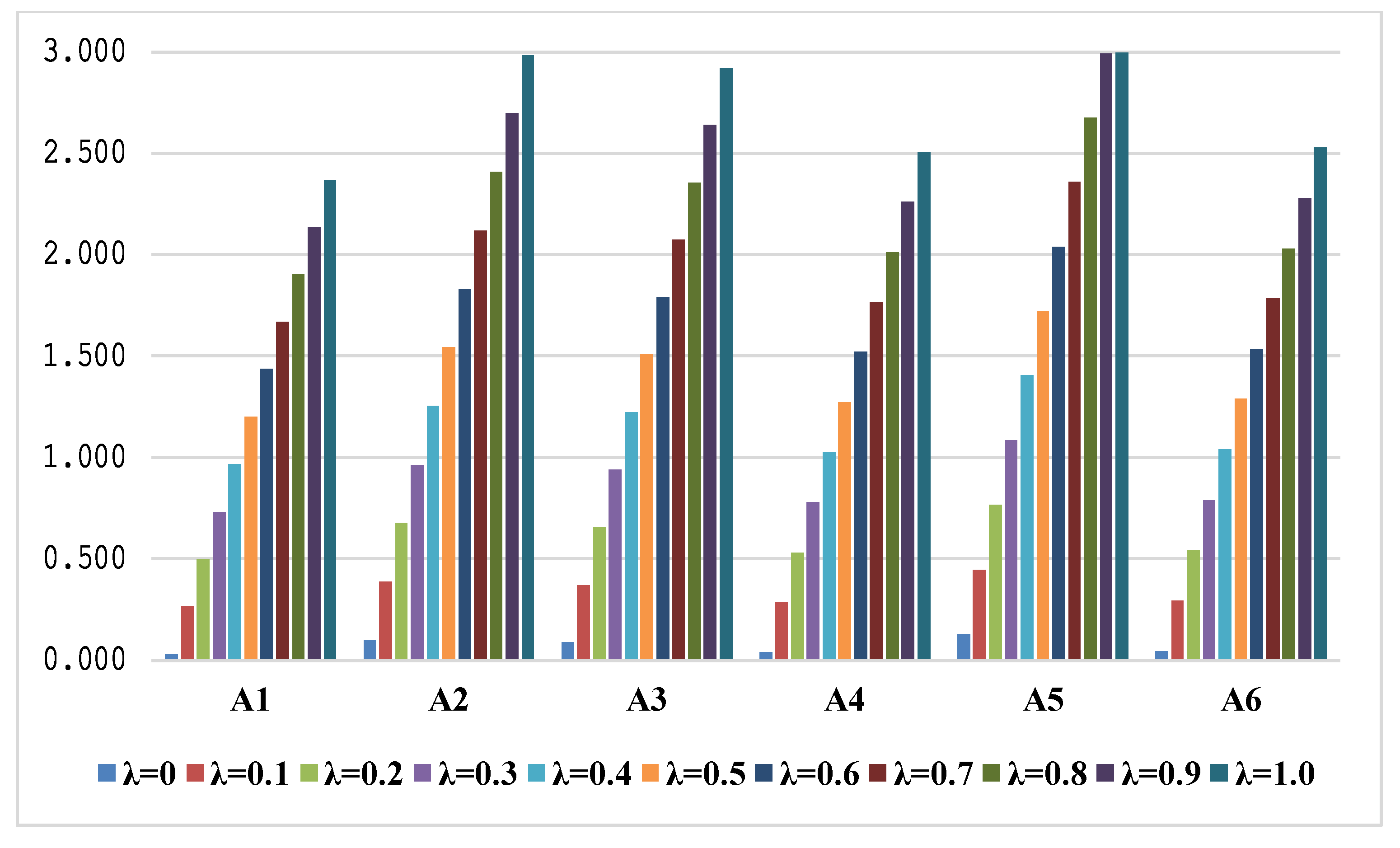
Table 9 and Figure 1 show the relative values of the alternatives depending on the value of the coefficient λ. It can be noted that the values of the coefficient λ do not affect the change in the rank of the alternative, but actually retain their starting rank, as shown in Table 8. As the value of λ increases, the relative values of the alternatives are also increased.

The relative value of the alternative A₁ increases by 0.234 with increasing values of λ, while the second alternative (A₂) increases by 0.289. A slightly smaller increase compared to the previous alternative is in alternative A₃ (by 0.284), while in alternative A₄ it is 0.247. The best alternative is A₅ and it is logical that its value is increased depending on λ at most by 0.319. The last alternative, A₆, is closest to the fourth alternative (A₄) and has an increase of 0.248.

The second part of the sensitivity analysis relates to the application of different MCDM methods in combination with rough numbers that are very recently developed. The model presented in the paper is solved by using the following methods: rough SAW [39], rough EDAS [35], rough MABAC [32], rough VIKOR [47], rough MAIRCA [43] and rough MULTIMOORA [35]. Their results and comparison with the rough WASPAS approach are shown in Figure 2.

Figure 2 shows a comparison of the initial rank obtained by applying a newly developed rough WASPAS approach with other similar approaches to determine the validity of the developed approach. The best alternative does not change its ranking, it is always ranked the first, regardless of the applied approach. The alternative A₁ is at the last place in the application of all other methods, except when using rough VIKOR when it is in fourth place. An alternative A₂ is in the second position, in all cases, except in the rough EDAS method, when it is in third place. The alternative number three (A₃) also retains its position in the ranks of the other approaches, except in the rough EDAS approach where a rotation of position appears, so the alternative three occupy the second place. The alternative four (A₄) is three times in fifth place, three times in fourth place and at the last, sixth place, when the rough VIKOR method is applied. Alternative six (A₆) occupies the fourth place at rough SAW and rough MULTIMOORA, while in the other methods it is in fifth position. Based on all the results and rankings in all the approaches, stability in the rank correlation can be seen, but in order to validate them Spearman’s coefficient of correlation (rk) for statistical comparison of ranks was applied. A comparison of the ranks was done through a comparison of all 7 hybrid models, as shown in

Table 10. Statistical comparison of ranks for tested models.

Methods	RWASPAS	RSAW	REDAS	RMABAC	RVIKOR	RMAIRCA	RMULTI-MOORA	Average
RWASPAS	1.000	1.000	0.886	0.943	0.829	0.943	1.000	0.943
RSAW	-	1.000	0.886	0.943	0.829	0.943	1.000	0.933
REDAS	-	-	1.000	0.943	0.714	0.943	0.886	0.897
RMABAC	-	-	-	1.000	0.771	1.000	0.943	0.929
RVIKOR	-	-	-	-	1.000	0.771	0.829	0.867
RMAIRCA	-	-	-	-	-	1.000	0.943	0.971
RMULTI-MOORA	-	-	-	-	-	-	1.000	1.000
Overall average								0.934

.

From Table 10 it is possible to notice that there is a strong correlation of the ranges between the considered models, since the total mean value of the correlation coefficient is rk = 0.934. The smallest correlation of ranks is when comparing the Rough EDAS approach with Rough VIKOR, Rough MABAC with Rough VIKOR, and Rough VIKOR with Rough MAIRCA, where the values 0.714, 0.717 and 0.717 were obtained, respectively. These are unique situations where rk < 0.80. In other ranking comparison situations, the coefficient of correlation ranges from 0.829 to1.00. Rough WASPAS and Rough SAW have identical ranks, and the correlation coefficient is equal to 1.00, so these two approaches have rk = 0.829 in comparison with the Rough VIKOR approach. The same correlation coefficient value has Rough VIKOR with Rough MULTIMOORA, while the values of 0.886 have Rough WASPAS and Rough SAW with Rough MABAC, and Rough EDAS with Rough MULTIMOORA. The value of the correlation coefficient of 0.943 has Rough WASPAS, Rough SAW and Rough EDAS with Rough MABAC and with Rough MAIRCA, Rough MABAC and Rough MAIRCA with Rough MULTIMOORA. A complete correlation of ranks, besides already mentioned Rough WASPAS and Rough SAW interdependence, the latter methods have with Rough MULTIMOORA, and Rough MABAC with Rough MAIRCA. It can be concluded that there is an extremely strong correlation of ranks and that the ranks obtained by the proposed new approach are confirmed and credible.

6. Conclusions

The developed approach presented in this research refers to the integration of the rough AHP and rough WASPAS methods, where rough AHP is used to calculate the weight values of the criteria, and rough WASPAS is applied for the evaluation and ranking of suppliers. The model is verified through the process of selecting suppliers in the company for the production of PVC furniture based on nine criteria. The results obtained using the rough WASPAS approach show that the fifth alternative is the best solution, in both parts of the sensitivity analysis, that involves changing the value of the coefficient λ and solving the set model with various approaches developed in recent times. Analysis of the results obtained through the calculation of Spearman’s correlation coefficient found that the rough WASPAS approach is in complete correlation with the ranks of other approaches.

Through the research carried out in this paper, two contributions can be distinguished, and one of them is the development of a new rough AHP–rough WASPAS approach which provides an objective aggregation of expert decisions with full observance of inaccuracies and subjectivity that prevails in group decision making. The development of a new approach contributes to the improvement of literature that considers the theoretical and practical application of MCDM methods. The approach that has been developed allows evaluation of alternatives, regardless of imprecision and lack of quantitative information in decision-making. Another contribution of this paper is to improve the methodology of evaluation and selection of suppliers in the production of PVC furniture through a new approach in the treatment of inaccuracies, because the application of this or a similar approach in the selection of suppliers in the field of PVC furniture production has not been identified in the literature. Applying the developed approach, it is possible in a very simple way to solve the problem of MCDM and perform an evaluation and selection of suppliers that has a significant impact on the efficiency of the complete supply chain. The approach developed, besides the considered problem, can also be used for decision making in other areas. Its flexibility is reflected in the fact that verification can be carried out by the integration of any of the multi-criteria decision-making methods for determining the weight values of the criteria. Future research relates to the use of rough numbers in integration with other methods and an attempt to develop a new method in this area.

References

- Petrovic, D.; Xie, Y.; Burnham, K.; Petrovic, R. Coordinated control of distribution supply chains in the presence of fuzzy customer demand. Eur. J. Oper. Res. 2008, 185, 146–158. [Google Scholar] [CrossRef]
- Monczka, R.M.; Handfield, R.B.; Giunipero, L.C.; Patterson, J.L. Purchasing and and Supply Chain Management; Cengage Learning: Boston, MA, USA, 2015; ISBN 978-1-285-86968-1. [Google Scholar]
- Zhong, L.; Yao, L. An ELECTRE I-based multi-criteria group decision making method with interval type-2 fuzzy numbers and its application to supplier selection. Appl. Soft Comput. 2017, 57, 556–576. [Google Scholar] [CrossRef]
- Bai, C.; Sarkis, J. Evaluating supplier development programs with a grey based rough set methodology. Expert Syst. Appl. 2011, 38, 13505–13517. [Google Scholar] [CrossRef]
- Zavadskas, E.K.; Turskis, Z.; Antucheviciene, J.; Zakarevicius, A. Optimization of weighted aggregated sum product assessment. Elektron. Elektrotech. 2012, 122, 3–6. [Google Scholar] [CrossRef]
- Ighravwe, D.E.; Oke, S.A. A fuzzy-grey-weighted aggregate sum product assessment methodical approach for multi-criteria analysis of maintenance performance systems. Int. J. Syst. Assur. Eng. Manag. 2017, 8, 961–973. [Google Scholar] [CrossRef]
- Mathew, M.; Sahu, S.; Upadhyay, A.K. Effect of normalization techniques in robot selection using weighted aggregated sum product assessment. Int. J. Innov. Res. Adv. Stud. 2017, 4, 59–63. [Google Scholar]
- Bagočius, V.; Zavadskas, E.K.; Turskis, Z. Multi-person selection of the best wind turbine based on the multi-criteria integrated additive-multiplicative utility function. J. Civ. Eng. Manag. 2014, 20, 590–599. [Google Scholar] [CrossRef]
- Yazdani, M. New approach to select materials using MADM tools. Int. J. Bus. Syst. Res. 2018, 12, 25–42. [Google Scholar] [CrossRef]
- Hashemkhani Zolfani, S.; Aghdaie, M.H.; Derakhti, A.; Zavadskas, E.K.; Varzandeh, M.H.M. Decision making on business issues with foresight perspective; an application of new hybrid MCDM model in shopping mall locating. Expert Syst. Appl. 2013, 40, 7111–7121. [Google Scholar] [CrossRef]
- Zavadskas, E.K.; Kalibatas, D.; Kalibatiene, D. A multi-attribute assessment using WASPAS for choosing an optimal indoor environment. Arch. Civ. Mech. Eng. 2016, 16, 76–85. [Google Scholar] [CrossRef]
- Suresh, R.K.; Krishnaiah, G.; Venkataramaiah, P. An experimental investigation towards multi objective optimization during hard turning of tool steel using a novel MCDM technique. Int. J. Appl. Eng. Res. 2017, 12, 1899–1907. [Google Scholar]
- Džiugaitė-Tumėnienė, R.; Lapinskienė, V. The multicriteria assessment model for an energy supply system of a low energy house. Eng. Struct. Technol. 2014, 6, 33–41. [Google Scholar] [CrossRef]
- Turskis, Z.; Daniūnas, A.; Zavadskas, E.K.; Medzvieckas, J. Multicriteria evaluation of building foundation alternatives. Comput. Aided Civ. Infrastruct. Eng. 2016, 31, 717–729. [Google Scholar] [CrossRef]
- Emovon, I. A Model for determining appropriate speed breaker mechanism for power generation. J. Appl. Sci. Process Eng. 2018, 5, 256–265. [Google Scholar]
- Madić, M.; Gecevska, V.; Radovanović, M.; Petković, D. Multicriteria economic analysis of machining processes using the WASPAS method. J. Prod. Eng. 2014, 17, 1–6. [Google Scholar]
- Turskis, Z.; Zavadskas, E.K.; Antucheviciene, J.; Kosareva, N. A hybrid model based on fuzzy AHP and fuzzy WASPAS for construction site selection. Int. J. Comput. Commun. Control 2015, 10, 113–128. [Google Scholar] [CrossRef]
- Madic, M.; Antucheviciene, J.; Radovanovic, M.; Petkovic, D. Determination of manufacturing process conditions by using MCDM methods: Application in laser cutting. Eng. Econ. 2016, 27, 144–150. [Google Scholar] [CrossRef]
- Vafaeipour, M.; Zolfani, S.H.; Varzandeh, M.H.M.; Derakhti, A.; Eshkalag, M.K. Assessment of regions priority for implementation of solar projects in Iran: New application of a hybrid multi-criteria decision making approach. Energy Convers. Manag. 2014, 86, 653–663. [Google Scholar] [CrossRef]
- Ghorshi Nezhad, M.R.; Zolfani, S.H.; Moztarzadeh, F.; Zavadskas, E.K.; Bahrami, M. Planning the priority of high tech industries based on SWARA-WASPAS methodology: The case of the nanotechnology industry in Iran. Econ. Res.-Ekon. Istraz. 2015, 28, 1111–1137. [Google Scholar] [CrossRef]
- Yazdani, M.; Hashemkhani Zolfani, S.; Zavadskas, E.K. New integration of MCDM methods and QFD in the selection of green suppliers. J. Bus. Econ. Manag. 2016, 17, 1097–1113. [Google Scholar] [CrossRef]
- Urosevic, S.; Karabasevic, D.; Stanujkic, D.; Maksimovic, M. An approach to personnel selection in the tourism industry based on the SWARA and the WASPAS methods. Econ. Comput. Econ. Cybern. Stud. Res. 2017, 51, 75–88. [Google Scholar]
- Mardani, A.; Nilashi, M.; Zakuan, N.; Loganathan, N.; Soheilirad, S.; Saman, M.Z.M.; Ibrahim, O. A systematic review and meta-Analysis of SWARA and WASPAS methods: Theory and applications with recent fuzzy developments. Appl. Soft Comput. 2017, 57, 265–292. [Google Scholar] [CrossRef]
- Zavadskas, E.K.; Turskis, Z.; Antucheviciene, J. Selecting a contractor by using a novel method for multiple attribute analysis: Weighted Aggregated Sum Product Assessment with grey values (WASPAS-G). Stud. Inform. Control 2015, 24, 141–150. [Google Scholar] [CrossRef]
- Keshavarz Ghorabaee, M.; Zavadskas, E.K.; Amiri, M.; Esmaeili, A. Multi-criteria evaluation of green suppliers using an extended WASPAS method with interval type-2 fuzzy sets. J. Clean. Prod. 2016, 137, 213–229. [Google Scholar] [CrossRef]
- Keshavarz Ghorabaee, M.; Amiri, M.; Zavadskas, E.K.; Antuchevičienė, J. Assessment of third-party logistics providers using a CRITIC–WASPAS approach with interval type-2 fuzzy sets. Transport 2017, 32, 66–78. [Google Scholar] [CrossRef]
- Zavadskas, E.K.; Baušys, R.; Stanujkic, D.; Magdalinovic-Kalinovic, M. Selection of lead-zinc flotation circuit design by applying WASPAS method with single-valued neutrosophic set. Acta Montan. Slov. 2016, 21, 85–92. [Google Scholar]
- Baušys, R.; Juodagalvienė, B. Garage location selection for residential house by WASPAS-SVNS method. J. Civ. Eng. Manag. 2017, 23, 421–429. [Google Scholar] [CrossRef]
- Zavadskas, E.K.; Antucheviciene, J.; Hajiagha, S.H.R.; Hashemi, S.S. Extension of weighted aggregated sum product assessment with interval-valued intuitionistic fuzzy numbers (WASPAS-IVIF). Appl. Soft Comput. 2014, 24, 1013–1021. [Google Scholar] [CrossRef]
- Nie, R.X.; Wang, J.Q.; Zhang, H.Y. Solving solar-wind power station location problem using an extended weighted aggregated sum product assessment (WASPAS) technique with interval neutrosophic sets. Symmetry 2017, 9, 106. [Google Scholar] [CrossRef]
- Song, W.; Ming, X.; Wu, Z.; Zhu, B. A rough TOPSIS approach for failure mode and effects analysis in uncertain environments. Qual. Reliab. Eng. Int. 2014, 30, 473–486. [Google Scholar] [CrossRef]
- Roy, J.; Chatterjee, K.; Bandhopadhyay, A.; Kar, S. Evaluation and selection of Medical Tourism sites: A rough AHP based MABAC approach. arXiv, 2016; arXiv:1606.08962. [Google Scholar]
- Pamučar, D.; Stević, Ž.; Zavadskas, E.K. Integration of interval rough AHP and interval rough MABAC methods for evaluating university web pages. Appl. Soft Comput. 2018, 67, 141–163. [Google Scholar] [CrossRef]
- Song, W.; Ming, X.; Wu, Z. An integrated rough number-based approach to design concept evaluation under subjective environments. J. Eng. Des. 2013, 24, 320–341. [Google Scholar] [CrossRef]
- Stević, Ž.; Pamučar, D.; Vasiljević, M.; Stojić, G.; Korica, S. Novel integrated multi-criteria model for supplier selection: Case study construction company. Symmetry 2017, 9, 279. [Google Scholar] [CrossRef]
- Cao, J.; Song, W. Risk assessment of co-creating value with customers: A rough group analytic network process approach. Expert Syst. Appl. 2016, 55, 145–156. [Google Scholar] [CrossRef]
- Vasiljevic, M.; Fazlollahtabar, H.; Stevic, Z.; Veskovic, S. A rough multicriteria approach for evaluation of the supplier criteria in automotive industry. Decis. Mak. Appl. Manag. Eng. 2018, 1, 82–96. [Google Scholar] [CrossRef]
- Karavidic, Z.; Projovic, D. A multi-criteria decision-making (MCDM) model in the security forces operations based on rough sets. Decis. Mak. Appl. Manag. Eng. 2018, 1, 97–120. [Google Scholar] [CrossRef]
- Stević, Ž.; Pamučar, D.; Zavadskas, E.K.; Ćirović, G.; Prentkovskis, O. The selection of wagons for the internal transport of a logistics company: A novel approach based on Rough BWM and Rough SAW Methods. Symmetry 2017, 9, 264. [Google Scholar] [CrossRef]
- Chai, J.; Liu, J.N. A novel believable rough set approach for supplier selection. Expert Syst. Appl. 2014, 41, 92–104. [Google Scholar] [CrossRef]
- Zhai, L.Y.; Khoo, L.P.; Zhong, Z.W. Design concept evaluation in product development using rough sets and grey relation analysis. Expert Syst. Appl. 2009, 36, 7072–7079. [Google Scholar] [CrossRef]
- Khoo, L.P.; Tor, S.B.; Zhai, L.Y. A rough-set based approach for classification and rule induction. Int. J. Adv. Manuf. Technol. 1999, 15, 438–444. [Google Scholar] [CrossRef]
- Pamučar, D.; Mihajlović, M.; Obradović, R.; Atanasković, P. Novel approach to group multi-criteria decision making based on interval rough numbers: Hybrid DEMATEL-ANP-MAIRCA model. Expert Syst. Appl. 2017, 88, 58–80. [Google Scholar] [CrossRef]
- Duntsch, I.; Gediga, G. The rough set engine GROBIAN. In Proceedings of the 15th IMACS World Congress; Sydow, A., Ed.; Berlin Wissenschaft und Technik Verlag: Berlin, Germany, 1997; Volume 4, pp. 613–618. [Google Scholar]
- Khoo, L.-P.; Zhai, L.-Y. A prototype genetic algorithm enhanced rough set-based rule induction system. Comput. Ind. 2001, 46, 95–106. [Google Scholar] [CrossRef]
- Pawlak, Z. Rough sets. Int. J. Comput. Inf. Sci. 1982, 11, 341–356. [Google Scholar] [CrossRef]
- Zhu, G.N.; Hu, J.; Qi, J.; Gu, C.C.; Peng, J.H. An integrated AHP and VIKOR for design concept evaluation based on rough number. Adv. Eng. Inform. 2015, 29, 408–418. [Google Scholar] [CrossRef]
- Pawlak, Z. Rough Sets: Theoretical Aspects of Reasoning about Data; Springer: Berlin, Germany, 1991. [Google Scholar]
- Pawlak, Z. Anatomy of conflicts. Bull. Eur. Assoc. Theor. Comput. Sci. 1993, 50, 234–247. [Google Scholar]
- Stević, Ž. Integrisani Model Vrednovanja Dobavljača u Lancima Snabdevanja. Ph.D. Thesis, Univerzitet u Novom Sadu, Fakultet Tehničkih Nauka, Novi Sad, Serbia, 2018. (In Bosnian). [Google Scholar]
- Zhai, L.Y.; Khoo, L.P.; Zhong, Z.W. A rough set based QFD approach to the management of imprecise design information in product development. Adv. Eng. Inform. 2009, 23, 222–228. [Google Scholar] [CrossRef]
Figure 1.
Results of sensitivity analysis dependent on coefficient λ.
Figure 2.
Results of sensitivity analysis in comparison with other rough methods.