Element-Weighted Neutrosophic Correlation Coefficient and Its Application in Improving CAMShift Tracker in RGBD Video

Abstract

Neutrosophic set (NS) is a new branch of philosophy to deal with the origin, nature, and scope of neutralities. Many kinds of correlation coefficients and similarity measures have been proposed in neutrosophic domain. In this work, by considering that there may exist different contributions for the neutrosophic elements of T (Truth), I (Indeterminacy), and F (Falsity), a method of element-weighted neutrosophic correlation coefficient is proposed, and it is applied for improving the CAMShift tracker in RGBD (RGB-Depth) video. The concept of object seeds is proposed, and it is employed for extracting object region and calculating the depth back-projection. Each candidate seed is represented in the single-valued neutrosophic set (SVNS) domain via three membership functions, T, I, and F. Then the element-weighted neutrosophic correlation coefficient is applied for selecting robust object seeds by fusing three kinds of criteria. Moreover, the proposed correlation coefficient is applied for estimating a robust back-projection by fusing the information in both color and depth domains. Finally, for the scale adaption problem, two alternatives in the neutrosophic domain are proposed, and the corresponding correlation coefficient between the proposed alternative and the ideal one is employed for the identification of the scale. When considering challenging factors like fast motion, blur, illumination variation, deformation, and camera jitter, the experimental results revealed that the improved CAMShift tracker performs well.

1. Introduction

A neutrosophic set (NS) [1] is suitable for dealing with problems with indeterminate information. A neutrosophic set is always characterized independently via three membership functions, T, I, and F. These functions in the universal set X are real standard or nonstandard subsets of [⁻0, 1⁺]. It is difficult to introduce the NS theory into science and engineering areas when considering the non-standard unit interval. The single-valued neutrosophic set (SVNS) [2] was proposed to handle such a problem. The membership functions are restrained to the normal standard real unit interval [0, 1].

Until now, NS has been successfully applied in a lot of fields [3] such as medical diagnosis [4], image segmentation [5,6,7,8,9], skeleton extraction [10], and object tracking [11,12]. Several similarity measurements or multicriteria decision-making methods [13,14,15,16,17,18,19,20] were employed to handle the neutrosophic problems. Decision-making can be regarded as a problem-solving activity terminating in a solution deemed to be satisfactory. It has been applied for residential house garage location selection [18], element and material selection [19], and sustainable market valuation of buildings [20]. For the application of image segmentation, several criteria in the NS domain were usually proposed for calculating a specific neutrosophic image [5,6,7,8,9]. The correlation coefficient between SVNSs [17] was applied for calculating a neutrosophic score-based image [9], and a robust threshold was estimated by employing the OTSU’s method [9]. In [11], two criteria were proposed in both color and depth domain. The information fusion problem was converted into a multicriteria decision-making issue, and the single-valued neutrosophic cross-entropy was employed to tackle this problem [11]. For the neutrosophic theory-based MeanShift tracker [12], by taking the consideration of the background information and appearance changes between frames, two kinds of criteria were considered, the object feature similarity and the background feature similarity. The SVNS correlation coefficient [17] was applied for calculating the weighted histogram, and then the histogram was finally used to enhance the traditional MeanShift tracker. Besides the fields mentioned above, the NS theory was also introduced into clustering algorithms such as c-means [21]. While NS-based correlation coefficients have been widely used for solving some engineering issues, the weights of the three membership functions are always treated equally. However, for the elements of T, I, and F, different contributions should be taken into consideration of the results of decision-making. In this work, a method of element-weighted neutrosophic correlation coefficient is proposed, and we try to utilize it for tracking a visual object in RGBD (RGB-Depth) video.

Visual object tracking is still an open issue [22,23,24], and its robustness still lacks the performance of vision applications like surveillance, traffic monitoring, video indexing, and auto-driving. For a tracking task, challenges like background clutter, fast motion, illumination variation, scale variation, motion blur, and camera jitter may happen during the tracking procedure. Two methods are considered to handle these challenging problems. One is utilizing robust features. The color feature is employed by the MeanShift [25] and CAMShift [26] tracker, due to its robustness when there exist challenges like deformation, blur, and rotation. Both trackers are of high efficiency [27]. However, when the surroundings have a similar color, they may easily drift from the target. To deal with such a problem, Cross-Bin metric [28], scale-invariant feature transform (SIFT) [29], and texture feature [30] were introduced into the mean shift-based tracker, and better performance was achieved. The other way is to train robust models, such as the multiple instance learning [31,32] and compressive sensing [33]-based tracking. Besides the kinds of trackers mentioned above, the local-global tracker (LGT) [34], incremental visual tracker (IVT) [35] and tracking-learning-detection (TLD) [36] also perform well.

Recently, due to the fact that the depth information can provide another dimension for tackling the object tracking problem, some RGBD-based trackers [11,37,38,39] have been proposed. Most algorithms are oriented to specific targets [37,38,39]. A few category-free RGBD trackers have been proposed. An improved CAMShift tracker was proposed by using the neutrosophic decision-making method in [11], but the indeterminate information was only considered in the information fusion phase. As mentioned above, the CAMShift tracker will perform well, with high efficiency, if a discriminative feature can be employed. In this work, based on the CAMShift framework, we focus on tackling the visual tracking problem when challenges like fast motion, blur, illumination variation, deformation, and camera jitter exist, but without serious occlusion. It is difficult to find such a tracker due to the fact that tracking an object without occlusion is still very challenging for both RGB and RGBD trackers. For the CAMShift tracker, calculating a robust back-projection is one of the most important issues for tracking a target. Indeterminate information always exists in the procedure of the CAMShift process. For instance, it exists when estimating the likelihood probability map, as well as localizing the target. In this work, we try to utilize the method of element-weighted neutrosophic correlation coefficient to handling decision-making problems when there is indeterminate information.

This work mainly exhibits four contributions. First, a method of element-weighted neutrosophic correlation coefficient is proposed. Secondly, three criteria are proposed for object seeds selection, and the corresponding membership functions, T, I, and F, are given. Thirdly, the proposed correlation coefficient is applied for estimating a robust back-projection by fusing the information in both color and depth domains. Finally, for the scale adaption problem, two alternatives in the neutrosophic domain are proposed, and the corresponding correlation coefficient between the proposed alternative and the ideal one is employed for the identification of the scale.

The remainder of this paper is organized as follows: in Section 2, the element-weighted neutrosophic correlation coefficient is presented. In Section 3, main steps and basic flow of the improved CAMShift visual tracker is given first, and the details are illustrated in the following subsections. Experimental evaluations and discussions are presented in Section 4, and Section 5 is the conclusions.

2. Element-Weighted Neutrosophic Correlation Coefficient

2.1. Neutrosophic Correlation Coefficient

Let $A=\left\{A_1,A_2,\mathrm{\dots }{A}_m\right\}$ be a set of alternatives and $C=\left\{C_1,C_2,\mathrm{\dots }{C}_n\right\}$ be a set of criteria. We get

$$A_i=\left\{\langle C_j,T_{C_j}(A_i),I_{C_j}(A_i),F_{C_j}(A_i)\rangle |C_j\in C\right\}i=1\dots m,j=1\dots n,$$

(1)

where A_i is an alternative in A, $T_{C_j}(A_i)$ indicates the degree to which the alternative A_i satisfies the criterion C_j; $I_{C_j}(A_i)$ denotes the indeterminacy degree to which the alternative A_i satisfies or does not satisfy the criterion C_j; $F_{C_j}(A_i)$ denotes the degree to which the alternative A_i does not satisfy the criterion C_j, $T_{C_j}(A_i)$, $I_{C_j}(A_i)$, $F_{C_j}(A_i)\in [0,1]$, $1\le T_{C_j}(A_i)+I_{C_j}(A_i)+F_{C_j}(A_i)\le 3$, and A is a single-valued neutrosophic set.

The correlation coefficient under single-valued neutrosophic environment between two alternatives A_i and A_j is defined as [17]:

$$S_{C_k}(A_i,A_j)=\frac{T_{C_k}(A_i)T_{C_k}(A_j)+I_{C_k}(A_i)I_{C_k}(A_j)+F_{C_k}(A_i)F_{C_k}(A_j)}{\sqrt{T_{C_k}{}^2(A_i)+I_{C_k}{}^2(A_i)+F_{C_k}{}^2(A_i)}\sqrt{T_{C_k}{}^2(A_j)+I_{C_k}{}^2(A_j)+F_{C_k}{}^2(A_j)}}.$$

(2)

Considering the contribution of each criterion, the weighted correlation coefficient between A_i and A_j is defined by

$$W(A_i,A_j)={\displaystyle \sum _{k=1}^n{w}_k\frac{T_{C_k}(A_i)T_{C_k}(A_j)+I_{C_k}(A_i)I_{C_k}(A_j)+F_{C_k}(A_i)F_{C_k}(A_j)}{\sqrt{T_{C_k}{}^2(A_i)+I_{C_k}{}^2(A_i)+F_{C_k}{}^2(A_i)}\sqrt{T_{C_k}{}^2(A_j)+I_{C_k}{}^2(A_j)+F_{C_k}{}^2(A_j)}}},$$

(3)

where w_k $\in$ [0,1] is the weight of each criterion C_k and ${\displaystyle {\sum }_{j=1}^n{w}_j}=1$.

Assume A* is the ideal alternative, $A^{\ast }=\left\{\langle C_j,T_{C_j}(A^{\ast }),I_{C_j}(A^{\ast }),F_{C_j}(A^{\ast })\rangle |C_j\in C\right\}$. Then the weighted correlation coefficient between any alternative A_i and the ideal alternative A* can be calculated by

$$W(A_i,A^{\ast })={\displaystyle \sum _{k=1}^n{w}_k\frac{T_{C_k}(A_i)T_{C_k}(A^{\ast })+I_{C_k}(A_i)I_{C_k}(A^{\ast })+F_{C_k}(A_i)F_{C_k}(A^{\ast })}{\sqrt{T_{C_k}{}^2(A_i)+I_{C_k}{}^2(A_i)+F_{C_k}{}^2(A_i)}\sqrt{T_{C_k}{}^2(A^{\ast })+I_{C_k}{}^2(A^{\ast })+F_{C_k}{}^2(A^{\ast })}}}.$$

(4)

2.2. Element-Weighted Neutrosophic Correlation Coefficient

As seen in Equation (3), only the contribution of each criterion is considered. However, in some engineering applications, it is better to provide specific weights for the T, I, and F elements for an alternative A_i when considering the criteria C_j. The element-weighted correlation coefficient between A_i and A_j is defined by

$$S_e(A_i,A_j)=\frac{\alpha T_{C_k}(A_i)T_{C_k}(A_j)+\beta I_{C_k}(A_i)I_{C_k}(A_j)+\gamma F_{C_k}(A_i)F_{C_k}(A_j)}{\sqrt{\alpha T_{C_k}{}^2(A_i)+\beta I_{C_k}{}^2(A_i)+\gamma F_{C_k}{}^2(A_i)}\sqrt{\alpha T_{C_k}{}^2(A_j)+\beta I_{C_k}{}^2(A_j)+\gamma F_{C_k}{}^2(A_j)}},$$

(5)

where α, β, γ $\in$ [0,1], α + β + γ = 1. Then $S_e(A_i,A_j)$ is actually the cosine value between the vector $(\sqrt{\alpha }{T}_{C_k}(A_i),\sqrt{\beta }{I}_{C_k}(A_i),\sqrt{\gamma }{F}_{C_k}(A_i))$ and $(\sqrt{\alpha }{T}_{C_k}(A_j),\sqrt{\beta }{I}_{C_k}(A_j),\sqrt{\gamma }{F}_{C_k}(A_j))$. Hence, it is easy to find that Se satisfies the following properties:

(SP1) $0\le S_e(A_i,A_j)\le 1$;

(SP2) $S_e(A_i,A_j)=S_e(A_j,A_i)$;

(SP3) $S_e(A_i,A_j)=1if{A}_i=A_j$;

Then the element-criterion-weighted correlation coefficient between A_i and the ideal alternative A* is defined as

$$W{S}_e(A_i,A^{\ast })={\displaystyle \sum _{k=1}^n{w}_k\frac{\alpha T_{C_k}(A_i)T_{C_k}(A^{\ast })+\beta I_{C_k}(A_i)I_{C_k}(A^{\ast })+\gamma F_{C_k}(A_i)F_{C_k}(A^{\ast })}{\sqrt{\alpha T_{C_k}{}^2(A_i)+\beta I_{C_k}{}^2(A_i)+\gamma F_{C_k}{}^2(A_i)}\sqrt{\alpha T_{C_k}{}^2(A^{\ast })+\beta I_{C_k}{}^2(A^{\ast })+\gamma F_{C_k}{}^2(A^{\ast })}}}$$

(6)

3. Improved CAMShift Visual Tracker Based on the Neutrosophic Theory

The algorithmic details of the proposed tracker are presented in this section.

A rectangle bounding box [22,23] is always employed for the representation of the target location when dealing with the visual tracking problem. For a visual tracker, the critical task is to estimate the corresponding bounding box in each frame.

Algorithm 1 illustrates the basic flow of the proposed algorithm, as seen in

Table 1. Basic flow of the NeutRGBDs tracker.

Algorithm 1 NeutRGBDs
Initialization
Input: 1st video frame in the RGBD domain
(1) Select an object on the image plane
(2) Extract object seeds using both color and depth information
(3) Extract object region using object seeds and the information of the depth segmentation
(4) Calculate the corresponding color and depth histograms as target model
Tracking
Input: (t+1)-th video frame in the RGBD domain
(1) Calculate back-projections in both color (Pc) and depth domain (PD)
(2) Calculate fused back-projection (P) using neutrosophic theory
(3) Calculate the bounding box of the target in the CAMShift framework
(4) Extract object region and update object model and seeds
(5) Modify the scale of the bounding box in neutrosophic domain
Output: Tracking location

. Details of each main step are given in the following subsections.

3.1. Selecting Object Seeds

Assuming the tracker can calculate an adequate bounding box, and R is the extracted object region, then it is reasonable that we assume pixels located in R and the bounding box with smaller depth value are more likely to be a part of the target.

To select robust object seeds, the pixels located in R and the bounding box are first sorted by the descending order of the depth value. Then several pixels are selected as the candidate object seeds set S by sampling the sorted pixels with a fixed sampling space. Considering there may exists background regions in the corresponding area, only the top 50 percent pixels in the sorted pixel set are sampled.

For the proposition of depth value is a critical criterion for judging the object seed, T_D, I_D, and F_D represent the probabilities when a proposition is true, indeterminate and false degrees, respectively. Then we can give the definitions:

$$T_D=\frac{r_{\max }-r_{si}}{r_{\max }}$$

(7)

$$I_D=\mathrm{var}(D(RO{I}_{si}))$$

(8)

$$F_D=1-T_D,$$

(9)

where r_max is the lowest rank in S, and r_si is the rank of the i-th candidate seed S_i; ROI_si is a set of pixels that is located in the square area centered at S_i, and the length of the sides of the square should be set to an odd value; D(ROI_si) is the depth value set corresponding to ROI_si, and var(x) is the standard variance function.

As there may be other objects with a similar depth to the tracked target, the color similarity criterion is considered in this work to conquer such a problem. The corresponding three membership functions T_C, I_C and F_C are defined as follows:

$$T_C=P_c(S_i)$$

(10)

$$I_C=\mathrm{var}(P_c(RO{I}_{si}))$$

(11)

$$F_C=1-T_C,$$

(12)

where P_c is the back-projection calculated in color domain; P_c(S_i) is the value of the back-projection located at S_i. P_c(ROI_si) is the value set corresponding to ROI_si in P_c.

Besides the consideration of the depth and color feature separately, the fused color-depth information is also taken into consideration. The corresponding three membership functions T_DC, I_DC and F_DC for the fused color-depth criterion are defined as follows:

$$T_{DC}=P(S_i)$$

(13)

$$I_{DC}=\mathrm{var}(P(RO{I}_{si}))$$

(14)

$$F_{DC}=1-T_{DC},$$

(15)

where P is the fused back-projection; P(S_i) is the value of the back-projection located at S_i; P(ROI_si) is the value set corresponding to ROI_si in P.

By substituting the corresponding T, I, and F under the proposed three criteria into Equation (6), the probability of the reliability for the seed S_i can be calculated by

$$\begin{array}{lll}p{r}_{si}& =& w_{D}p{r}_{Dsi}+w_{C}p{r}_{Csi}+w_{DC}p{r}_{DCsi}\\ & =& w_D\frac{\alpha T_D{T}_D(A^{\ast })+\beta I_D{I}_D(A^{\ast })+\gamma F_D{F}_D(A^{\ast })}{\sqrt{\alpha T_D{}^2+\beta I_D{}^2+\gamma F_D{}^2}\sqrt{\alpha T_D{}^2(A^{\ast })+\beta I_D{}^2(A^{\ast })+\gamma F_D{}^2(A^{\ast })}}\\ & & +w_C\frac{\alpha T_C{T}_C(A^{\ast })+\beta I_C{I}_C(A^{\ast })+\gamma F_C{F}_C(A^{\ast })}{\sqrt{\alpha T_C{}^2+\beta I_C{}^2+\gamma F_C{}^2}\sqrt{\alpha T_C{}^2(A^{\ast })+\beta I_C{}^2(A^{\ast })+\gamma F_C{}^2(A^{\ast })}}\\ & & +w_{DC}\frac{\alpha T_{DC}{T}_{DC}(A^{\ast })+\beta I_{DC}{I}_{DC}(A^{\ast })+\gamma F_{DC}{F}_{DC}(A^{\ast })}{\sqrt{\alpha T_{DC}{}^2+\beta I_{DC}{}^2+\gamma F_{DC}{}^2}\sqrt{\alpha T_{DC}{}^2(A^{\ast })+\beta I_{DC}{}^2(A^{\ast })+\gamma F_{DC}{}^2(A^{\ast })}}\end{array},$$

(16)

where w_D, w_C, w_DC $\in$ [0,1] are the corresponding weights of criteria and w_D + w_C + w_DC = 1. Assuming the ideal alternative under all the three criteria is the same as $A^{\ast }=\langle 1,0,0\rangle$, then Equation (16) can be simplified to

$$p{r}_{si}=\sqrt{\alpha }\left(\begin{array}{l}{w}_D\frac{T_D}{\sqrt{\alpha T_D{}^2+\beta I_D{}^2+\gamma F_D{}^2}}+w_C\frac{T_C}{\sqrt{\alpha T_C{}^2+\beta I_C{}^2+\gamma F_C{}^2}}\\ +w_{DC}\frac{T_{DC}}{\sqrt{\alpha T_{DC}{}^2+\beta I_{DC}{}^2+\gamma F_{DC}{}^2}}\end{array}\right).$$

(17)

After calculating all the probability of the reliability for the seed in S, the first N seeds sorted by pr_si are selected as object seeds set OS.

3.2. Extracting Object

The critical task for extracting object is to determine the extracted object region R.

For each frame, the image is segmented into regions in the depth domain. In this work, the fast depth segmentation method [40] is employed for segmentation. Suppose there exist M regions in the t-th frame, C_i represents the i-th region, and DC_i is the depth value at the location of the centroid of C_i.

Suppose OS_i is the i-th object seed in the previous frame and B is the pixel set located in the area of the bounding box calculated by the tracker in the current frame. The extracted region R is defined as:

$$R=\left\{\cup \left(C_k\cap B\right)|\min \left(\left|D{C}_k-DO{S}_i\right|\right)<T,i=1,2,\mathrm{\dots }N\right\},$$

(18)

where DOS_i is the depth value of OS_i; T is a threshold value; $\cup$ and $\cap$ corresponds to the set operation. All the regions C_k belonging to R constructs the candidate object region RC.

3.3. Calculating the Fused Back-Projection

Back-projection is a probability distribution map with the same size as the input image. Each pixel value of the back-projection demonstrates the likelihood of the corresponding pixel belonging to the tracked object. Considering that using the discriminative feature is one of the most important factors for the visual tracker, both the color and depth information are employed for calculating the fused back-projection.

In [11], two criteria are proposed in both feature domain. For the near region similarity criterion, the corresponding neutrosophic elements are defined as follows:

$$T_{Cn}={\displaystyle \sum _{u=1}^{m^c}\sqrt[]{{\widehat{q}}_u^c{\widehat{p}}_u^c}}$$

(19)

$$I_{Cn}={\displaystyle \sum _{u=1}^{m^c}\sqrt[]{{\widehat{q}}_u^c{\widehat{p}}_u^c{}^{\prime }}}$$

(20)

$$F_{Cn}=1-T_{Cn},$$

(21)

where ${\widehat{q}}_u^c$ is the u-th bin of the feature vector for the target in the color domain, it is firstly calculated in the first frame by

$${\widehat{q}}_u^c=C{\displaystyle \sum _{i=1}^n\delta \left[b^c(x_i)-u\right]},$$

(22)

where ${\left\{x_i\right\}}_i{}_{=1\dots n}$ are the pixels located in the extracted object region R; b^c is the transformation function in color domain, and the function b^c: $R^2\to \left\{1\dots m^c\right\}$ associates to the pixel at location x_i the index b(x_i) of its bin in the quantized feature space; δ is the Kronecker delta function; C is the normalization constant derived by imposing the condition ${\displaystyle {\sum }_{u=1}^{m^c}{\widehat{q}}_u^c}=1$; ${\widehat{p}}_u^c$ is the u-th bin of the feature vector corresponds to the extracted object region R in the current frame, and ${\widehat{p}}_u^c{}^{\prime }$ corresponds to the feature vector in the annular region near the target, as defined in [11].

Similarly, for the near region similarity criterion, the corresponding neutrosophic elements in the depth domain can be computed by

$$T_{Dn}={\displaystyle \sum _{u=1}^{m^d}\sqrt[]{{\widehat{q}}_u^d{\widehat{p}}_u^d}},I_{Dn}={\displaystyle \sum _{u=1}^{m^d}\sqrt[]{{\widehat{q}}_u^d{\widehat{p}}_u^d{}^{\prime }}}, F_{Dn}=1-T_{Dn},$$

(23)

where ${\widehat{q}}_u^d$, ${\widehat{p}}_u^d$ and ${\widehat{p}}_u^d{}^{\prime }$ are the corresponding feature vector in the depth domain, similar to the calculation of ${\widehat{q}}_u^c$, ${\widehat{p}}_u^c$ and ${\widehat{p}}_u^c{}^{\prime }$.

By applying the far region similarity criterion [11], the related functions are presented as follows:

$$\begin{array}{l}{T}_{Cf}={\displaystyle \sum _{u=1}^{m^c}\sqrt[]{{\widehat{q}}_u^c{\widehat{p}}_u^c}},I_{Cf}={\displaystyle \sum _{u=1}^{m^c}\sqrt[]{{\widehat{q}}_u^c{\widehat{p}}_u^c{}^{{\prime }^{\prime }}}},F_{Cf}=1-T_{Cf}\\ T_{Df}={\displaystyle \sum _{u=1}^{m^d}\sqrt[]{{\widehat{q}}_u^d{\widehat{p}}_u^d}},I_{Df}={\displaystyle \sum _{u=1}^{m^d}\sqrt[]{{\widehat{q}}_u^d{\widehat{p}}_u^d{}^{{\prime }^{\prime }}}},F_{Df}=1-T_{Df}\end{array},$$

(24)

where T_Cf, I_Cf, and F_Cf correspond to the color domain; T_Df, I_Df and F_Df are the functions in the depth domain. As defined in [11], ${\widehat{p}}_u^c{}^{{\prime }^{\prime }}$ and ${\widehat{p}}_u^d{}^{{\prime }^{\prime }}$ are the feature vectors in the annular region far from the target in the color and depth domain, respectively.

As discussed in [11], the back-projection in the color domain is defined as

$$P_c(x)={\widehat{q}}_{b^c(x)}^c,$$

(25)

where b^c is the transformation function, as defined in Equation (22), and x is the pixel coordinate on the image plane.

By using the assumption that the tracked target is with a relative low speed, the back-projection corresponding to the depth domain is defined as [11]:

$$P_D(x)=\frac{1}{2}erfc(4\frac{d(x,S)}{MAXD}-2),x\in 2B_{pre},$$

(26)

where d (x, S) is the minimal depth distance between the pixel x and the previous seed set S; MAXD is the maximum depth displacement of the target between adjacent frames; 2B_pre is the pixel set that is covered by a bounding box of twice the size of the previous object location, but with the same center.

By considering the robustness of P_C and P_D, the fused back-projection P can be calculated as

$$P(x)=rc\times P_C{}^{\prime }(x)+(1-rc)\times P_D{}^{\prime }(x),$$

(27)

where rc is calculated by

$$rc=\frac{n{s}_C}{n{s}_C+n{s}_D},$$

(28)

where $n{s}_C$ is the element-weighted correlation coefficient in the color domain. The ideal alternative under the near or far region similarity criterion is the same as $A^{\ast }=\langle 1,0,0\rangle$. Then ns_C is defined as

$$n{s}_C=\sqrt{\alpha }\left(w_{Cn}\frac{T_{Cn}}{\sqrt{\alpha T_{Cn}{}^2+\beta I_{Cn}{}^2+\gamma F_{Cn}{}^2}}+w_{Cf}\frac{T_{Cf}}{\sqrt{\alpha T_{Cf}{}^2+\beta I_{Cf}{}^2+\gamma F_{Cf}{}^2}}\right),$$

(29)

where w_Cn, w_Cf ∈ [0,1] are the corresponding weights of criteria and w_Cn + w_Cf = 1. Similarly, the element-weighted correlation coefficient in the depth domain is defined as

$$n{s}_D=\sqrt{\alpha }\left(w_{Dn}\frac{T_{Dn}}{\sqrt{\alpha T_{Dn}{}^2+\beta I_{Dn}{}^2+\gamma F_{Dn}{}^2}}+w_{Df}\frac{T_{Df}}{\sqrt{\alpha T_{Df}{}^2+\beta I_{Df}{}^2+\gamma F_{Df}{}^2}}\right),$$

(30)

where w_Dn, w_Df ∈ [0,1] are the corresponding weights of criteria and w_Dn + w_Df = 1. For $P_C{}^{\prime }$ and $P_D{}^{\prime }$ defined in Equation (27), they are computed by

$$P_C{}^{\prime }(x)=\{\begin{array}{c}{P}_C(x)if{P}_D(x)>T_D\hfill \\ 0else\hfill \end{array}$$

(31)

$$P_D{}^{\prime }(x)=\{\begin{array}{c}{P}_D(x)if{P}_C(x)>T_C\hfill \\ 0else\hfill \end{array},$$

(32)

where T_D, T_C $\in$ [0,1] are the threshold for filtering the noise in the color or depth back-projection. As seen in Equation (31), the information in P_D is employed for enhancing the color back-projection P_C, and vice versa for Equation (32).

3.4. Scale Adaption

In this work, the bounding box of the tracked object is firstly decided by the traditional CAMShfit algorithm [26]. For each frame, the bounding box B_pre in the previous frame is employed as the start location of the mean shift process. The current tracking location can be calculated by

$$x=\frac{M_{10}}{M_{00}},y=\frac{M_{01}}{M_{00}},$$

(33)

where $M_{10}={\displaystyle {\sum }_{x\in B}xP(x)}$, $M_{01}={\displaystyle {\sum }_{x\in B}yP(x)}$, and $M_{00}={\displaystyle {\sum }_{x\in B}P(x)}$. Then, the size of the bounding box is $s=2\sqrt{M_{00}/256}$. For convenience, this bounding box is called the initial bounding box bellow.

Getting the adequate scale of the bounding box is very important. If the scale cannot fit the object for a few frames, the tracker may finally drift from the target. Considering the size of the initial bounding box may be disturbed by the imprecision of the back-projection, a method in the neutrosophic domain is introduced into the scale identification process.

In this work, the color likelihood probability between the candidate object area and the object area is employed as the truth membership. The color likelihood probability between the candidate object area and the background area is employed as the indetermination membership. For the reducing scale alternative, the truth, indetermination, false membership functions are defined as

$$T_{rs}={\displaystyle \sum _{u=1}^{m^c}\sqrt[]{{\widehat{q}}_u^c{\widehat{p}}_{rsu}^c}}$$

(34)

$$I_{rs}={\displaystyle \sum _{u=1}^{m^c}\sqrt[]{{\widehat{p}}_{rsu}^c{\widehat{b}}_{rsu}^c}}$$

(35)

$$F_{rs}=1-T_{rs},$$

(36)

where ${\widehat{p}}_{rsu}^c$ is the u-th bin of the feature vector in the initial bounding box with a reduced scale; ${\widehat{b}}_{rsu}^c$ corresponds to the feature vector in the annular region nearby the scale-reduced bounding box. It must be emphasized that all the pixels taken into consideration must located in the candidate object region RC in the current frame. By substituting Equations (34)–(36) into the Equation (6) with the assumption that the idea alternative $A^{\ast }=\langle 1,0,0\rangle$, the probability for reducing scale is defined as

$$w_{rs}=\frac{\sqrt{\alpha }{T}_{rs}}{\sqrt{\alpha T_{rs}{}^2+\beta I_{rs}{}^2+\gamma F_{rs}{}^2}}.$$

(37)

Similarly, for the expanding scale alternative, the truth, indetermination, and false membership functions are defined as

$$T_{exs}={\displaystyle \sum _{u=1}^{m^c}\sqrt[]{{\widehat{q}}_u^c{\widehat{p}}_{exsu}^c}}$$

(38)

$$I_{exs}={\displaystyle \sum _{u=1}^{m^c}\sqrt[]{{\widehat{p}}_{exsu}^c{\widehat{b}}_{exsu}^c}}$$

(39)

$$F_{exs}=1-T_{exs},$$

(40)

where ${\widehat{p}}_{exsu}^c$ and ${\widehat{b}}_{exsu}^c$ are with the similar meaning as ${\widehat{p}}_{rsu}^c$ and ${\widehat{b}}_{rsu}^c$, but with an expanded scale for the initial bounding box. Then the probability for reducing scale is defined as

$$w_{exs}=\frac{\sqrt{\alpha }{T}_{exs}}{\sqrt{\alpha T_{exs}{}^2+\beta I_{exs}{}^2+\gamma F_{exs}{}^2}}.$$

(41)

Finally, the scale of the initial bounding box is updated by

$${\lambda }_{new}=\{\begin{array}{c}1-{\lambda }_{0}if(w_{rs}>s{w}_{exs})\hfill \\ \begin{array}{c}1+{\lambda }_{0}if(w_{exs}>s{w}_{rs})\hfill \\ 1otherwise\hfill \end{array}\hfill \end{array},$$

(42)

where ${\lambda }_0$ $\in$ (0,1) is the step value for scale adaption, it should be set to a relatively small value, it is set to 0.04 in this work; s > 1 is a scaling factor, it is employed for avoiding the noise in the color domain, and it is set to 1.1 here.

After the scale identification process, a bounding box with the same center as the initial bounding box, but with the tuned width and height is employed as the location of the target in the current frame. The method proposed in [11] for updating the feature vector of the target is employed here.

4. Experiment Results and Analysis

Several challenging video sequences captured from a Kinect sensor are employed. Both color and depth information is provided in each frame. As mentioned at the beginning, several challenging factors like fast motion, blur, deformation, illumination variation, and camera jitter are considered, and those selected testing sequences are all without serious occlusion challenge.

For comparison, the NeutRGBD [11] algorithm is employed. Compared to the tracker proposed here (NeutRGBDs), the NeutRGBD is also a tracker using the CAMShfit framework, but employing different strategies for object region extraction, information fusion, and scale identification. In addition, we implemented a neutrosophic CAMShfit tracker based on the tangent correlation coefficient [4] in the SVNS domain, we call it NeutRGBDst. The only difference between NeutRGBDs and NeutRGBDst is the correlation model, which allows us to ensure that the selection of correlation model is the cause of the performance difference.

To gauge absolute performance, four other trackers, compressive tracking (CT) [33], LGT [34], IVT [35], and TLD [36], are selected. The tracking-by-detection scheme is employed by the three trackers except LGT. For the LGT tracker, features like color, shape, and apparent local motion are introduced into the local layer updating process, and the local patches are applied for representing the target’s geometric deformation in the local layer.

4.1. Setting Parameters

For the proposed NeutRGBDs, the fixed sampling space for selecting candidate object seeds is set to 0.02. Due to the top 50% of pixels in the sorted pixel set being sampled, there will be 26 candidate seeds for each frame. After considering the neutrosophic criterion, N = 6 seeds are finally selected as object seeds. In order to emphasize the color information to some extent, w_D, w_C, and w_DC in Equation (17) are set to 0.3, 0.4, and 0.3, respectively. It is not suggested to set one or two of those three parameters to a very small value, because the information in the corresponding feature domain may be wrongly discarded. The threshold T, defined in Equation (18), which decides the accuracy of R, is set to 50 mm. If T is set to a big enough value, the whole image region will be added into R, and a too small value will lead to an incomplete object region. The accuracy of the region extracting result may influence the tracking result to some extent. According to the attribution of the testing sequences and the displacement of the target between adjacent frames, the parameter MAXD in Equation (26) is set to 70 mm. Then w_Cn, w_Cf, w_Dn and w_Df in Equations (29) and (30) are all set to 0.5 equally. A relatively low value should be given to the parameters T_D and T_C defined in Equations (31) and (32); otherwise, most useful information will be wrongly filtered out. In this work, both parameters are set to 0.1. For the element-weighted parameters α, β, and γ, they are set to 0.5, 0.25, and 0.25, respectively in Equations (17), (29), (30), (37) and (41) to enhance the truth element. Finally, all the values of these parameters are chosen by hand-tuning, and all of them are constant for all experiments.

4.2. Evaluation Criteria

Both the center position error and the success ratio are considered. The location error metric is employed for plotting the center position error curve. The center location Euclidean distance between the tracked target and the manually labeled ground truth is applied for calculating the center position error in each frame.

By setting an overlap score r, which is defined as the minimum overlap ratio, one can decide whether an output is correct or not. The success ratio R is calculated by the following formula:

$$R={\displaystyle {\sum }_{i=1}^N{u}_i}/N,u_i=\{\begin{array}{c}1if{s}_i>r\hfill \\ 0otherwise\hfill \end{array},$$

(43)

where N is the total number of frames, s_i is the overlap score, and r is the corresponding threshold. A robust tracker will earn a higher value for R. The overlap score can be calculated as

$$s_i=\frac{area\left({\mathrm{ROI}}_{T_i}\cap {\mathrm{ROI}}_{G_i}\right)}{area\left({\mathrm{ROI}}_{T_i}\cup {\mathrm{ROI}}_{G_i}\right)},$$

(44)

where ROI_Ti is the region covered by the target bounding box in the i-th frame, and ROI_Gi is the region covered by the corresponding ground truth bounding box.

4.3. Tracking Results

Several screen captures for the testing sequences are given in Figure 1, Figure 2, Figure 3 and Figure 4. Success and center position error plots of each testing sequence are shown in Figure 5, Figure 6, Figure 7 and Figure 8. A more detailed discussion is described in the following.

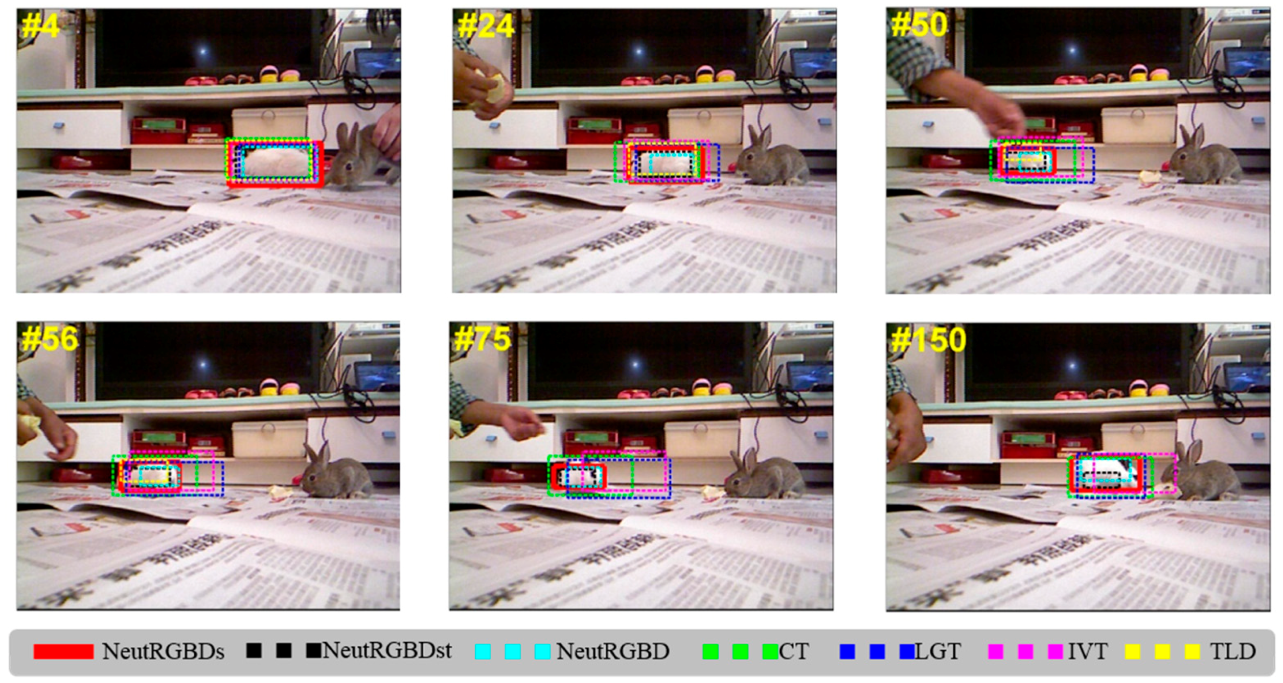
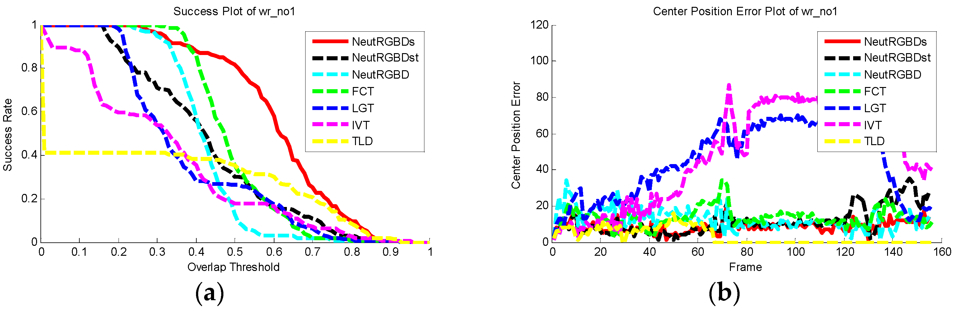
Wr_no1 sequence: This sequence highlights the challenges of rolling, blur, fast motion, and appearance change. As shown in Figure 1, all the trackers perform well until frame #24. However, the bounding box calculated by the NeutRGBD tracker has a relatively small scale. As seen in frames #50 and #56, only the NeutRGBDs tracker produces an adequate scale for the bounding box. As shown in frames #56, #75, and #150, a relatively small scale is estimated by the NeutRGBDst tracker. The CT, LGT, and IVT trackers failed to track the rabbit in frame #75 because of the wrongly estimated scale, and the TLD tracker failed due to the challenge of serious appearance change when the person tried to turn the rabbit back. As shown in Figure 5a, the NeutRGBDs tracker has a good success ratio when different overlap thresholds are selected. Due to the good performance when dealing with the scale adaption problem, the center location of the tracked object is closer to the ground truth in most frames, as seen in Figure 5b. In summary, during the whole tracking process, the NeutRGBDs tracker has the best performance.

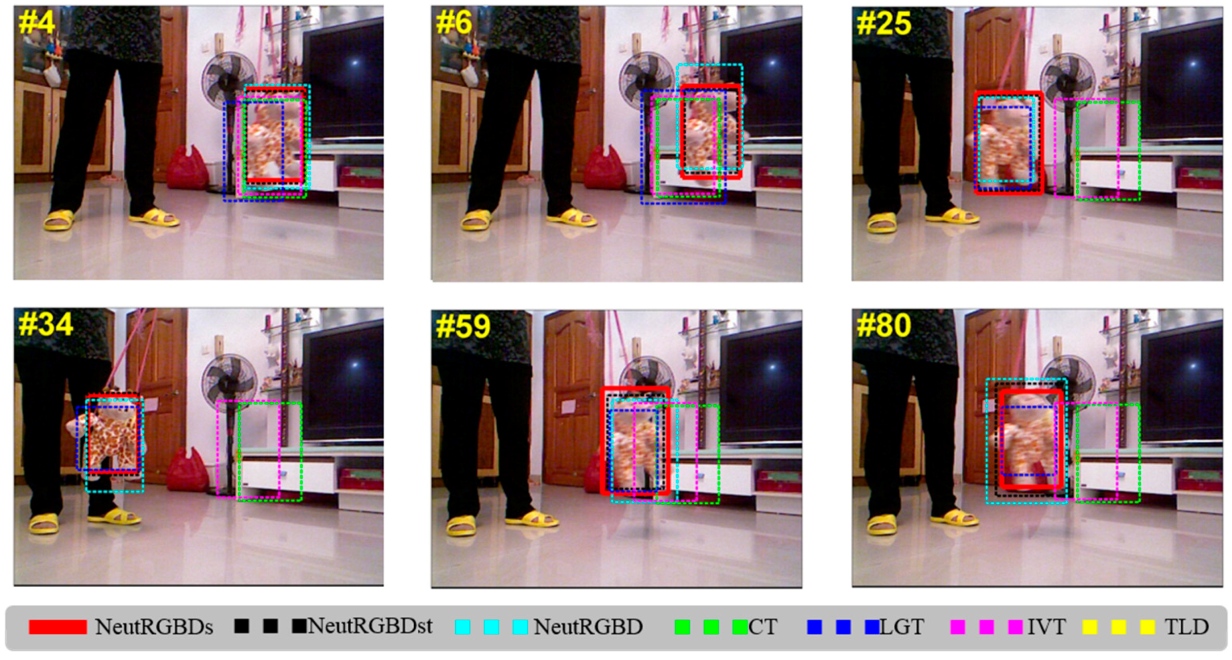
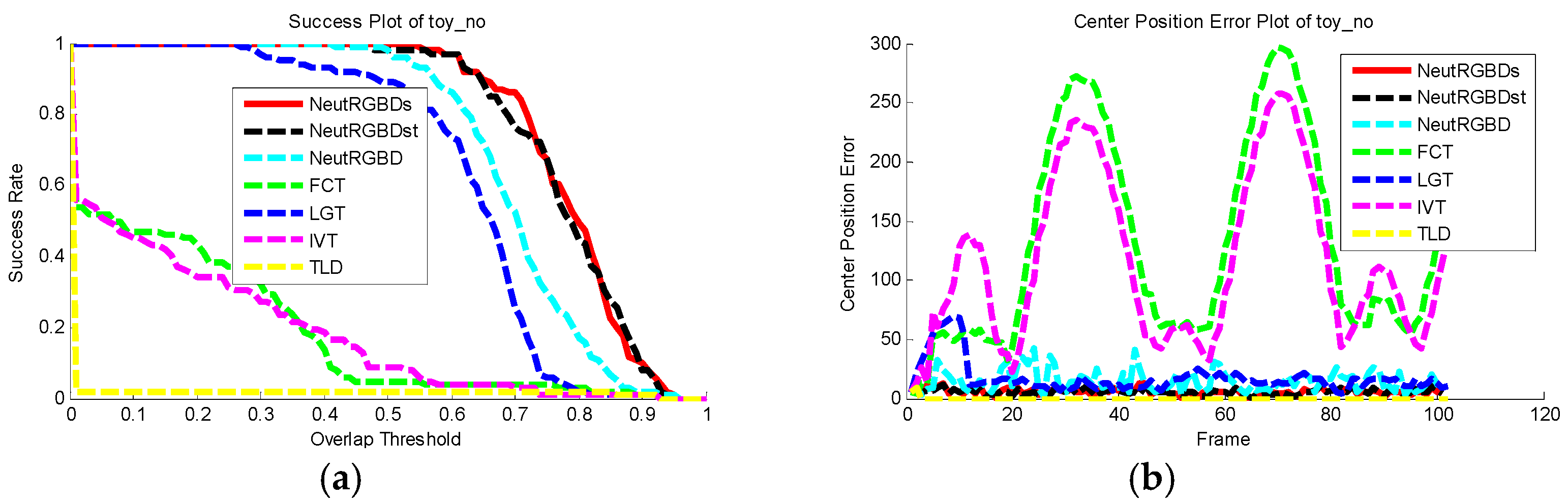
Toy_no sequence: The challenges like blur, fast motion, and rotation are included in this sequence. As seen in frame #6, the CT, IVT, and TLD trackers have already failed due to the fast motion of the toy. For the LGT tracker, an improper scale is estimated on account of the update of the local patches cannot follow such a rapid change. For the NeutRGBD tracker, due to the fact that the toy covers a relatively wide range of depth information, and the object seeds only cover a small range, the extracted object region sometimes only covers parts of the toy. As seen in Figure 6, on account of this factor, the center location of the target produced by the NeutRGBD tracker is less stable than that of the NeutRGBDs tracker. Thanks to the seed selection scheme, the NeutRGBDst tracker performs well on this sequence. Unlike the NeutRGBDs tracker, when calculating a neutrosophic correlation coefficient, T, I, and F are treated as the same weight for NeutRGBDst. As seen in Figure 2, the scale produced by the NeutRGBDs tracker performs the best. As shown in Figure 6a, both the NeutRGBDs and NeutRGBDst tracker perform well, and the NeutRGBDs tracker performs better when the overlap threshold is set to nearly 0.72.

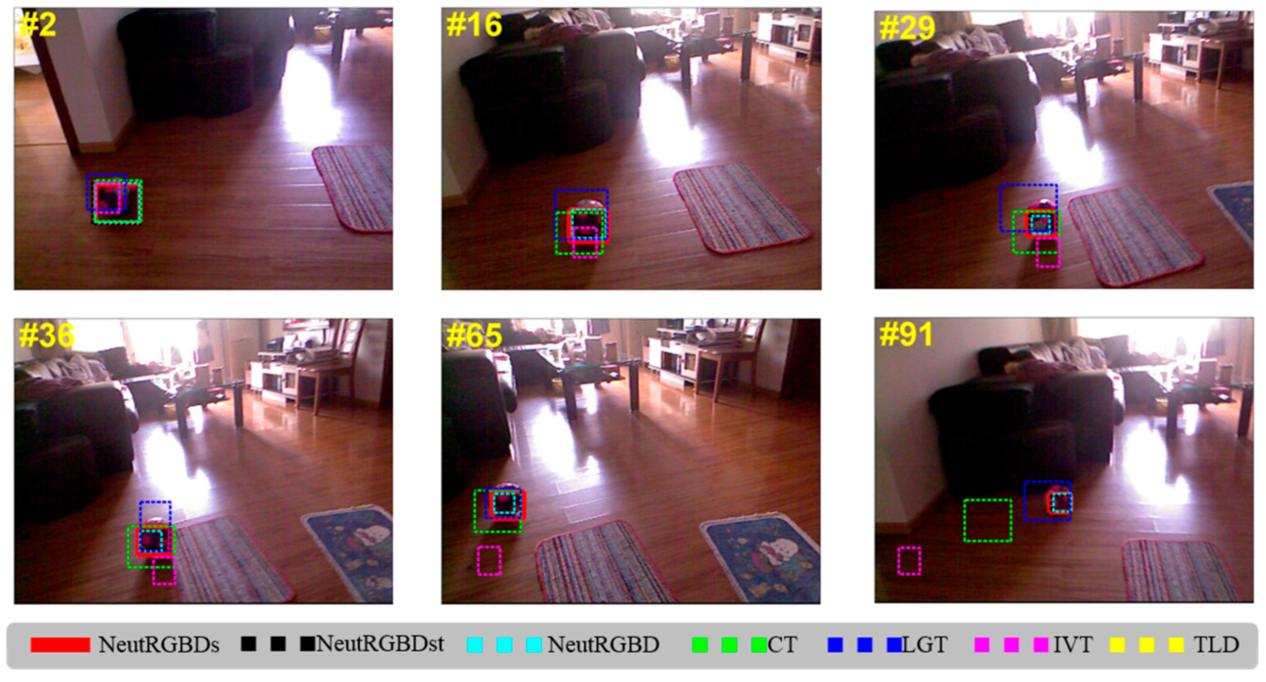
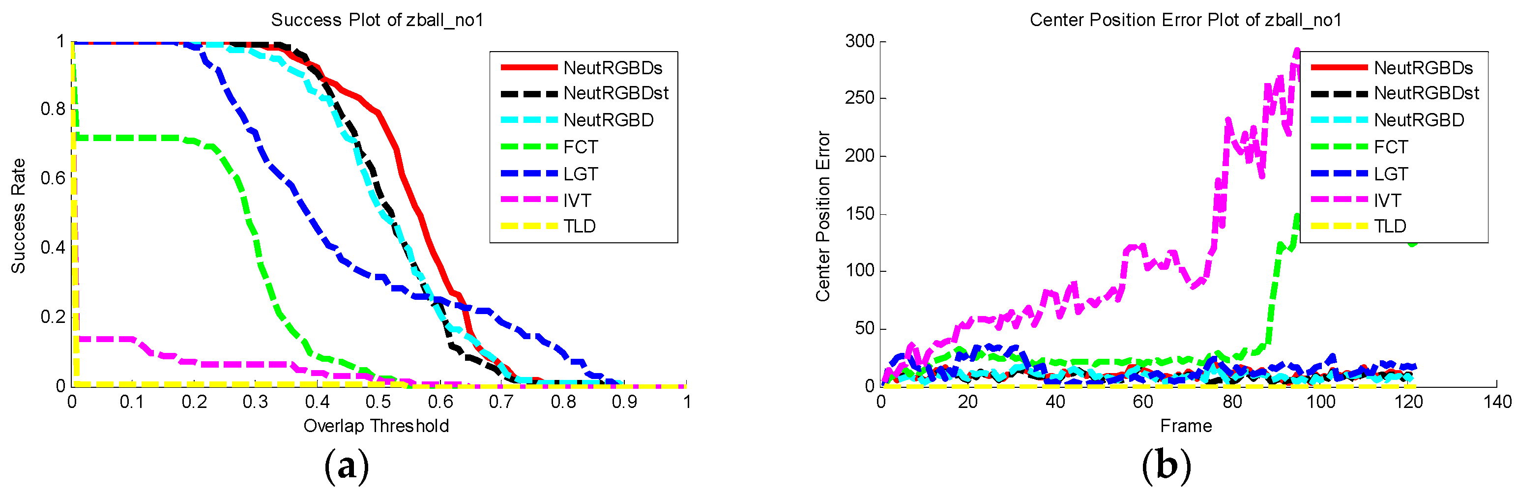
Zball_no1 sequence: Challenges of illumination variation, rapid motion and camera jitter existed in this sequence. Due to the challenge of appearance change and rapid motion, the TLD tracker fails soon, as seen in Figure 3. The IVT tracker also fails due to the similar surroundings, especially for the wood floor. Though a relatively large scale of the bounding box is estimated by the CT and LGT trackers, both of them can localize the ball properly before frame #65. With the challenges of similar surroundings, rapid motion, and camera jitter, the CT tracker has already failed before frame #91. As shown in Figure 7b, when judging the center position error evaluation criteria, owing to the information fusion in the neutrosophic domain, the NeutRGBDs, NeutRGBDst, and NeutRGBD tracker all perform well. Thanks to the scale adaption and seeds selection strategy, the NeutRGBDs tracker has a more appropriate scale than the other two, as seen in Figure 3 and Figure 7a.

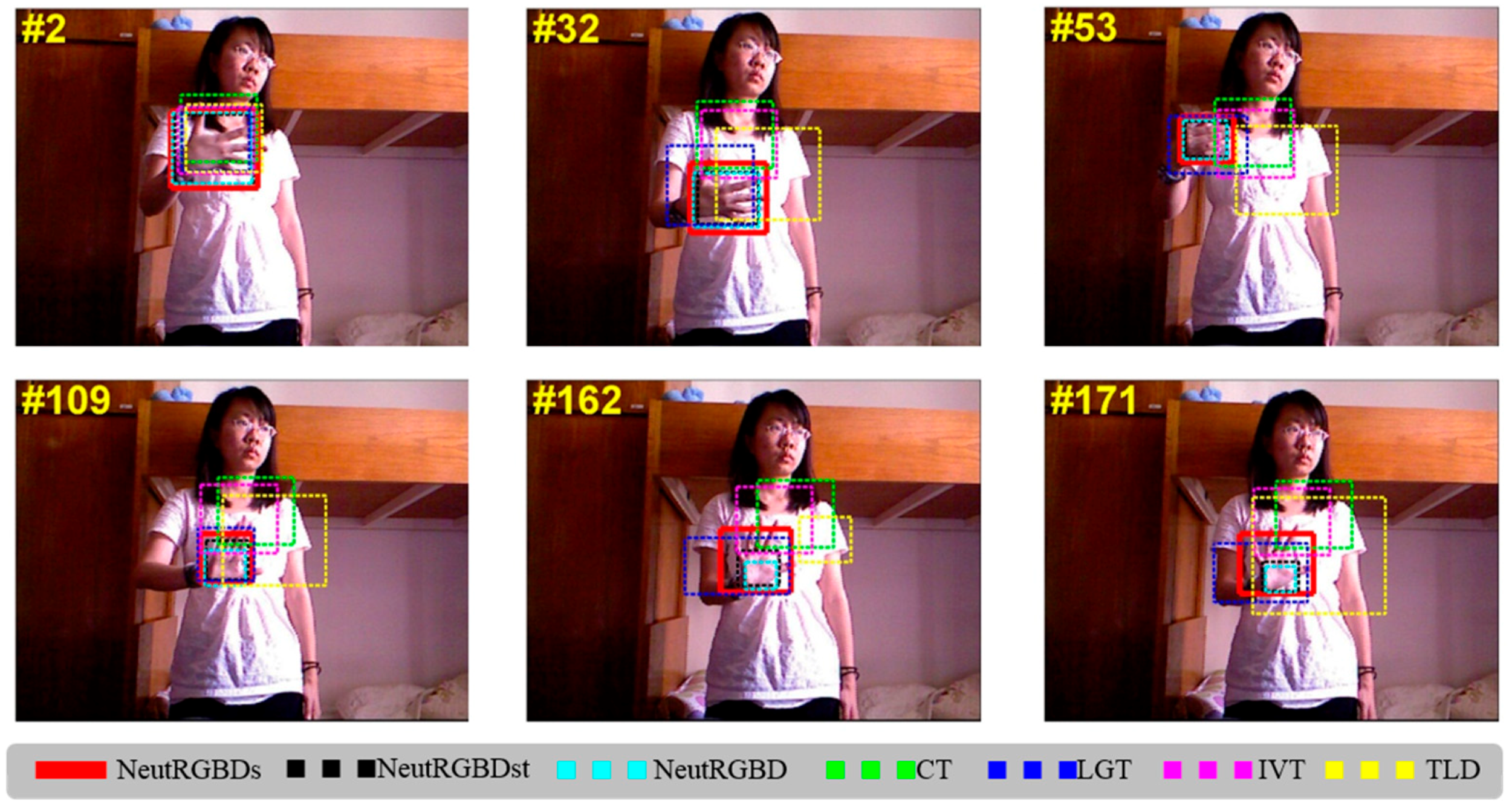
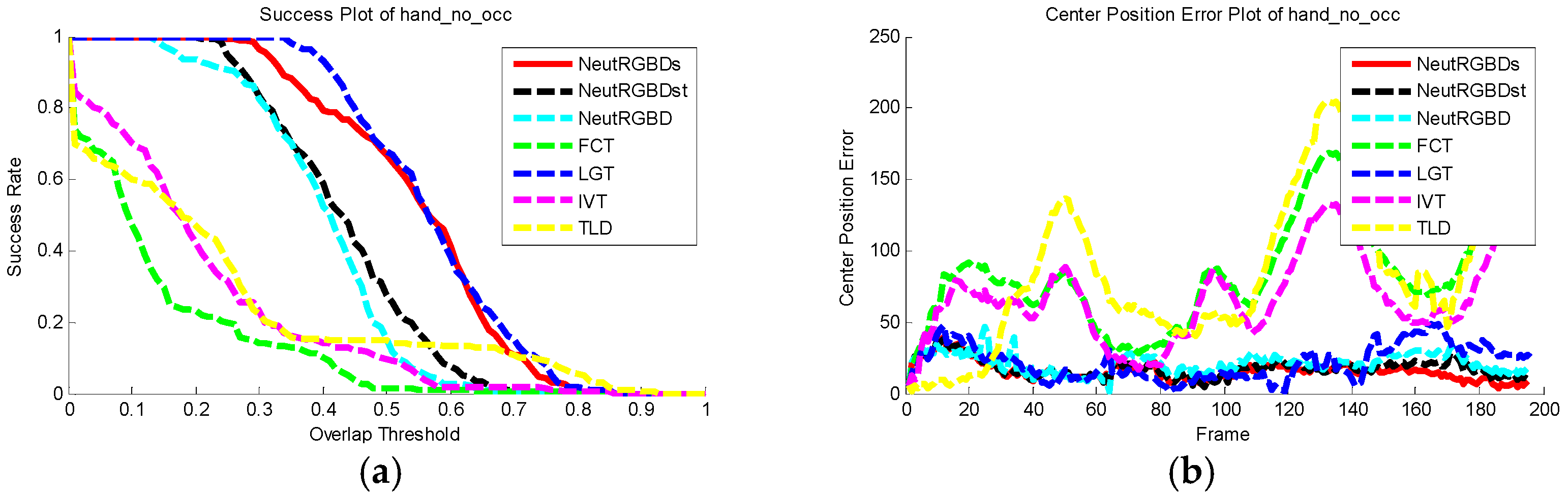
Hand_no_occ sequence: This sequence presents the challenges of illumination variation, deformation, out-of-plane rotation, and similar surroundings. As shown in frame #2 in Figure 4, a large background region is chosen as the object area at the phase of tracker initialization for the CT, LGT, IVT, and TLD tracker. All three trackers except LGT soon fail due to the weak initialization and the out-plane rotation challenge. The LGT tracker performs well throughout this sequence mainly due to the application of the scheme of apparent local motion. However, it is frequently disturbed by the similar surroundings, especially for regions with similar color and displacement. As seen in Figure 8b, a more accurate center has been produced by the NeutRGBDs tracker since frame #150. Although all three neutrosophic-based information fusion trackers perform well in this sequence, the NeutRGBDs tracker can produce a more accurate bounding box, as seen in Figure 4 and Figure 8.

4.4. Discussion

From the above illustrations of the tracking results, we see that a more accurate bounding box can be estimated when the element-weighted neutrosophic correlation coefficient is introduced into the CAMShift framework. Firstly, for the NeutRGBD tracker, only the depth information is considered for seed selection. A more robust seed selection scheme is applied by the NeutRGBDs tracker. Each seed is judged by using the T, I, and F elements in the neutrosophic domain, and the depth, color, and fused information are all taken into consideration. In addition, the truth element is emphasized for each criterion for the NeutRGBDs tracker. The object seeds play an essential role in the procedure of the NeutRGBD, NeutRGBDs, and NeutRGBDst tracker. The robust object seeds help the tracker earn a more accurate object region, as well as a more robust back-projection in the depth domain. Secondly, compared to the NeutRGBD tracker, the NeutRGBDs and NeutRGBDst trackers keep more useful information in both the color and depth domains in the final back-projection. Such a back-projection can provide a more discriminative feature when there are surroundings with similar color or depth to the target. Finally, for the NeutRGBDs and NeutRGBDst trackers, a scale identification process is first proposed in the neutrosophic domain, and this method contributes a lot when the CAMShift scheme fails to estimate an adequate scale. The only difference between the NeutRGBDs and NeutRGBDst trackers is the calculation of the correlation coefficient. The tangent correlation coefficient employed by the NeutRGBDst tracker treats the T, I, and F elements equally. As can be seen from the above analysis, it is the main reason the NeutRGBDs tracker always produces a more robust target bounding box.

5. Conclusions

A method of element-weighted neutrosophic correlation coefficient is proposed, and it is successfully applied in improving the CAMShift tracker in RGBD video. The experimental results have revealed its robustness. For the selection of robust object seeds, three kinds of criteria are proposed, and each candidate seed is represented in the SVNS domain via three membership functions, T, I, and F. Then these seeds are employed for extracting the object region and calculating the depth back-projection. Furthermore, the proposed neutrosophic correlation coefficient is applied for fusing the likelihood probability in both the color and depth domains. Finally, in order to modify the scale of the bounding box, two alternatives in the neutrosophic domain are proposed, and the corresponding correlation coefficient between the proposed alternative and the ideal one is employed for the identification of the scale. As discussed in this work, challenges without serious occlusion are considered here. It will be our primary mission to try to tackle the occlusion problem through the RGBD information in the future.

References

- Smarandache, F. Neutrosophy: Neutrosophic Probability, Set and Logic; American Research Press: Rehoboth, Delaware, 1998; p. 105. [Google Scholar]
- Wang, H.; Smarandache, F.; Zhang, Y.; Sunderraman, R. Single valued neutrosophic sets. Multisp. Multistruct. 2010, 4, 410–413. [Google Scholar]
- El-Hefenawy, N.; Metwally, M.A.; Ahmed, Z.M.; El-Henawy, I.M. A review on the applications of neutrosophic sets. J. Comput. Theor. Nanosci. 2016, 13, 936–944. [Google Scholar] [CrossRef]
- Ye, J.; Fu, J. Multi-period medical diagnosis method using a single valued neutrosophic similarity measure based on tangent function. Comput. Methods Programs Biomed. 2016, 123, 142–149. [Google Scholar] [CrossRef] [PubMed]
- Guo, Y.; Şengür, A. A novel image segmentation algorithm based on neutrosophic similarity clustering. Appl. Soft Comput. J. 2014, 25, 391–398. [Google Scholar] [CrossRef]
- Anter, A.M.; Hassanien, A.E.; ElSoud, M.A.A.; Tolba, M.F. Neutrosophic sets and fuzzy c-means clustering for improving ct liver image segmentation. Adv. Intell. Syst. Comput. 2014, 303, 193–203. [Google Scholar]
- Karabatak, E.; Guo, Y.; Sengur, A. Modified neutrosophic approach to color image segmentation. J. Electron. Imaging 2013, 22, 4049–4068. [Google Scholar] [CrossRef]
- Zhang, M.; Zhang, L.; Cheng, H.D. A neutrosophic approach to image segmentation based on watershed method. Signal Process. 2010, 90, 1510–1517. [Google Scholar] [CrossRef]
- Guo, Y.; Şengür, A.; Ye, J. A novel image thresholding algorithm based on neutrosophic similarity score. Meas. J. Int. Meas. Confed. 2014, 58, 175–186. [Google Scholar] [CrossRef]
- Guo, Y.; Sengur, A. A novel 3d skeleton algorithm based on neutrosophic cost function. Appl. Soft Comput. J. 2015, 36, 210–217. [Google Scholar] [CrossRef]
- Hu, K.; Ye, J.; Fan, E.; Shen, S.; Huang, L.; Pi, J. A novel object tracking algorithm by fusing color and depth information based on single valued neutrosophic cross-entropy. J. Intell. Fuzzy Syst. 2017, 32, 1775–1786. [Google Scholar] [CrossRef]
- Hu, K.; Fan, E.; Ye, J.; Fan, C.; Shen, S.; Gu, Y. Neutrosophic similarity score based weighted histogram for robust mean-shift tracking. Information 2017, 8, 122. [Google Scholar] [CrossRef]
- Biswas, P.; Pramanik, S.; Giri, B.C. Topsis method for multi-attribute group decision-making under single-valued neutrosophic environment. Neural Comput. Appl. 2015, 27, 727–737. [Google Scholar] [CrossRef]
- Kharal, A. A neutrosophic multi-criteria decision making method. New Math. Nat. Comput. 2014, 10, 143–162. [Google Scholar] [CrossRef]
- Ye, J. Single valued neutrosophic cross-entropy for multicriteria decision making problems. Appl. Math. Model. 2014, 38, 1170–1175. [Google Scholar] [CrossRef]
- Majumdar, P. Neutrosophic sets and its applications to decision making. In Adaptation, Learning, and Optimization; Springer: Cham, Switzerland, 2015; Volume 19, pp. 97–115. [Google Scholar]
- Ye, J. Multicriteria decision-making method using the correlation coefficient under single-valued neutrosophic environment. Int. J. Gen. Syst. 2013, 42, 386–394. [Google Scholar] [CrossRef]
- Baušys, R.; Juodagalvienė, B. Garage location selection for residential house by waspas-svns method. J. Civ. Eng. Manag. 2017, 23, 421–429. [Google Scholar] [CrossRef]
- Zavadskas, E.K.; Bausys, R.; Juodagalviene, B.; Garnyte-Sapranaviciene, I. Model for residential house element and material selection by neutrosophic multimoora method. Eng. Appl. Artif. Int. 2017, 64, 315–324. [Google Scholar] [CrossRef]
- Zavadskas, E.K.; Bausys, R.; Kaklauskas, A.; Ubarte, I.; Kuzminske, A.; Gudiene, N. Sustainable market valuation of buildings by the single-valued neutrosophic mamva method. Appl. Soft Comput. J. 2017, 57, 74–87. [Google Scholar] [CrossRef]
- Guo, Y.; Sengur, A. Ncm: Neutrosophic c-means clustering algorithm. Pattern Recognit. 2015, 48, 2710–2724. [Google Scholar] [CrossRef]
- Smeulders, A.W.M.; Chu, D.M.; Cucchiara, R.; Calderara, S.; Dehghan, A.; Shah, M. Visual tracking: An experimental survey. IEEE Trans. Pattern Anal. Mach. Intell. 2014, 36, 1442–1468. [Google Scholar] [PubMed]
- Wu, Y.; Lim, J.; Yang, M.H. Online object tracking: A benchmark. In Proceedings of the IEEE Conference on Computer Vision and Pattern Recognition (CVPR), Portland, OR, USA, 23–28 June 2013; pp. 2411–2418. [Google Scholar]
- Wang, X. Tracking Interacting Objects in Image Sequences; École Polytechnique Fédérale de Lausanne: Lausanne, Switzerland, 2015. [Google Scholar]
- Comaniciu, D.; Ramesh, V.; Meer, P. Kernel-based object tracking. IEEE Trans. Pattern Anal. Mach. Intell. 2003, 25, 564–577. [Google Scholar] [CrossRef]
- Bradski, G.R. Real time face and object tracking as a component of a perceptual user interface. In Proceedings of the Fourth IEEE Workshop on Applications of Computer Vision, Princeton, NJ, USA, 19–21 October 1998; pp. 214–219. [Google Scholar]
- Wong, S. An Fpga Implementation of the Mean-Shift Algorithm for Object Tracking; AUT University: Auckland, New Zealand, 2014. [Google Scholar]
- Leichter, I. Mean shift trackers with cross-bin metrics. IEEE Trans. Pattern Anal. Mach. Intell. 2011, 34, 695–706. [Google Scholar] [CrossRef] [PubMed]
- Zhu, C. Video Object Tracking Using Sift and Mean Shift. Master’s Thesis, Chalmers University of Technology, Gothenburg, Sweden, 2011. [Google Scholar]
- Bousetouane, F.; Dib, L.; Snoussi, H. Improved mean shift integrating texture and color features for robust real time object tracking. Vis. Comput. 2013, 29, 155–170. [Google Scholar] [CrossRef]
- Babenko, B.; Ming-Hsuan, Y.; Belongie, S. Visual tracking with online multiple instance learning. In Proceedings of the IEEE Conference on Computer Vision Pattern Recognition (CVPR), Miami, FL, USA, 20–25 June 2009; pp. 983–990. [Google Scholar]
- Hu, K.; Zhang, X.; Gu, Y.; Wang, Y. Fusing target information from multiple views for robust visual tracking. IET Comput. Vis. 2014, 8, 86–97. [Google Scholar] [CrossRef]
- Kaihua, Z.; Lei, Z.; Ming-Hsuan, Y. Fast compressive tracking. IEEE Trans. Pattern Anal. Mach. Intell. 2014, 36, 2002–2015. [Google Scholar]
- Cehovin, L.; Kristan, M.; Leonardis, A. Robust visual tracking using an adaptive coupled-layer visual model. IEEE Trans. Pattern Anal. Mach. Intell. 2013, 35, 941–953. [Google Scholar] [CrossRef] [PubMed]
- Ross, D.; Lim, J.; Lin, R.-S.; Yang, M.-H. Incremental learning for robust visual tracking. Int. J. Comput. Vis. 2008, 77, 125–141. [Google Scholar] [CrossRef]
- Kalal, Z.; Mikolajczyk, K.; Matas, J. Tracking-learning-detection. IEEE Trans. Pattern Anal. Mach. Intell. 2012, 34, 1409–1422. [Google Scholar] [CrossRef] [PubMed] [Green Version]
- Almazan, E.J.; Jones, G.A. Tracking people across multiple non-overlapping RGB-D sensors. In Proceedings of the IEEE Conference on Computer Vision and Pattern Recognition Workshops (CVPRW), Portland, OR, USA, 23–28 June 2013; pp. 831–837. [Google Scholar]
- Han, J.; Pauwels, E.J.; De Zeeuw, P.M.; De With, P.H.N. Employing a RGB-D sensor for real-time tracking of humans across multiple re-entries in a smart environment. IEEE Trans. Consum. Electr. 2012, 58, 255–263. [Google Scholar]
- Sridhar, S.; Oulasvirta, A.; Theobalt, C. Interactive markerless articulated hand motion tracking using rgb and depth data. In Proceedings of the IEEE International Conference on Computer Vision, Sydney, Australia, 1–8 December 2013; pp. 2456–2463. [Google Scholar]
- Camplani, M.; Hannuna, S.; Mirmehdi, M.; Damen, D.; Paiement, A.; Tao, L.; Burghardt, T. Real-time RGB-D tracking with depth scaling kernelised correlation filters and occlusion handling. In Proceedings of the British Machine Vision Conference (BMVC), Swansea, UK, 7–10 September 2015; pp. 145:1–145:11. [Google Scholar]
Figure 1.
Performance on “wr_no1” sequence by seven trackers.
Figure 2.
Performance on “toy_no” sequence by seven trackers.
Figure 3.
Performance on “zball_no1” sequence by seven trackers.
Figure 4.
Performance on “hand_no_occ” sequence by seven trackers.
Figure 5.
The quantitative plots for each tracker of the wr_no1 sequence: (a) Success plots; (b) center position error plots.
Figure 6.
The quantitative plots for each tracker of the toy_no sequence: (a) Success plots; (b) center position error plots.
Figure 7.
The quantitative plots for each tracker of the zball_no1 sequence: (a) Success plots; (b) center position error plots.
Figure 8.
The quantitative plots for each tracker of the hand_no_occ sequence: (a) Success plots; (b) center position error plots.