An Interactive Multiobjective Optimization Approach to Supplier Selection and Order Allocation Problems Using the Concept of Desirability

Abstract

In supply chain management, selecting the right supplier is one of the most important decision-making processes for improving corporate competitiveness. In particular, when a buyer considers selecting multiple suppliers, one should consider the issue of order allocation with supplier selection. In this article, an interactive multiobjective optimization approach is proposed for the supplier selection and order allocation problem. Also, the concept of desirability is incorporated into the optimization model to take into account the principles of diminishing marginal utility. The results are presented by comparing them with the solutions from the weighting methods. This study shows the advantage of the proposed method in that the decision-maker directly checks the degree of desirability and learns his/her preference structure through improved solutions.

1. Introduction

With the development of the Internet and network technologies, the digital divide between businesses is being addressed. In this situation, companies are using strategies to enhance outsourcing to focus on core competences along with information. In particular, such rapid developments in information technology are pushing many companies into a race that transcends time and space. Furthermore, the global business environment surrounding corporations is changing from competition between individual companies to competition between supply chains. In order to ensure the competitive edge of the supply chain, companies have tried to find the right suppliers offering higher quality, reduced costs, and shorter lead times. Therefore, in supply chain management, selecting the right suppliers is one of the most important decision-making processes for improving corporate competitiveness [1,2,3].

In many cases, a single supplier may not be able to meet the buyer’s requirements. In such cases, selecting multiple suppliers—multiple sourcing—would be a reasonable alternative [4]. Whereas single sourcing significantly increases the disruption risk in the supply chain, multiple sourcing increases the fixed cost in terms of administrative and negotiating costs [5]. However, multiple sourcing is preferred over a single sourcing, ensuring order flexibility [6]. Therefore, multiple sourcing inevitably includes the problem of order allocation. Furthermore, the relationship between the buyer and supplier is influenced by order allocation decisions based on strategic purchase decisions [7]. Therefore, the overall supplier selection problem should not only cover the selection of the right supplier but also the determination of the orders assigned to the selected supplier based on the given objectives and constraints [8]. To date, however, only a few mathematical programming models to analyze such decisions have been published [9,10,11,12]. In the field of supply chain management, it is necessary to develop a precise decision support model which simultaneously considers supplier selection and order allocation. In particular, researchers need to advance research in this direction to guide the decision-maker (DM)’s rational choice.

Supplier selection is inherently a multi-criteria decision-making (MCDM) problem since some conflicting performance criteria have an influence on the selection of suppliers [13,14]. It is also considered one of the most familiar problems in MCDM [15]. This problem has been studied from a variety of perspectives, such as green supplier selection [6,16] and global supplier selection [17]. Generally, the performance criteria involves the factors such as cost, quality, and lead time. Each supplier has its own strengths and weaknesses, so it is very difficult to select a superior supplier at all dimensions of criteria. Thus, supplier selection problem has made MCDM a very challenging task. Ho et al. [18] provided comprehensive reviews for MCDM approaches to vendor selection problems between 2000 and 2008. In addition, a more recent review from Chai et al. [19] provides guidelines for a MCDM-based supplier selection model.

For solving a multiobjective optimization (MOO) problem in MCDM, the DM seeks a compromise solution which provides the greatest satisfaction in the presence of conflicting objectives. Thus, the DM’s preference information plays a critical role in finding the solution. In the literature, the DM’s preference information can enter the solving process of MOO problems in three different ways: (1) a priori; (2) a posteriori; and (3) progressive (interactive) articulation [20,21]. For an a priori setting, multiple objective functions combined with preference convert into one single objective. For an a posteriori setting, the DM’s preference information is articulated after optimization process by selecting the most preferred one from a set of non-dominated solutions, usually called a Pareto optimal set. For progressive optimization, the preference of the DM is incorporated into the solution search process. Iterative dialogues between the DM and optimization model contribute to find the most satisfactory solution in this optimization approach. For this reason, the progressive articulation approach is also referred to as the interactive approach.

Most studies in supplier selection and order allocation are categorized into the prior approach by the MOO categorization scheme. However, the prior approach may decrease the reliability of solutions because of the unrealistic assumption that the DM can specify the preference information in advance. Although the interactive approach has been broadly applied to various fields as an alternative to overcome this limitation on the DM’s preference, it is rarely used to solve supplier selection and order allocation problems. To the best of the author’s knowledge, Demirtas and Üstün [4]’s research is the only material related to using the interactive MOO method to solve supplier selection and order allocation problem. Demirtas and Üstün [4] proposed an interactive MOO method, and a reservation level driven Tchebycheff procedure. In this model, the solution process makes the DM express adjusting some or all of reservation values of objective functions, by generating candidate solutions with sampling weights. The interactive method that we propose in this paper has something in common with Demirtas and Üstün [4]’s research in terms of a kind of objective space reduction. Also, two methods share the Tchebycheff framework to find a solution by utilizing the concept of distance to the ideal vector. However, the proposed approach provides an integrated use of the desirability function approach in response to surface methodology and the step method (STEM). Our model has advantages in that it reflects the satisfaction of the DM more realistically by using the concept of desirability function, and it reduces the burden on the DM to express preference information.

Based on the above-mentioned background, the purpose of the research is summarized as follows. We aim to solve the multiple sourcing problem which deals with order allocation at the same time as supplier selection by using an interactive MOO method. The devised method, which progressively articulates the DM’s preference information, is applied to a problem with three important criteria: cost, quality, and delivery. Also, to intuitively utilize the level of satisfaction, we borrow the concept of desirability from the research field of product and process design. We show that our method can be utilized effectively in the supplier selection and order allocation problem.

The organization of this paper is as follows. Section 2 presents previous works to be addressed in this study. The proposed interactive desirability function approach to supplier selection is presented in Section 3. Section 4 analyzes results and provides discussions. Conclusions are provided in Section 5.

2. Literature Review

This section briefly describes the concept of desirability function that is the basis for the proposed methodology. Then we deal with the consideration of the DM’s preference information in MOO problems. Also, the STEM is introduced.

2.1. Desirability Function Approach

The desirability function approach is in fact designed to solve the problem of product and process design (also called multiple response optimization). The desirability function approach, proposed by Harrington [22] and Derringer and Suich [23], is one of the most widely used methods in product and process design. This approach transforms an estimated response function into a scale-free function, called the desirability function, which ranges from zero to one. Thus, the value of the desirability function presents the degree of desirability or satisfaction for the corresponding response. If the larger-the-better (LTB) response is the objective that has to be maximized, the individual desirability function is defined as

$$d_i=\{\begin{array}{cc}0,& \mathrm{for}{\widehat{y}}_i(x)\le {\widehat{y}}_i^{\min }\hfill \\ {\left(\frac{{\widehat{y}}_i(x)-{\widehat{y}}_i^{\min }}{{\widehat{y}}_i^{\max }-{\widehat{y}}_i^{\min }}\right)}^r,& \mathrm{for}{\widehat{y}}_i^{\min }<{\widehat{y}}_i(x)<{\widehat{y}}_i^{\max }\hfill \\ 1,& \mathrm{for}{\widehat{y}}_i(x)\ge {\widehat{y}}_i^{\max },\hfill \end{array}$$

(1)

where ${\widehat{y}}_i^{\min }$ is the minimum and ${\widehat{y}}_i^{\max }$ is the maximum acceptable value of response i and r is the parameter (r > 0) that determines the shape of desirability functions. The function is convex if r > 1, and is concave if 0 < r < 1. If a response is of the smaller-the-better (STB) type, it is defined in a similar way to (1). Also, for a certain response, if the specified target value has to be attained, the response is referred to as the nominal-the-best (NTB) type. In this case, the individual desirability function is derived in a slightly different form from STB and LTB type. For more information, readers may refer to Derringer and Suich [23].

There are several ways to draw the optimal solution considering multiple individual desirability functions [22,23,24,25,26] but the most widely used method is to optimize by converting multiple desirability functions into single desirability. In most cases the concept of geometric means is often used for this aggregation.

2.2. Interactive Approach and Decision Maker’s Preference Information

The supplier selection is inherently a MCDM problem, since some conflicting criteria have influence on the selection of suppliers [13,14]. MOO is a mathematical optimization technique of MCDM, which involves more than one objective function to be optimized simultaneously. The ultimate goal of MOO is to find the best compromise solution from a set of the non-dominated solutions that satisfies multiple objectives simultaneously. Thus, it necessarily requires the involvement of the DM who provides the preference information among conflicting objectives. According to the timing of articulating the DM’s preference information, the MOO is classified into three categories: the prior approach, the posterior approach, and the interactive approach [20,21]. More detailed descriptions of the theories and applications of MOO studies can be found in the classical MOO textbooks: [20,27,28].

The interactive approach (also referred as the progressive approach) allows the DM to articulate his/her preference information progressively while solving the problem. The optimization process is repeated until the DM has found the most preferred solution to extracting preference information in an interactive manner. Specifically, at each iteration in an algorithm, the DM is asked to express some preference information given one or more solutions generated from the previous iteration. This information reflects the judgment based on the DM’s implicit value function, and the process updates the DM’s preference through adding the new information to an optimization model. Typically, a general interactive method has the following three steps [27].

• Step 1: Find an initial solution.
• Step 2: Interact with the DM.
• Step 3: Generate one or some new solution(s). If the DM is satisfied with the current solution, stop. Otherwise, go to step 2.

Over the years, a number of various interactive methods have been developed. The most well-known interactive methods are the step method (STEM) [29], the Geoffrion-Dyer-Feinberg (GDF) method [30], the Zionts-Wallenius (ZW) method [31], the reference direction approach (RDA) [32], and the Nondifferentiable Interactive Multiobjective BUndle-based optimization System (NIMBUS) [27]. Each of interactive methods has a different scheme from others in terms of which type of preference information is asked from the DM. No matter what kind of preference information is asked, an iterative process is valuable for the DM in that he/she can learn about the structure of the problem and expect the result of the interaction. Furthermore, each employs different computational algorithms. Therefore, a particular interactive method may be suitable for a specified MOO problem given mathematical properties or assumptions. In other words, there is no the sole interactive method that is decidedly superior to the others, in a universal sense. Even though a lot of extensions and variants of the interactive methods can be applied to the supplier selection problem, in this paper we propose an interactive approach based on the STEM with some modifications.

2.3. STEM

The STEM is proposed by Benayoun et al. [29] and it is known as the first interactive MOO method. Originally STEM is designed for the linear MOO problems, and it also can be applied to integer and nonlinear MOO problems [28]. The interactive process in the STEM begins with generating an initial feasible solution and identifying the ideal objective function values. The ideal objective function values are obtained by optimizing each individual objective function over the initial feasible region. At each iteration, the DM examines the current solution with the ideal objective function value, and presents his/her preference depending on the concept of level of satisfaction. In particular, the DM provides an amount of relaxation by which the objective function value can be sacrificed, in order to improve some other unsatisfied objectives. From this numerical information presented from the DM, it generates a new solution. If the DM satisfied with this new solution, this solution becomes a final solution as a compromise and the interactive process terminates. Otherwise this process is repeated until no further relaxation is accepted. The mathematical procedure for the STEM has been given in the following steps.

Step 0: Construct the pay-off table. In this step, the ideal objective function vector is obtained by maximizing each objective function individually. Let f^* be the ideal solution vector of the following K problems, $f^{*}=(f_1^{*},f_2^{*},\dots ,f_K^{*})$.

$$\begin{array}{l}{f}_i^{*}=\max f_i(x)\\ \mathrm{subject}\mathrm{to}\\ x\in S\end{array}$$

(2)

Step 1: Let h be iteration counter and set be zero (h = 0). Calculate π_i values for use in weighting the objectives:

$$\begin{array}{l}{\pi }_i=\{\begin{array}{l}\frac{f_i^{*}-n_i}{f_i^{*}}{\left[{\displaystyle {\sum }_{j=1}^n{c}_{ij}^2}\right]}^{-1/2},\mathrm{if}{f}_i^{*}>0,\\ \frac{n_i-f_i^{*}}{n_i}{\left[{\displaystyle {\sum }_{j=1}^n{c}_{ij}^2}\right]}^{-1/2},\mathrm{if}{f}_i^{*}\le 0,\end{array}\\ \end{array}$$

(3)

where c_ij are the coefficients of the ith objective. The first term is to place the most weight on the objectives with the greatest relative ranges. The second term normalizes the gradients of the objective functions.

Step 2: Let h = h + 1, and S^h+1 = S. S¹ = S means the solution process begin with the original feasible region. At this point, the relaxation index set be null (J = ∅). Compute relative weights:

$${\lambda }_i^h=\{\begin{array}{l}0,i\in J\\ \frac{{\pi }_i}{{\displaystyle {\sum }_j{\pi }_j}},i\notin J\end{array}$$

(4)

Step 3: Solve the weighted minimax program:

$$\begin{array}{l}\min \alpha \\ \mathrm{subject}\mathrm{to}\\ \alpha \ge {\lambda }_i^h\left[f_i^{*}-f_i(x)\right],i=1,\dots ,k\\ x\in S^h\\ \alpha \ge 0\end{array}$$

(5)

If all objective function values are satisfactory, then stop; the current solution may become the final solution.

Step 4: Determine satisfactory objective and then specify the amount of relaxation, Δ_i (i ∈ J).

Step 5: Form reduced feasible region:

$$S^{h+1}=\{\begin{array}{l}x\in S\hfill \\ f_i(x)\ge f_i(x^h),i\notin J\hfill \\ f_i(x)\ge f_i(x^h)-{\Delta }_i,i\in J\hfill \end{array}$$

(6)

where h + 1 is increased iteration counter. Thus, $S^{h+1}$ is the feasible region in the (h + 1)th iteration. f_i(x)^h is the objective function value in the hth iteration and Δ_i is the amount of relaxation of particular objective function. Go to Step 2 with the reduced feasible region.

The STEM is widely used to solve not only linear but also nonlinear MOO problems for the reason that it is simple and straightforward to generate the solution by reducing feasible regions in the objective space. Despite these advantages, the STEM shows two major drawbacks. First, the STEM does not take into account different degrees of satisfaction within the acceptable interval of a relaxed objective. For example, suppose that one objective f_e is determined by the DM as a satisfactory function, and that he/she decides to relax as much as the Δ_e. In this case, the weight of objective function e becomes zero since e ∉ J, so this function does not serve as an objective function in the next iteration. Therefore, the solution of the next iteration depends on the assumption that the satisfaction of the DM is indifferent within the interval of [f_e − Δ_e, f_e^*]. This disadvantage has been pointed out by Jeong and Kim [33]. The second drawback is in the dialogue scheme between the DM and the optimization model. The dialogue is made mainly by asking the DM to acceptable amount of relaxation of a satisfactory objective. However, it increases the burden on the DM because he/she must provide specific numerical information at each iteration. In this paper, we intend to utilize the STEM to supplier selection problem by modifying it in such a way that we enjoy its merits and complement the shortcomings mentioned above. More specifically, we try to overcome the first limitation by applying the concept of desirability function and the second one by proposing a modification to the DM’s preference information representation.

3. Proposed Model

Across fifty years of evaluating suppliers, many researchers have proposed different sets of criteria.

The first set of criteria was proposed by Dickson [14], who identified 23 different criteria evaluated in supplier selection. Evans [34] and Shipley [35] agreed that price, quality and delivery are the most important criteria for evaluating suppliers. Ellram [36] proposed that the quality dimension should be divided into product quality and service quality, and it is suggested to use them with price and delivery time to select suppliers. Weber et al. [37] surveyed based on Dickson’s 23 criteria and concluded that price, delivery, quality, production capacity, and localization are the most important criteria. Pi and Low [38] proposed quality, delivery, price and service for supplier evaluation. Amid et al. [39] uses price, quality, and service, and Jadidi et al. [11] utilized price, quality, and lead time to the supplier selection and order allocation model. As shown by the literature, the most important criteria for supplier selection problems are cost, quality, and delivery. We also use those criteria by using the measures: total purchasing costs, the number of rejects, and the number of late delivery for cost, quality, and delivery, respectively. We assume the buyer considers a single item that should be purchased under known total demand. Also, information about criteria and production capacity is already known for a set of potential suppliers. The notations of the proposed model are presented in

Table 1. The notations.

k	index for objectives, k = 1, 2, …, K
n	number of suppliers
xi	number of units ordered to supplier i (decision variable)
x	vector of decision variables
Vi	capacity of supplier i
ci	unit purchasing price from supplier i
qi	expected defect rate of supplier i
li	percentage of items delivered late by supplier i
D	demand

.

There are three original objective functions: f₁ (minimizing total purchasing cost), f₂ (minimizing total number of defects), f₃ (minimizing the number of late delivery). Each objective function can be shown as follows:

$$\begin{array}{l}{f}_1(x)={{\displaystyle {\sum }_i^{n}c}}_i{x}_i\\ f_2(x)={{\displaystyle {\sum }_i^{n}q}}_i{x}_i\\ f_3(x)={\displaystyle {\sum }_i^n{l}_i}{x}_i\end{array}$$

(7)

Using the functions defined above, MOO problem considering the supplier selection with order allocation can be formulated as follows [12]:

$$\begin{array}{l}\min f_1(x),f_2(x),f_3(x)\\ \mathrm{subject}\mathrm{to}\\ {\displaystyle {\sum }_i^n{x}_i}=D\\ x_i\le V_i\\ x_i\ge 0\end{array}$$

(8)

The first and second constraint present demand satisfaction and capacity restriction, respectively, and the last constraint ensures non-negativity of the decision variables. Now we transform the original objective functions into the desirability functions. Because all original objective functions are to be minimized (STB type), the individual desirability is defined as

$$d_i=\{\begin{array}{cc}1,\hfill & \mathrm{for}{f}_i(x)\le f_i^{*}\hfill \\ {\left(\frac{f_i(x)-f_i^{\max }}{f_i^{*}-f_i^{\max }}\right)}^r,\hfill & \mathrm{for}{f}_i^{*}<f_i(x)\le f_i^{\max }\hfill \\ 0,\hfill & \mathrm{for}{f}_i(x)\ge f_i^{\max },\hfill \end{array}$$

(9)

where f_i^max are the maximum values of the objective functions as obtained from the payoff table and f_i^*(x) are the ideal points from maximizing the objective functions individually.

Table 2. Payoff table.

Payoffs	f1	f2	f3
f1	58.75	5.325	3.675
f2	82.25	3.225	5.05
f3	61.25	5.07	3.425

presents the payoff table that includes f_i^max and f_i^*(x). For a STB type function, f_i^max are recognized as the nadir points which are maximum values from each column in the payoff table, and the ideal values are on the diagonal of the table.

We represent the desirability-based supplier selection problem in the form of a MOO problem:

$$\begin{array}{l}\max d_1(f_1(x)),d_2(f_2(x)),d_3(f_3(x))\\ \mathrm{subject}\mathrm{to}\\ {\displaystyle {\sum }_i^n{x}_i}=D\\ x_i\le V_i\\ x_i\ge 0\end{array}$$

(10)

The individual desirability functions d_i (i = 1, …, k) are objective functions to be maximized simultaneously.

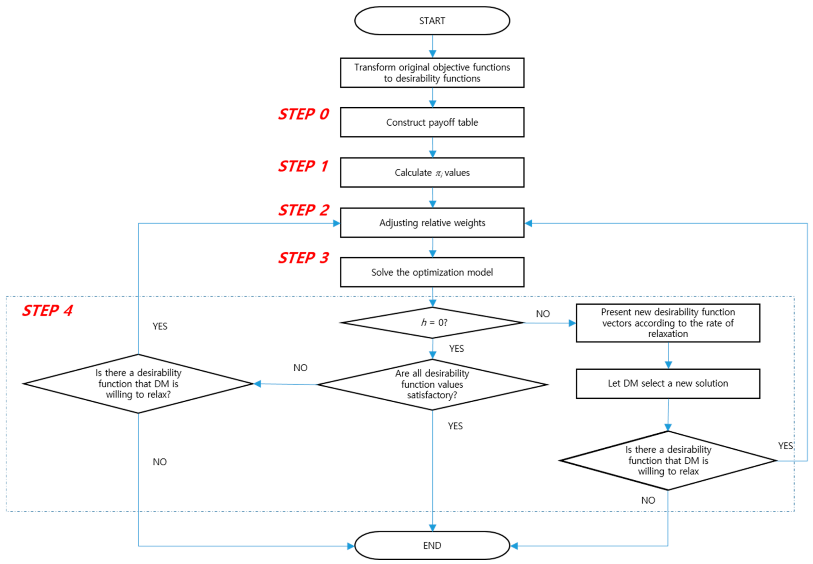
The optimization process consists of five major steps. The overall procedure is presented in Figure 1. In addition, a pseudo code is described in Algorithm 1 to aid readers understanding.

Algorithm 1. Pseudo code of the proposed method.
begin
	initialize: h ← 0
	initialize: J = ∅
	calculate d* and n*
	calculate πi values
	compute relative weights ${\lambda }^{\underset{\_}{h}}$
	compute an initial solution dh
	ask if there is a desirability function value want to relax (j)
	while the preferred solution has not been found do
		J = {j}
		compute relative weights ${\lambda }^{\underset{\_}{h}}$
		compute potential solutions based on the preferences of the DM
		present the solutions to the DM
		ask the most preferred solution dh* from potential solutions
		ask if there is a desirability function value want to relax (j)
		h ← h + 1
	endwhile
end

3.1. Case r = 1

We apply a modified STEM to supplier selection problem. In order to present how the method works, we deal with the linear type desirability function transformation.

3.1.1. Initialization

Step 0: Construct the payoff table (

Table 3. Payoff table of r = 1.

Payoffs	d1	d2	d3
d1	1	0	0.846
d2	0	1	0
d3	0.894	0.119	1

) based on the desirability functions with r = 1.

Therefore, the ideal vector and nadir vector are d* = (1, 1, 1) and n* = (0, 0, 0), respectively.

Step 1: Calculate π_i values for use in weighting the objectives: The coefficients c_ij, which reflect the gradients of the objective functions in the weight calculation is the coefficient of desirability function, not the original objective function. If the desirability functions are nonlinear, i.e., r ≠ 1, the weights calculation is somewhat different from that of the linear case. As mentioned in Section 2.2, originally the STEM is developed for multiobjective linear problems, but nonlinear extensions have been proposed, for example, in Vanderpooten and Vincke [40], Eschenauer et al. [41], and Sawaragi et al. [42]. A weight calculation scheme for the nonlinear case (r = 2) is presented in following Section 3.2. At this point, calculated π_i values are shown as

$$\begin{array}{l}{\pi }_1=\frac{d_1^{*}-n_1}{d_1^{*}}{\left[{\displaystyle {\sum }_j{c}_{1j}^2}\right]}^{-1/2}=2.1588\\ {\pi }_2=2.6158\\ {\pi }_3=2.3039\end{array}$$

Step 2: Let h be iteration counter (set h as zero for the first iteration).

For h = 0, the relaxation index set be null (J = ∅).

S⁰ = S, the original feasible region. Compute relative weights:

$$\begin{array}{l}{\lambda }_1^{h=0}={\pi }_1/({\pi }_1+{\pi }_2+{\pi }_3)=0.3050\\ {\lambda }_2^0=0.3695\\ {\lambda }_3^0=0.3255\end{array}$$

Step 3: Formulate the weighted minimax program:

$$\begin{array}{l}\min \alpha \\ \mathrm{subject}\mathrm{to}\\ \alpha \ge 0.3050(1-d_1)\\ \alpha \ge 0.3695(1-d_2)\\ \alpha \ge 0.3255(1-d_3)\\ {\displaystyle {\sum }_i^n{x}_i}=D\\ x_i\le V_i\\ x_i\ge 0\\ \alpha \ge 0\end{array}$$

(11)

The obtained solution is d^0* = (d₁^0*, d₂^0*, d₃^0*) = (0.4867, 0.5755, 0.5181). We assume the DM does not satisfied with the obtained solution. Go to Step 4.

Step 4: Determine satisfactory objective by asking the DM to express satisfactory objectives. If h = 0, go to Step 2 by setting h = h + 1. We assume the DM satisfied with d₂, so relax d₂.

3.1.2. First Iteration

Step 2: Compute relative weights (h = 1, S¹ = S): For h = 1, the objective function to be relaxed has been defined as d₂, thus {2} = J. Accordingly, the computed weights are ${\lambda }_1^1$ = π₁/(π₁ + π₃) = 0.4847, ${\lambda }_2^1$ = 0, and ${\lambda }_3^1$ = 0.5163.

Step 3: Formulate the weighted minimax program:

$$\begin{array}{l}\min \alpha \\ \mathrm{subject}\mathrm{to}\\ \alpha \ge 0.4837(1-d_1(x))\\ \alpha \ge 0.5163(1-d_3(x))\\ d_1(x)\ge d_1^{0*}\\ d_2(x)\ge (1-\delta )d_2^{0*}\\ d_3(x)\ge d_3^{0*}\\ {\displaystyle {\sum }_i^n{x}_i}=D\\ x_i\le V_i\\ x_i\ge 0\\ \alpha \ge 0\end{array}$$

(12)

where $\delta$ is rate of relaxation.

Step 4: Present new desirability function vectors to the DM as shown in

Table 4. Changes of desirability function values according to the rate of relaxation (h = 1).

	δ = 0.05	δ = 0.10	δ = 0.15	δ = 0.20	δ = 0.25	δ = 0.30
d1	0.511	0.537	0.563	0.589	0.614	0.640
d2	0.547	0.518	0.489	0.460	0.432	0.403
d3	0.542	0.566	0.590	0.615	0.639	0.663

, who is asked to select an acceptable rate of relaxation, δ. Unlike original STEM, the proposed approach does not compel the DM to ask specified amount of relaxation from satisfactory level. Then, the optimal solution corresponding selected rate of relaxation becomes the new vector of desirability function values.

If the DM is satisfied with the new solution with selected rate of relaxation, δ*, then stop. Otherwise, set h = h + 1 and set the new feasible reason S^h+1. Go to Step 2. Assume the DM choose 20% relaxation of d₂. Therefore, a new solution is d^1* = (0.589, 0.460, 0.615) with f = (61.167, 5.083, 3.582). Also, we assume the DM satisfied with d₁, and relax d₁.

3.1.3. Second Iteration

Step 2: Let h = 2. Compute relative weights: ${\lambda }_1^2=0,{\lambda }_2^2=0.5317,{\lambda }_3^2=0.4683$.

Step 3: Formulate the weighted minimax program:

$$\begin{array}{l}\min \alpha \\ \mathrm{subject}\mathrm{to}\\ \alpha \ge 0.5317(1-d_2(x))\\ \alpha \ge 0.4683(1-d_3(x))\\ d_1(x)\ge (1-\delta )d_1^{1*}\\ d_2(x)\ge d_2^{1*}\\ d_3(x)\ge d_3^{1*}\\ {\displaystyle {\sum }_i^n{x}_i}=D\\ x_i\le V_i\\ x_i\ge 0\\ \alpha \ge 0\end{array}$$

(13)

Step 4: As shown in

Table 5. Changes of desirability function values according to the rate of relaxation (h = 2).

	δ = 0.05	δ = 0.10	δ = 0.15	δ = 0.20	δ = 0.25	δ = 0.30
d1	0.559	0.530	0.500	0.471	0.441	0.412
d2	0.493	0.526	0.550	0.573	0.596	0.619
d3	0.626	0.614	0.614	0.614	0.614	0.614

, present new desirability function vectors as δ increases, then ask to the DM an acceptable rate of relaxation, δ.

Assume the DM choose 15% relaxation of d₁. Accordingly, a new solution is d^2* = (0.500, 0.550, 0.614) with f = (70.494, 4.170, 4.052). This interactive process can be repeated until the final solution satisfies the DM. At this stage, we assume that the DM is satisfied with the current solution and terminate the iterative procedure.

3.2. Case r = 2

All three original objective functions considered in the supplier selection model are linear, and the defined desirability functions in Section 3.1 are also linear. This sub-section discusses the need for nonlinear desirability functions and presents a problem-solving process in r = 2 case.

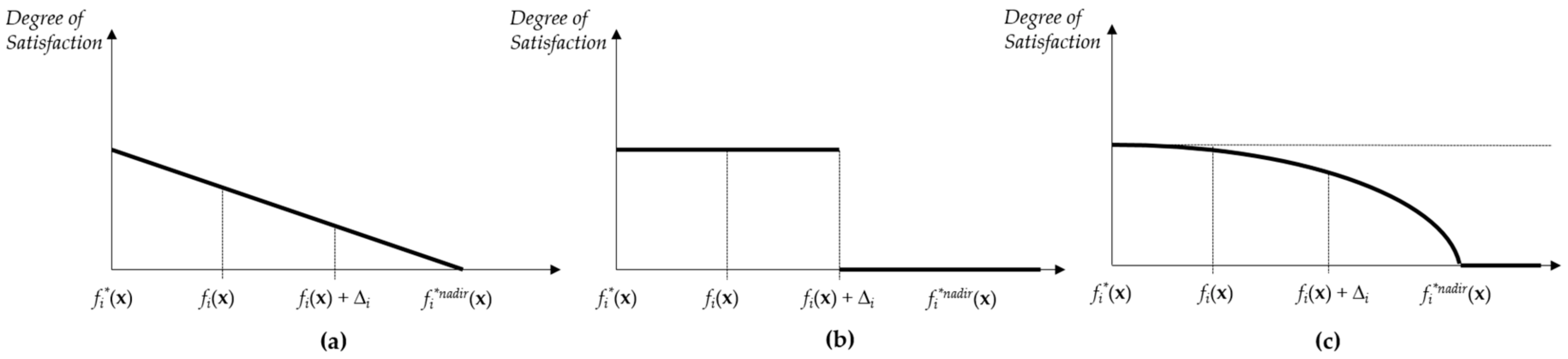
The weighted sum method assumes that the DM’s overall desirability (utility) is determined by the weighted sum of multiple objective functions. Thus, the marginal contribution to utility of each linear objective function is constant (see Figure 2a). Therefore, the optimization result is highly dependent upon the predetermined weights, although the objective functions are normalized by using the ideal points and the nadir points. On the other hand, the STEM modifies the concept of satisfaction by accepting the DM’s preference information in the problem-solving process. In particular, the STEM assumes that the desirability of the DM is the same up to the acceptable level, i.e., f_i(x) + Δ_i for a STB type objective function (see Figure 2b). Namely, the STEM considers that the DM’s satisfaction is indifferent within the interval of [f_i^*, f_i(x) + Δ_i]. With this concept the STEM improves the other objective functions at a level that does not impair the satisfaction of the satisfactory objective. However, we need to consider the principles of diminishing marginal utility, overlooked in the STEM. The principles of diminishing marginal utility explain that the closer the objective function value is to the optimum value, the less contribution it will make. In this study, the desirability function enables the proposed model to consider the principles of diminishing marginal utility. If the parameter r of desirability functions is not equal to 1, the functions become nonlinear. The parameter r exhibits a diminishing marginal contribution to the maximum cumulative desirability. The nonlinearity of desirability function provides a clue to successfully deal with the principles of diminishing marginal utility in the proposed model. This characteristic is also highlighted in Jeong and Kim [33]’s STEM based on the desirability function. Figure 2c shows an example of a nonlinear desirability function.

3.2.1. Initialization

Step 0: Construct the payoff table (

Table 6. Payoff table of r = 2.

Payoffs	d1	d2	d3
d1	1	0	0.799
d2	0	1	0.014
d3	0.716	0	1

) based on the desirability functions with r = 2.

Therefore, the ideal vector and nadir vector are d* = (1, 1, 1) and n* = (0, 0, 0.014), respectively.

Step 1: Calculate π_i values for use in weighting the objectives. The several weight schemes used to extend the STEM to nonlinear MOO problems were suggested by various researchers (Eschenauer et al. [41]; Sawaragi et al. [42]; Vanderpooten and Vincke [40]). In this study, we utilize Vanderpooten and Vincke [40]’s calculation (assume that the denominators are not equal to zero) as follows:

$${\pi }_i=\frac{d_i^{*}-n_i}{\max \{d_i^{*},n_i\}},$$

(14)

By (14), the determined weights are π₁ = π₂ = 1 and π₃ = 0.986.

Step 2: Compute relative weights: ${\lambda }_1^0={\lambda }_2^0=0.3349$, ${\lambda }_3^0=0.3302$

Step 3: Solve the weighted minimax program: d^0* = (0.2789, 0.2789, 0.3622).

Step 4: We assume the DM satisfied with d₂, so relax d₂. Go to Step 2.

3.2.2. First Iteration

Step 2: Compute relative weights (h = 1, S¹ = S): For h = 1, the objective function to be relaxed has been defined as a d₂, {2} = J. Thus, the computed weights are ${\lambda }_1^1$ = 0.5035, ${\lambda }_2^1$ = 0, and ${\lambda }_3^1$ = 0.4965.

Step 3 and Step 4: Solve the weighted minimax program and present new desirability function vectors as δ increases, then ask to the DM an acceptable rate of relaxation, δ. Use the computation results as shown in

Table 7. Changes of desirability function values according to the rate of relaxation (h = 1).

	δ = 0.05	δ = 0.10	δ = 0.15	δ = 0.20	δ = 0.25	δ = 0.30
d1	0.292	0.305	0.319	0.334	0.350	0.366
d2	0.265	0.251	0.237	0.223	0.209	0.195
d3	0.362	0.362	0.362	0.362	0. 362	0.362

.

Assume the DM choose 10% relaxation of d₂. Therefore, a new solution is d^1* = (0.305, 0.251, 0.362) with f = (69.271, 4.273, 4.072). We assume the DM satisfied with the current solution, and terminate the procedure.

4. Summary of Results and Discussion

This study successfully applied the concept of desirability function in response surface methodology, which is used in product and process design, to supplier selection problems. The desirability function diverts the DM’s recognition system for each objective function from linear coupling and realistically reflects the degree of satisfaction for each objective function. Since the proposed method assumes that the DM’s preference information is not completely known, it is difficult to discuss the superiority of solutions by directly comparing the results with other methods. However, we explain the advantages of the proposed method by comparing them with the solutions from two weighting methods: the weighted sum method and weighted geometric method. Several weighting vectors are assumed for the purpose of comparing solutions. We adopted three sets of weighting parameter w, proposed be Jadidi et al. [11] for the same supplier selection problem. The results are shown in

Table 8. Comparison with some weighting methods.

	w	d	x	f
Weighted sum	0.33, 0.33, 0.33	0.894, 0.119, 1.000	5, 1.5, 3.5, 6, 0, 0	61.250, 5.075, 3.425
	0.60, 0.20, 0.20	1.000, 0.000, 0.846	5, 4, 3.5, 3.5, 0, 0	58.750, 5.325, 3.675
	0.80, 0.10, 0.10	1.000, 0.000, 0.846	5, 4, 3.5, 3.5, 0, 0	58.750, 5.325, 3.675
Weighted geometric mean	0.33, 0.33, 0.33	0.577, 0.409, 0.878	3.8, 0, 3.5, 6, 0, 2.7	68.695, 4.467, 3.623
	0.60, 0.20, 0.20	0.798, 0.226, 0.908	5, 0, 3.5, 6, 1.5, 0	63.500, 4.850, 3.575
	0.80, 0.10, 0.10	0.894, 0.119, 1.000	5, 1.5, 3.5, 6, 0, 0	61.250, 5.075, 3.425
Overall desirability function1	r = 1	0.577, 0.409, 0.878	3.8, 0, 3.5, 6, 0, 2.7	68.695, 4.467, 3.623
	r = 2	0.333, 0.167, 0.771	3.8, 0, 3.5, 6, 0, 2.7	68.695, 4.467, 3.623
Proposed method	r = 1, h = 0	0.487, 0.576, 0.518	1.4, 0, 3.5, 5.6, 5.5, 0	70.836, 4.116, 4.197
	r = 1, h = 1	0.589, 0.460, 0.615	2.5, 0, 3.5, 6, 4, 0	68.419, 4.358, 3.943
	r = 1, h = 2	0.500, 0.550, 0.614	1.7, 0, 3.5, 6, 4.4, 0.4	70.494, 4.170, 4.052
	r = 2, h = 0	0.279, 0.279, 0.363	0.5, 1.7, 3.5, 6, 4.2, 0	69.840, 4.216, 4.072
	r = 2, h = 1	0.305, 0.251, 0.362	2.2, 0, 3.4, 5.8, 4.6, 0	69.271, 4.273, 4.072

¹ A special case of weighted geometric mean with equal weights.

.

The results of the weighted sum method show that the more weights are assigned to the first objective function (minimizing total purchasing costs), the larger the contribution is made to the value of the first desirability function. However, when w₁ is larger than 0.6, the individual desirability value for f₂ equals to 0. Namely, the second objective function, the number of late delivery, has the worst value. Furthermore, there is no differences between w = (0.6, 0.2, 0.2) and w = (0.8, 0.1, 0.1), although the overall objective function values ∑w_id_i differ. These extreme results show that the DM may not satisfied with the results.

Next, we also tested the weighted geometric model using the same set of w. In fact, the weighted geometric mean is a popular method for unifying individual desirability functions to a single function in desirability function approach. The weighted geometric method results in a somewhat balanced solution avoiding extreme values in one objective function, even if the weight is to one side. This method, however, also may result in a controversial solution. In Table 8, we found the third desirability value for late delivery increases as w₃ decreases. Thus, the results do not necessarily guarantee that the DM can find the most satisfactory solution even if he/she can decide preference information in advance at one time. The proposed method can complement the shortcomings of these methods because the DM directly checks the degree of desirability and learns a preference structure through improved solutions. In other words, the advantage of the proposed method is that the solution changes in the object function space can be detected through the DM’s preference information.

The last row section in Table 8 summarizes the solutions from the proposed method. The results show that the proposed method prevents the emergence of extreme values in two ways. First, the initial solution d⁰ describes this characteristic. In each case, for r, the initial solution is a neutral compromise solution because it is calculated by using the Tchebycheff metric without preference information. This setting eliminates the unnecessary iteration that causes a desirability function value to deviate from an extreme value. The results in the 12th and 15th row show reasonable levels of desirability functions, for both cases, r = 1 and r = 2. Second, the proposed method also prevents the extreme value in the problem-solving process. The original STEM allows the DM to relax one objective function, which may lead to significantly improved values than expected. In such a case, the DM might want to relax an excessively improved value for the purpose of adjustment. However, the proposed method does not ask the DM directly for the amount of relaxation, so it induces the satisfactory solution to find the change of desirability functions according to the rate of relaxation. Accordingly, the DM can choose the most satisfactory solution among the various possible solutions. Therefore, it helps to avoid occurrence of an extreme value by showing the alternatives that the DM can choose.

The proposed method presents the changes of the desirability function values to the DM according to the rate of relaxation of a particular desirability function in the form of a table. If a MOO method requires preference information that is difficult for the DM to express—for example, specific numerical information—it may be difficult to find the satisfactory solution. In this regard, the information presentation of the proposed method provides an additional advantage in that it can ease the burden of the DM by showing a set of expected candidate solutions and selecting the most satisfactory solution rather than requiring specific values. If the number of desirability functions increases, it is recommended to use the graph form. The graph form may also be more useful because the scales of the desirability are all the same. An alternative interactive MOO approach to supplier selection and order allocation is Demirtas and Üstün [4]. In this interactive method, the DM can control objective values directly in a similar way to our research. The authors uses the reservation level that represents an objective function value which must be equaled or exceeded to be considered acceptable, in the maximization context. The method repeatedly reduces the objective space by adjusting reservations level from the DM’s preference information. Although there are differences in, for example, how local weights are used and how the DM expresses preference information, both studies show that interactive MOO approaches can help supplier selection and order allocation problems. We expect that a variety of interactive MOO methods can be used for supplier selection and order allocation problems.

5. Conclusions

In this study, a new interactive MOO approach is proposed for supplier selection and order allocation problems with the concept of desirability. The multiple objectives for this problem are defined as purchasing costs, quality, and lead time. Then, we applied an interactive MOO method based on STEM to this problem. We presented how to solve the problem step by step to deliver the problem-solving procedure. It is also shown that the principles of diminishing marginal utility can be used to determine the level of the satisfaction through the use of desirability function. Two cases involving linear and nonlinear desirability function are described to explain the detailed procedure of the proposed method. The obtained results are presented along with results from a prioiri methods and have been discussed accordingly.

This study has following salient features that contribute to the research stream on supplier selection and order allocation.

• The use of desirability concept was shown to be an excellent tool for reflecting the level of satisfaction and has advantages in that the sensitivity of satisfaction can be adjusted by using desirability parameter.
• The proposed method alleviates the appearance of extreme values that can be derived when the model uses pre-determined weights.
• The interactive MOO method, which progressively articulates the DM’s preference information to deal with supplier selection problem, may be an alternative.
• Modification of the original STEM allowed us to relieve the DM’s burden in terms of presenting preference information and reduce unnecessary iteration in the optimization process.

This study tried to deal with the concept of desirability more intuitively by repeatedly articulating the preference information of the DM. However, our model will also require the parameter value of the desirability function, in advance, to determine its shape. Therefore, it is necessary to develop a method that progressively reflects the information of this parameter, since the shape of the desirability function plays a critical role in deriving the solution. It is possible to complement this shortcoming if a method is developed that can estimate this parameter for each objective function utilized for the supplier selection and order allocation problems. Also, as stated in Section 4, we could not directly compare the solution quality of the developed method with solutions of other methods. Nonetheless, in order to compare the solution quality, we suggest that setting the proxy on the premise that the DM’s preference information is known and comparing the posteriorly derived results is an alternative that can also improve the method’s validation. Finally, developing an interactive method under incomplete information and applying it to supplier selection problems would also be a challenging work for practical application. Recent research considering incomplete weights presented by Liao and Xu [43] is expected to be useful in these respects.

References

- Willis, T.H.; Huston, C.R.; Pohlkamp, F. Evaluation measures of just-in-time supplier performance. Prod. Inventory Manag. J. 1993, 34, 1–5. [Google Scholar]
- Dobler, D.W.; Burt, D.N.; Lee, L. Purchasing and Materials Management; McGraw-Hill: New York, NY, USA, 1990. [Google Scholar]
- Xia, W.; Wu, Z. Supplier selection with multiple criteria in volume discount environments. Omega 2007, 35, 494–504. [Google Scholar] [CrossRef]
- Demirtas, E.A.; Üstün, Ö. An integrated multiobjective decision making process for supplier selection and order allocation. Omega 2008, 36, 76–90. [Google Scholar] [CrossRef]
- Zhang, J.-L.; Zhang, M.-Y. Supplier selection and purchase problem with fixed cost and constrained order quantities under stochastic demand. Int. J. Prod. Econ. 2011, 129, 1–7. [Google Scholar] [CrossRef]
- Kannan, D.; Khodaverdi, R.; Olfat, L.; Jafarian, A.; Diabat, A. Integrated fuzzy multi criteria decision making method and multi-objective programming approach for supplier selection and order allocation in a green supply chain. J. Clean. Prod. 2013, 47, 355–367. [Google Scholar] [CrossRef]
- Nazari-Shirkouhi, S.; Shakouri, H.; Javadi, B.; Keramati, A. Supplier selection and order allocation problem using a two-phase fuzzy multi-objective linear programming. Appl. Math. Model. 2013, 37, 9308–9323. [Google Scholar] [CrossRef]
- Ting, S.-C.; Cho, D.I. An integrated approach for supplier selection and purchasing decisions. Supply Chain Manag. J. 2008, 13, 116–127. [Google Scholar] [CrossRef]
- Ghodsypour, S.H.; O’Brien, C. A decision support system for supplier selection using an integrated analytic hierarchy process and linear programming. Int. J. Prod. Econ. 1998, 56, 199–212. [Google Scholar] [CrossRef]
- Gao, Z.; Tang, L. A multi-objective model for purchasing of bulk raw materials of a large-scale integrated steel plant. Int. J. Prod. Econ. 2003, 83, 325–334. [Google Scholar] [CrossRef]
- Jadidi, O.; Cavalieri, S.; Zolfaghari, S. An improved multi-choice goal programming approach for supplier selection problems. Appl. Math. Model. 2015, 39, 4213–4222. [Google Scholar] [CrossRef]
- Jadidi, O.; Zolfaghari, S.; Cavalieri, S. A new normalized goal programming model for multi-objective problems: A case of supplier selection and order allocation. Int. J. Prod. Econ. 2014, 148, 158–165. [Google Scholar] [CrossRef]
- Aissaoui, N.; Haouari, M.; Hassini, E. Supplier selection and order lot sizing modeling: A review. Comput. Oper. Res. 2007, 34, 3516–3540. [Google Scholar] [CrossRef]
- Dickson, G.W. An analysis of vendor selection systems and decisions. J. Purch. 1966, 2, 5–17. [Google Scholar] [CrossRef]
- Timmerman, E. An approach to vendor performance evaluation. J. Supply Chain Manag. 1986, 22, 2–8. [Google Scholar] [CrossRef]
- Liao, H.; Wu, D.; Huang, Y.; Ren, P.; Xu, Z.; Verma, M. Green logistic provider selection with a hesitant fuzzy linguistic thermodynamic method integrating cumulative prospect theory and PROMETHEE. Sustainability 2018, 10, 1291. [Google Scholar] [CrossRef]
- Xu, Z.; Liao, H. Intuitionistic fuzzy analytic hierarchy process. IEEE Trans. Fuzzy Syst. 2014, 22, 749–761. [Google Scholar] [CrossRef]
- Ho, W.; Xu, X.; Dey, P.K. Multi-criteria decision making approaches for supplier evaluation and selection: A literature review. Eur. J. Oper. Res. 2010, 202, 16–24. [Google Scholar] [CrossRef]
- Chai, J.; Liu, J.N.; Ngai, E.W. Application of decision-making techniques in supplier selection: A systematic review of literature. Expert Syst. Appl. 2013, 40, 3872–3885. [Google Scholar] [CrossRef]
- Hwang, C.; Yoon, K. Multiple Attribute Decision Making; Springer: Berlin/Heidelberg, Germany, 1981; pp. 58–191. ISBN 978-3-540-10558-9. [Google Scholar]
- Korhonen, P.; Moskowitz, H.; Wallenius, J. Multiple criteria decision support—A review. Eur. J. Oper. Res. 1992, 63, 361–375. [Google Scholar] [CrossRef]
- Harrington, E.C. The desirability function. Ind. Qual. Control 1965, 21, 494–498. [Google Scholar]
- Derringer, G.; Suich, R. Simultaneous optimization of several response variables. J. Qual. Technol. 1980, 12, 214–219. [Google Scholar] [CrossRef]
- Del Castillo, E.; Montgomery, D.C. A nonlinear programming solution to the dual response problem. J. Qual. Technol. 1993, 25, 199–204. [Google Scholar] [CrossRef]
- Del Castillo, E.; Montgomery, D.C.; McCarville, D.R. Modified desirability functions for multiple response optimization. J. Qual. Technol. 1996, 28, 337–345. [Google Scholar] [CrossRef]
- Kim, K.J.; Lin, D.K. Simultaneous optimization of mechanical properties of steel by maximizing exponential desirability functions. J. R. Stat. Soc. Ser. C (Appl. Stat.) 2000, 49, 311–325. [Google Scholar] [CrossRef]
- Miettinen, K. Nonlinear Multiobjective Optimization, Volume 12 of International Series in Operations Research and Management Science; Kluwer Academic Publishers: Dordrecht, The Netherlands, 1999. [Google Scholar]
- Steuer, R.E. Multiple Criteria Optimization: Theory, Computation, and Applications; Wiley: New York, NY, USA, 1986. [Google Scholar]
- Benayoun, R.; De Montgolfier, J.; Tergny, J.; Laritchev, O. Linear programming with multiple objective functions: Step method (STEM). Math. Program 1971, 1, 366–375. [Google Scholar] [CrossRef]
- Geoffrion, A.M.; Dyer, J.S.; Feinberg, A. An interactive approach for multi-criterion optimization, with an application to the operation of an academic department. Manag. Sci. 1972, 19, 357–368. [Google Scholar] [CrossRef]
- Zionts, S.; Wallenius, J. An interactive programming method for solving the multiple criteria problem. Manag. Sci. 1976, 22, 652–663. [Google Scholar] [CrossRef]
- Korhonen, P.J.; Laakso, J. A visual interactive method for solving the multiple criteria problem. Eur. J. Oper. Res. 1986, 24, 277–287. [Google Scholar] [CrossRef]
- Jeong, I.-J.; Kim, K.-J. D-STEM: A modified step method with desirability function concept. Comput. Oper. Res. 2005, 32, 3175–3190. [Google Scholar] [CrossRef]
- Evans, R.H. Choice criteria revisited. J. Mark. 1980, 44, 55–56. [Google Scholar] [CrossRef]
- Shipley, D.D. Resellers’ supplier selection criteria for different consumer products. Eur. J. Mark. 1985, 19, 26–36. [Google Scholar] [CrossRef]
- Ellram, L.M. The supplier selection decision in strategic partnerships. J. Supply Chain Manag. 1990, 26, 8–14. [Google Scholar] [CrossRef]
- Weber, C.A.; Current, J.R.; Benton, W. Vendor selection criteria and methods. Eur. J. Oper. Res. 1991, 50, 2–18. [Google Scholar] [CrossRef]
- Pi, W.-N.; Low, C. Supplier evaluation and selection using Taguchi loss functions. Int. J. Adv. Manuf. Technol. 2005, 26, 155–160. [Google Scholar] [CrossRef]
- Amid, A.; Ghodsypour, S.; O’Brien, C. A weighted max–min model for fuzzy multi-objective supplier selection in a supply chain. Int. J. Prod. Econ. 2011, 131, 139–145. [Google Scholar] [CrossRef]
- Vanderpooten, D.; Vincke, P. Description and analysis of some representative interactive multicriteria procedures. Math. Comput. Model. 1989, 12, 1221–1238. [Google Scholar] [CrossRef]
- Eschenauer, H.; Koski, J.; Osyczka, A. Multicriteria optimization—Fundamentals and motivation. In Multicriteria Design Optimization; Springer: Berlin/Heidelberg, Germany, 1990; pp. 1–32. [Google Scholar]
- Sawaragi, Y.; Nakayama, H.; Tanino, T. Theory of Multiobjective Optimization; Elsevier: Orlando, FL, USA, 1985; Volume 176. [Google Scholar]
- Liao, H.; Xu, Z. Satisfaction degree based interactive decision making under hesitant fuzzy environment with incomplete weights. Int. J. Uncertain. Fuzziness Knowl.-Based Syst. 2014, 22, 553–572. [Google Scholar] [CrossRef]
Figure 1.
The overall procedure of the proposed method.
Figure 2.
Examples of perceived satisfaction: (a) Constant marginal contribution; (b) Perceived satisfaction of STEM; (c) Nonlinear desirability function.