An Agent-Based Approach to Interbank Market Lending Decisions and Risk Implications

Abstract

In this study, we examine the relationship of bank level lending and borrowing decisions and the risk preferences on the dynamics of the interbank lending market. We develop an agent-based model that incorporates individual bank decisions using the temporal difference reinforcement learning algorithm with empirical data of 6600 U.S. banks. The model can successfully replicate the key characteristics of interbank lending and borrowing relationships documented in the recent literature. A key finding of this study is that risk preferences at the individual bank level can lead to unique interbank market structures that are suggestive of the capacity with which the market responds to surprising shocks.

1. Introduction

Prior to the financial crisis in 2008, central banks and market regulators were primarily concerned with banks’ performance through a microprudential lens, examining individual banks’ assets and liability portfolios to control risk [1,2]. While this perspective has been commonly used to identify problematic banks, it does not consider the contagion effects of troubled banks. During the crisis, it was evident that the interbank market suggested a heightened concern for counterparty risk, which reduced liquidity and increased the cost of financing for weaker banks [3,4]. Banks overall were less likely to lend liquid assets to each other. Large banks, which play a central role in this market, increased their liquidity buffers, and this action forced medium and small banks to seek new sources of liquidity [5,6].

The interbank exposures and consequent effects have been studied with increased interest since the 2008–09 financial crisis. The primary function of the interbank market is to provide banks with liquidity when it is needed. However, when one institution cannot fulfill its obligation to its creditors, the creditors themselves can also experience financial distress. Such interbank phenomenon has been broadly studied in the extant literature following the work of Eisenberg and Noe [7], which includes both theoretical work [6,8,9,10] and empirical analyses [11,12,13,14,15] of the financial systemic risks. Despite the significance of the interbank liability exposures, few studies have focused on explaining the strategic behavior driving these bank decisions [16]. Banks are autonomous decision-makers to achieve individual objectives. They also respond to market changes to adapt to different risk situations that are dynamic in nature. We argue that banks’ decisions will have an effect on the structure of the interbank market. We, therefore, develop a multi-agent model in which bank agents are capable of learning using a reinforcement learning scheme based on their performance goals and the changing macro environment. This model presents connections among banks from a systemic perspective, which solves the lack of dynamics in network formation models of the existing literature [17,18,19].

In this study, we use data from the U.S. Federal Deposit Insurance Corporation (FDIC) and build a model to represent the U.S. interbank lending system, aiming to investigate how different institutions interact, how risk preferences influence lending/borrowing decisions, and finally how these endogenous interactions lead to converging policies of different agents. This framework reconstructs interbank exposures of autonomous banks by having each bank learn how to achieve their borrowing and lending decisions with different risk preferences. In contrast to the exiting fixed-point approach to interbank clearing framework [7], the proposed model captures the dynamic nature of interbank lending networks, including overnight (federal funds), short-term and long-term debt markets.

The primary contribution of this study is to develop a heterogeneous multi-agent computational model to reconstruct the banking system based on banks’ behavioral patterns and to understand how banks’ risk preference can influence the interbank market structures. From a system perspective, we design two experiments to answer the following questions:

• Can a multi-agent system with learning agents reconstruct the dynamics of an interbank network?
• Does the change of agent’s risk preference cause the system to become less prone to contagion?

To answer these questions, we first examine the characteristics of networks generated from the learning agents. Then, we design experiments to investigate the network property changes of the U.S. interbank market with different bank risk profiles. We record the equilibrium interbank network of lending and borrowing that is formed under varying lending policies. We then compute and compare the network properties of the modeled interbank market under these different risk preference settings. Results show that the network degree begins to decline as bank agents continue to tighten their lending policies. The risk averse attitude makes the banks become less prone to contagion due to the interbank network structural changes, as a result of banks’ adaptive decisions.

The rest of the paper is organized as follows. In Section 2, we provide the background literature. We present the interbank lending model framework and introduce reinforcement learning agents into the interbank framework to build a multi-agent system in Section 3. Then, we discuss the data used in the study in Section 4. In Section 5, we describe the validation methods of the model and discuss the convergence of the learning process. Finally, we conduct two experiments and discuss findings accordingly in Section 6. We then conclude the paper in Section 7.

2. Background and Related Literature

2.1. Interbank Network Topology

The interbank market has played a pivotal role in the recent financial crisis as banks rely on the interbank market to relieve their immediate liquidity needs by borrowing from other banks. On the other hand, banks provide liquidity to the interbank market as lenders to obtain interest rate profitability [20]. During the financial crisis, it was nearly impossible to restore the interbank lending markets despite efforts by central banks to inject a massive amount of liquidity. One of the major causes is the inability to redistribute liquidity among banks during the adverse period [21]. This phenomenon is often referred to as liquidity hoarding of banks. Liquidity hoarding occurs when banks are reluctant to lend out excess liquidity due to adverse selection of borrowers and the increasing uncertainty on assessing the counterparty credit risks. Consequently, it leads to a domino effect of banks collapsing due to insolvency.

Empirical studies about the interbank network structure, especially for the overnight market, have been applied to explain system-wide risk exposures. Refs. [11,22,23] discovered similar network characteristics of the banking system in Austria, Italy and Germany, respectively. They suggested that the interbank market presents various distinctive characteristics such as sparsity, power law degree distribution, small clustering, and small world properties. In a similar but more comprehensive study, Ref. [13] used balance sheet data to investigate the Brazilian interbank network and documented that it fails to satisfy the small world conditions in terms of the arbitrary small clustering coefficient.

Other studies have explored bilateral exposures from the perspective of bank behavioral preferences. By categorizing banks into two groups, small and large banks, Ref. [24] concluded that small banks rely on large banks to borrow funds, while large banks tend to hold consistent relationships with familiar counterparties because of lower interest payments. Ref. [25] utilizes a collective dataset of an idiosyncratic and sudden shock caused by a large Indian bank. The analysis finds that interbank connections further increase the financial contagion effect and small banks tend to be more exposed to large deposit withdrawal.

2.2. Multi-Agent Systems in Interbank Networks

As an alternative method to the traditional general equilibrium models, multi-agent systems are better at modeling real social phenomena, such as adaptive agents’ reaction to macroeconomic environment changes, and information diffusion in the interbank market [26,27]. A multi-agent system consists of autonomous agents with independent behavioral rules, connections to other agents, and a exotic environment [28]. Providing a platform for endogenously learning the network formation, multi-agent systems have been applied on network topologies and contagion risk among banks [17,18,19]. Ref. [29] extended this framework to a multi-layered network structure to replicate multiple types of the interbank loans market. Another interesting study of an interbank trading model is to incorporate a memory mechanism in the agents’ counterparty selection policy [30].

2.3. Multi-Agent Learning Systems

In a multi-agent system, there are often two prominent types of agents: zero-intelligence agents and learning agents. Zero-intelligence agents are described as those who “do not seek or maximize profits, and does not observe, remember, or learn” (as cited in [31], p.121). Zero-intelligence agents have been widely adapted to simulate market trading environments in which traders are represented by these agents [32].

On the other hand, learning agents can improve their performance through learning from past experiences. Reinforcement learning methods are often used in developing learning agents. The method allows agents to select an action for each state that tends to maximize the expected future value of the reinforcement signal [33]. Various learning algorithms are used in reinforcement learning and the most common approaches are temporal difference learning and Q learning. Temporal difference learning is a value prediction method that updates its estimate based on its previous estimation (bootstrap) after receiving each reinforcement signal for every action taken. Q learning is one of the most important algorithms used to optimize the expected future reward for each state-action pair. The optimal policy can be learned implicitly using Q learning. More closely connected to our model is the work done by [19]. In this paper, Ref. [19] built a dynamic multi-agent learning system in which banks within the system will experience regular deposit shocks and they have to act accordingly in order to remain solvent. They rely on the fundamental reinforcement learning concept to select their counterparties by updating the trust factor between banks.

3. Methodology

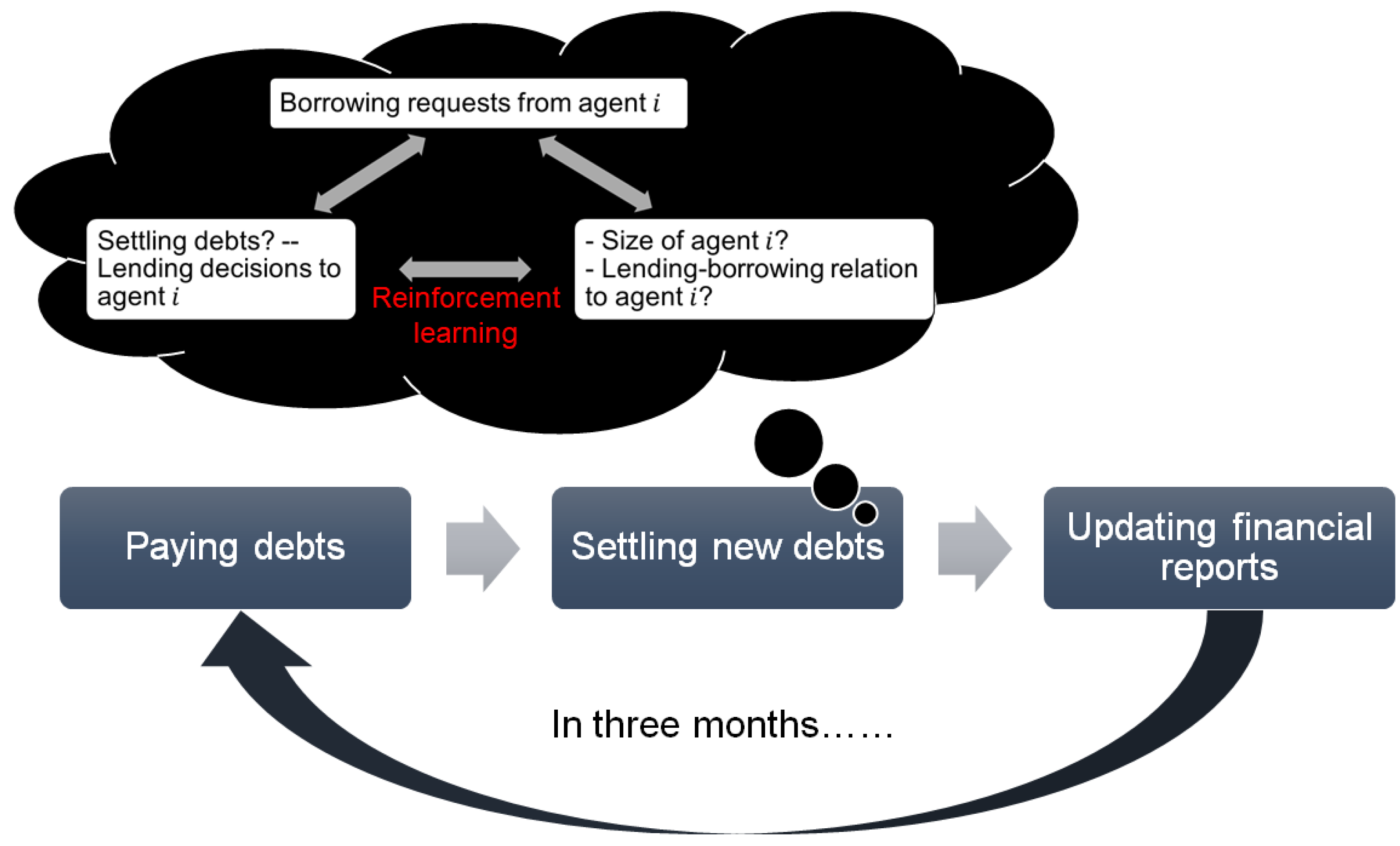
This section presents a multi-agent model to simulate the U.S. interbank lending market. Banks, or agents, are involved in an iterative dynamic framework. One iteration is equivalent to a quarter, or three months. In each iteration, agents finish three activities: paying debts, settling new debts, and updating financial reports (see Figure 1). Settling debts, the key of interbank market network dynamics emerging endogenously, involves a reinforcement learning process in which banks’ judgments and selections of counterparties evolve based on previous lending–borrowing decisions (see Figure 1).

This modeling framework builds the linkage between balance sheet changes and the interbank network structure shifts through banks’ interbank lending–borrowing decisions. It captures, through a long-term horizon, how lending–borrowing links among banks are established and how the interbank network is formed. Despite exploring individual banks or individual links, this framework captures the emerging interbank market properties from a system’s perspective.

3.1. Multi-Agent Interbank Market Framework

The model initializes a lending network with 6600 banks linked by interbank debts. There are two types of banks and three types of debts (see

Table 1. Interbank network setting.

Node Types: Banks’ size type is based on assets from 2001 to 2014, detailed approach is documented in [34]
Large Banks	Bank of America, Citibank, J.P. Morgan Chase Banks, and Wells Fargo Bank
Small Banks	Other Banks
Link Types:
Overnight debts	Federal funds, usually expire overnight
Short-term debts	Federal securities, usually expire within three months
Long-term debts	Loans expire less than one year

). The majority of interbank debts expire no more than one year as the purpose of this market is liquidity. Therefore, we only consider the loans and the amount borrowed expiring within one year on banks’ balance sheets. Among interbank transactions, federal funds and securities settled through Fedwire services are clearly stated as overnight and less than three-month debts, respectively. By the interbank market convention, other debts, expiring between three-months and one year, are recorded as long-term debts.

The interbank market is the environment in which banks incorporate with each other. Banks not only adopt information from the environment, but also reshape the interbank network through their routinized activities and decisions.

3.1.1. Paying Debts

In every iteration, banks first process payments to existing debts. According to expiration of the three types of interbank lending, overnight debts are paid fully, short-term debt payments and long-term debt payments are drawn from U(99%, 100%) and U(25%, 100%), respectively. We adopt the Eisenberg–Noe iterative clearing vector algorithm to clear payments [7]. In this process, banks may face liquidity or solvency issues that prevent them from fulfilling their obligations (see Equations (4) and (5)). In this case, the lenders realize write-down for debts with defaulting banks according to the Eisenberg–Noe algorithms pro rata loss distribution method.

3.1.2. Settling New Debts

Banks settle debts by actively searching for counterparties. Generally, as shown in Figure 1, each bank sends borrowing requests to potential lenders, and lenders respond with approval or rejection. In the model, banks first check their current balance sheet ratios and the target ratios to establish their demand of lending and borrowing in overnight, short-term, or long-term markets. For example, if a bank’s current overnight lending ratio is lower than its target, it will look for borrowers in the overnight market. Similarly, if a bank’s current overnight borrowing ratio is lower than its target, it will look for a lender in the overnight market. A bank will keep seeking counterparties until it reaches all of its targets.

Zooming into details of the acceptance of borrowers, a score-driven process is then applied to each borrowing request. Banks keep track of two scores for all other banks in order to pick the counterparties for new debts: a size score, $S^{\mathrm{size}}$, and a relationship score, $S^{\mathrm{relation}}$.

The size score is calibrated through the comparison of bank size to the average size of existing counterparties. This is consistent with the preference of banks to build interbank market relationships with large banks:

$$\begin{array}{cc}\hfill S_{i,j}^{\mathrm{size}}(t)& =log{A}_j(t)-{\displaystyle \frac{{\sum }_{k,k\ne i}log{A}_k(t-1){\mathbb{I}}_{i,k}(t-1)}{{\sum }_{k,k\ne i}{\mathbb{I}}_{i,k}(t-1)}},\hfill \\ \hfill {\mathbb{I}}_{i,k}(t)& =\{\begin{array}{c}1,\mathrm{if}i\mathrm{and}k\mathrm{are}\mathrm{connected}\mathrm{on}\mathrm{period}t,\hfill \\ 0,\mathrm{otherwise},\hfill \end{array}\hfill \end{array}$$

(1)

where $S_{i,j}^{\mathrm{size}}(t)$ is the size score of bank j evaluated by bank i on the period t, $A_j$ is the total assets of bank j, ${\mathbb{I}}_{i,k}(t)$ is a binary variable for keeping track previous debt obligations.

“Relationship” in this paper particularly denotes a interbank market lending–borrowing relationship. Other types of business cooperations are not considered or modeled. Therefore, the relationship score captures the willingness of two banks to become conterparties in the interbank market. The rationale of this score is to form the positive feedback loop between existing counterparties: the more debt between two banks, the higher $S^{\mathrm{relation}}$, and in return the more likelihood for new debt. As the lending–borrowing relations are determined endogenously through the iterative activities, banks quantifying $S^{\mathrm{relation}}$ of other banks in a dynamic process—the reinforcement learning—which will be introduced in Section 3.2.

Upon receiving a borrowing request, banks go through two key questions: (1) should they provide new debts to borrowers? (2) how much should be lent to each requester? Possessing lending preferences, each bank with space in its overnight, short-term, or long-term lending follows a similar scoring system as described in Equation (2). Accordingly, banks go through each request and make decisions until lending targets are completed or there are no more requests left to fill. However, banks may refuse to accept requests from other banks in the market even though they have capacity. The banks utilize an S-shaped function, $p(S_{i,j}^{\mathrm{total}})$, to assess the chance to lend to each specific borrower (see Equation (3)):

$$S_{i,j}^{\mathrm{total}}=\omega S_{i,j}^{\mathrm{relation}}+(1-\omega )S_{i,j}^{\mathrm{size}},$$

(2)

where $s(i,j)$ is the score that borrower i assigns to lender j. It is the weighted average of relationship score and size score of bank j. We set equal weights to these scores so that $\omega =0.5$:

$$p(S_{i,j}^{\mathrm{total}})={\displaystyle \frac{1}{1+exp(\alpha +\beta \times S_{i,j}^{\mathrm{total}})}}.$$

(3)

The use of an S-shaped function is inspired by the “logistic classifier”. It is widely applied in modeling choices between two alternatives. In our model, banks determine whether to lend out their excess liquidity, which is also a binary decision scenario. The S-shaped function stems from the standard logistic function. Moreover, this setting allows us to investigate the impact of risk preference. In this function, $p(S_{i,j}^{\mathrm{total}})$ presents the probability that borrower i lends to lender j, and $\alpha$ and $\beta$, respectively, control intercept and slope. $\alpha$ is a real number, and represents the risk preference level of a bank. The larger the $\alpha$, the more chance to lend to a low scored counterparty. This insight has also been described by [34].

Following a uniform distribution, lending banks decide the fraction they want to lend out from their lending pool. The new debt amount is set as the lower value between the one determined by the lending bank and requested by the borrowing bank. This new debt established is observed by both banks as a reward that their bank balance ratios are moving closer to their respective target ratio.

3.1.3. Updating Financial Reports

At the end of each iteration, banks process balance sheet updates to realize collected payments and latest borrowing/lending activities. Moreover, we incorporate retained earnings based on an empirically fitted distribution Beta(17.36, −0.1, 0.3):

$$E_i(t)<A_i(t)-L_i(t),$$

(4)

where $E_i(t)$, $A_i(t)$, and $L_i(t)$ are bank i’s equity, asset, and liability on period t:

$$C_i(t)<{ON}_i^p(t)+{ST}_i^p(t)+{LT}_i^p(t),$$

(5)

where $C_i(t)$, ${ON}_i^p(t)$, ${ST}_i^p(t)$, and ${LT}_i^p(t)$ are bank i’s cash and cash equivalents, payments of overnight borrowing, payments of short-term borrowing, and payments of long-term borrowing on period t.

3.2. Bank Lending-Borrowing with Reinforcement Learning

The reinforcement learning guides bank decisions of lending and borrowing (see Figure 1). More specifically, it leads the calibration of $S^{\mathrm{relation}}$ applied in the“settling new debts” activity (see Section 3.1.2). The key reason for applying a learning approach is to overcome the difficulties in reproducing bilateral lending–borrowing relationships through balance sheet data. Existing analytical solutions to the bilateral exposure problem largely rely on some sort of optimization scheme that produces unrealistic results [34,35]. Knowing that these solutions cannot be improved to produce a more realistic model, we allow the agents to reorganize their lending–borrowing decisions to form bilateral links naturally through the reinforcement learning.

In this multi-agent simulation, reinforcement learning is involved in both model initialization and agents’ iterative decisions. This learning process plays a critical role in the model convergence. The interbank network is initially formed by a maximum entropy approach, which generates too many links compared with empirical findings of the real U.S. overnight interbank market. Hence, banks reform links through reinforcement learning until they reach a new stabilized network. In this process, interbank transactions and bank failures do not occur. The initialization ends with the convergence of average temporal difference in learning. Then, interbank market transactions, debt payments, and balance sheet updates start from this time point, and learning continues to fine-tune banks’ decisions and generate minor network changes.

The rest of this section discusses the reinforcement learning process, and how banks approach $S^{\mathrm{relation}}$ of other banks based on this process. Reinforcement learning is a computational technique that allows agents to learn and determine the ideal behavior based on past experience. Similar to the agent-based simulation, reinforcement learning is also an iterative process that allows us to embed it fully into the multi-agent interbank system. There are three elements that drive the interaction between an agent and the environment: state, action, and reward. A state s refers to all current information in the environment received by an agent. Each agent then follows the policy $\pi$ to map the state s to an action a (i.e., $\pi :s\to a$). The action may cause changes in state, and, more importantly, provide feedback to the agent with rewards. The rewards lead agents to converge their evaluation of $S^{\mathrm{relation}}$ among others.

3.2.1. Banking System States

In the multi-agent system, public information available to agents are banks’ size and existing lending–borrowing relations. We use two scores to quantify the states: $S^{\mathrm{size}}$ (see Equation (1)) and $S^{\mathrm{relation}}$. The relationship score captures the preference of continuing business with existing counterparties. It is updated upon receiving the reinforcement signal from the lending and borrowing actions a bank makes in each iteration. In the model, the temporal difference (TD) method is adopted to update the relationship score (see Section 3.2.3). In addition, banks also hold private information about their own target ratios and evaluate the status of their balance sheet to help guide the lending and borrowing policy. We assume that each bank has a settled business model that determines the fraction of assets (or debts) to lend (or borrow) in overnight, short-term, and long-term markets.

3.2.2. Actions—Bank’s Lending and Borrowing Decisions

Banks are modeled as passive learning agents that rely on a fixed policy to select their lending and borrowing counterparties. However, agents may learn to select better counterparites by learning and updating the $S^{\mathrm{relation}}$.

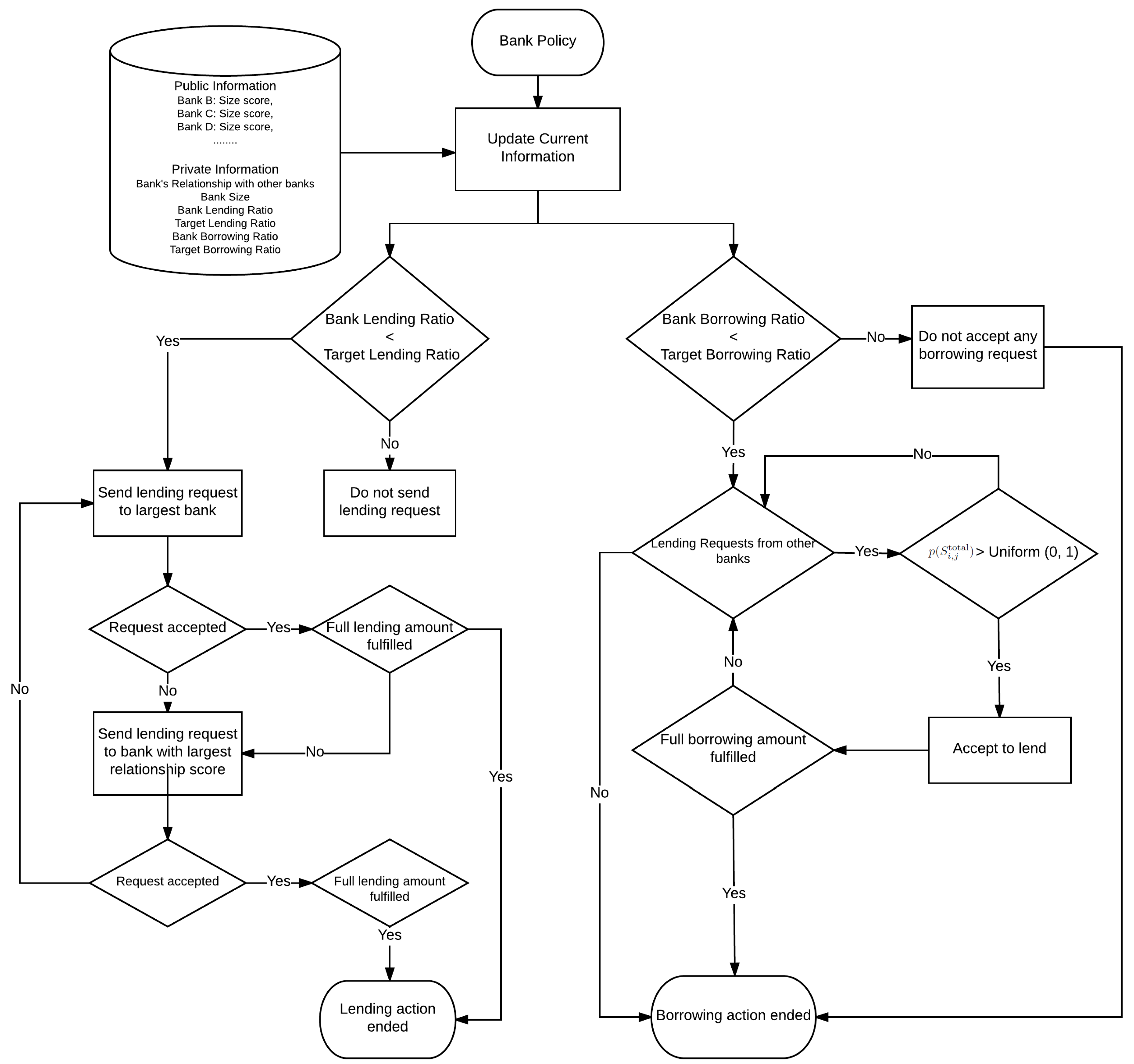
Banks’ lending and borrowing needs are determined by target ratios. Targeting borrowing expectations, first each bank would send borrowing requests to large banks based on $S^{\mathrm{relation}}$ because of greater opportunities to obtain funds. As long as the targets are not met entirely, it sends requests to the highest scoring bank. If the targets are still not completed, it goes to the highest $S^{\mathrm{size}}$ bank and asks for new debts. This process would continue until the requests are satisfied perfectly or no more funds are available in the market. The lending policy, as illustrated in Section 3.2, is derived from an S-shape function. In summary, the flow of the bank’s policy can be represented and illustrated by Figure 2.

3.2.3. Temporal Difference Learning Update

The TD algorithm combines the characteristics of both the Monte Carlo method and dynamic programming. Similar to the Monte Carlo method, the TD algorithm is a model-free approach that is able to evaluate the value of a given state by learning directly from past experiences. In addition, it also incorporates the idea of bootstrapping from dynamic programming that the estimation of their update is based on a previous estimate. In this model, we use the $TD(0)$ method to allow banks to learn from past lending and borrowing actions. $TD(0)$ is formulated as follows:

$$V(s_t)=V(s_t)+\varphi [r_{t+1}+\gamma V(s_{t+1})-V(s_t)],$$

(6)

where $V(s_t)$ is the estimate of expected sum of discounted rewards at time t, $r_{t+1}$ denotes the observed reward, $\varphi$ is the learning rate, and $\gamma$ is a discount factor for $V(s_{t+1})$.

In the model, at the beginning of each iteration (a quarter), each bank determines its lending and borrowing actions according to the bank policy described in the previous section. Lending and borrowing actions are decided by the size score of each bank and relationship score between two banks. Since size score is determined by the total assets presented in the balance sheet, banks do not update the size score using the temporal difference method. However, since the nature of the relationship score is to capture a bank’s tendency to keep existing relationships, banks update their relationship score with other banks by using the $TD(0)$ algorithm. The updating process is described below.

When bank i and bank j established a new relationship, the relationship score between the two banks, $S_{i,j}^{\mathrm{relation}}$, will be updated using Equation (6). At the beginning of each quarter, TD learning is applied to every bank to update their relationship score. In Equation (6), $V_t$ denotes the bank’s evaluation of its relationship score with all other banks. $V_{t+1}$ is the estimation of the sum of debts established in the future and it can be formulated as Equation (7). In this model, banks assume that all debts received from that counterparty are equal to the last reward observed in the future. Therefore, Equation (7) can be expended and simplified to Equation (8):

$$V(s_{t+1})={\displaystyle \sum _{k=0}^{\infty }}{\gamma }^k\times r_{t+k+2},$$

(7)

$$\begin{array}{cc}\hfill V(s_{t+1})& ={\displaystyle \sum _{k=0}^{\infty }}{\gamma }^k\times D_{t+k+2}\hfill \\ & =(\gamma \times D_{t+2})+(\gamma \times D_{t+3})+(\gamma \times D_{t+4})+\dots \hfill \\ & =D_{t+1}(1+{\gamma }^1+{\gamma }^2+\dots )\hfill \\ & ={\displaystyle \frac{D_{t+1}}{(1-\gamma )}},\hfill \end{array}$$

(8)

where $D_t$ is the new debt between two banks in period t.

As a result, the $TD(0)$ updating process of relationship score can be expressed as:

$$S_{i,j}^{\mathrm{relation}}(t)=S_{i,j}^{\mathrm{relation}}(t)+\varphi [D_{t+1}+\gamma {\displaystyle \frac{D_{t+1}}{(1-\gamma )}}-S_{i,j}^{\mathrm{relation}}(t)].$$

(9)

We make a further assumption that the learning rate $\varphi$ is equal to $1-\gamma$, resulting in:

$$\begin{array}{cc}\hfill S_{i,j}^{\mathrm{relation}}(t)& =S_{i,j}^{\mathrm{relation}}(t)+\varphi [D_{t+1}+{\displaystyle \frac{(1-\varphi )}{\varphi }}{D}_{t+1}-S_{i,j}^{\mathrm{relation}}(t)]\hfill \\ & =S_{i,j}^{\mathrm{relation}}(t)+D_{t+1}-\varphi S_{i,j}^{\mathrm{relation}}(t)\hfill \\ & =(1-\varphi )S_{i,j}^{\mathrm{relation}}(t)+D_{t+1}.\hfill \end{array}$$

(10)

4. Data

Financial reports are one of the key information sources that disclose banks’ financial fundamentals and business conditions. The Federal Reserve, the FDIC, and the Office of the Comptroller of the Currency (OCC) require all U.S. regulated banks to submit quarterly reports known as Federal Financial Institutions Examination Council (FFIEC) Reports of Condition and Income. Those banks include national banks, state member banks and insured state nonmember banks. Similar to regulators that rely on balance sheets to monitor banks’ liquidity status and banking system structures, we use balance sheets data from March 2001 to December 2014, covering around 10,000 banks (see

Table 2. Description of the bank balance sheet.

Asset: A	Liability: L
Overnight lending: $O{N}^l$	Overnight borrowing: $O{N}^b$
Short-term lending: $S{T}^l$	Short-term lending: $S{T}^b$
Long-term lending: $L{T}^l$	Long-term borrowing: $L{T}^b$
Cash and balance due: C	Other liabilities: OL
Other assets: OA	Equity: E

).

In the model, we assume that banks target a series of balance sheet ratios (see

Table 3. Banks’ target ratios.

Equity Multiplier	E/A
Overnight lending, borrowing ratio	$(O{N}^l/A)$ , $(O{N}^b/L)$
Short-term lending, borrowing ratio	$(S{T}^l/A)$ , $(S{T}^b/L)$
Long-term lending, borrowing ratio	$(L{T}^l/A)$ , $(L{T}^b/L)$

), associated with banks’ decisions of lending and borrowing. These targets guarantee that banks maintain their lending–borrowing preferences for overnight, short-term, and long-term debt. Additionally, we use the equity multiplier, the ratio of its total assets to its equity, to control a bank’s expected leverage. Even though banks do not explicitly optimize their decisions to reach these ratios, empirical data show that these targets are driven by the banks’ business model implicitly and are robust over a long time horizon [34].

We model and validate the pre-crisis interbank network in this study, using data before 2006 to calibrate the ratios. Indeed, we observed banks changing target ratios post-crisis due to new policies and the economic situation [34]. The potential network structure changes based on new target ratios are not discussed in the scope of this study. We may explore in the future work.

Banks are not guaranteed to reach their targets every quarter through the lending–borrowing process. This will not affect the banks’ decision-making policies, but it may lead to liquidity risk. An extreme case is that if a bank keeps ending up with failed borrowing requests, it will get into a situation of low cash and cash equivalents. If this causes distress to its ability of paying existing debts, the bank will fail due to liquidity issues.

5. Model Validation

We run a number of validation exercises to ensure that the model can produce inter-bank markets resembling the real interbank markets. We use the data of 6600 banks that had been operating before 2006. Banks hold varied assets from 3000 to 1.5 billion. The agents’ target ratios and initial balance sheets are calibrated by the average value through 2001 to 2006 (see

Table 4. Data summary of target ratios.

	Min.	Median	Mean	Max.
$O{N}^l/A$	0.00%	1.29%	2.49%	94.82%
$O{N}^l/L$	0.00%	0.00%	0.55%	84.11%
$S{T}^l/A$	0.00%	0.00%	0.23%	36.18%
$S{T}^b/L$	0.00%	0.66%	2.15%	41.99%
$L{T}^l/A$	0.00%	0.00%	0.25%	76.43%
$L{T}^b/L$	0.00%	0.15%	1.11%	81.79%
$E/A$	4.20%	9.20%	11.38%	99.24%

).

Table 5. Summary of parameters.

Parameter	Value
$\alpha$	Large banks −1.0; small banks 0.0
$\beta$	1.0
$\omega$	0.5
$\varphi$	0.5

lists parameters used in this model. $\varphi$ only controls the reinforcement learning converging speed and stability. We set a value that gives reasonable converging pattern (see Section 5.1). As there is no literature showing whether banks have priority in size or the relationship to make lending–borrowing decisions, we set $\omega =0.5$, indicating equal weights to these factors. $\alpha$ and $\beta$ are particularly tuned to match network properties in Section 5.2 and different risk preferences of large and small banks. We found that the change of $\beta$ does not affect the network structure much. A more comprehensive discussion of sensitivity to the risk preference parameter $\alpha$ is in Section 6.2.

5.1. Convergence of Relationship Score Learning

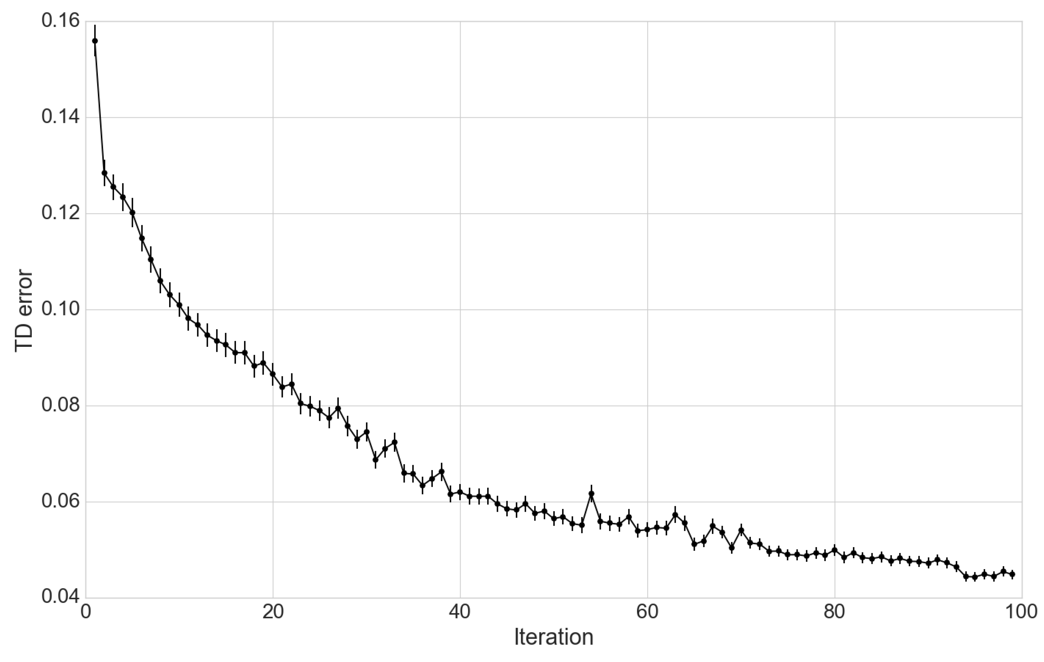
In the model initialization, banks use temporal difference learning to update their relationship scores as they receive reinforcement signals from borrowing and lending actions. In this experiment, we study the effectiveness of applying the $TD(0)$ method in a complex interbank network environment. Ref. [33] provides thorough proof that the $TD(0)$ method converges to a optimal evaluation for linear problems. However, the effectiveness of applying the $TD(0)$ method in complex real-world problems remains unclear. Ref. [36] investigates the effectiveness of the TD method on complex practical issues such as the game of backgammon and self-play. In this model, we validate the use of temporal difference learning by investigating the convergence of relationship score (the TD updating target) over time.

The experiment runs for 100 iterations of bank lending and borrowing interactions. At each iteration, the mean squared error of relationship score is recorded and computed for the entire bank population. From Figure 3, we can see that the mean squared error of the relationship score converges as the system runs for 100 iterations.

5.2. Network Properties Validation

We validate the overnight lending market with the U.S. federal fund market. Ref. [37] collected interbank transactions in 2006 from Fedwire and analyzed the empirical network topology. The network is a directed network with links from lender to borrower, and we verified the following three measures:

• Degree: For each node in a network, the number of links directing to the node is called its in-degree, and the number of links directing out from the node is its out-degree. Average values are taken to measure the degree from the network-based perspective. As the “zero degree” nodes are not counted in the average, in-degree and out-degree values are different.
• Clustering coefficient: It is a closeness measure. A node’s clustering coefficient is the number of links between the node within its neighbors divided by the total number of links that could be formed between them. The in-clustering counts the links to the node, and the out-clustering counts the links from the node. Similar to network degree measures, network in-clustering and out-clustering are also average values across all nodes.
• Power law: A power law distribution is defined as $P(k)\sim k^{-\gamma }$. In network analysis, “power law” parameter $\gamma$ is calibrated by fitting the degree histogram to the power law distribution. A detailed calibration methodology is introduced by [38]. In this paper, we regard the network as an indirected network when calibrating the power law.

To compare the network structures, we conducted 100 experiments with the same number of agents (see

Table 6. U.S. Federal funds market interbank network property comparison (100 simulations).

	Average In-Degree	Average Out-Degree	Average In-Clustering	Average Out-Clustering	Power Law
U.S. Fed. Funds Market	9.30	19.10	0.10	0.28	2.00
Model	10.51	17.17	0.03	0.31	2.00
	(0.14)	(0.09)	(0.00)	(0.02)	(0.00)

Notes: This table lists the key network measures between the real U.S. federal funds market and the simulation results. For the In-Degree and Out-Degree measure, we used the GSCCD—giant strongly connected component reported in [37] for the reason that it reflects the interbank market mostly. For the model results, we show standard deviation in parentheses below the reported average results. Source: [37]: Authors’ calculations.

). An interesting finding is that the intelligent agents generate a network structure that is very close to our previous study [34].

6. Experiments and Discussion

The multi-agent learning model simulates the banking system dynamics and provides a realistic tool to investigate problematic issues in the interbank lending system. In this section, we conduct two experiments to examine the model effects on interbank market structures due to banks’ risk behaviors.

6.1. Interbank Network Topologies

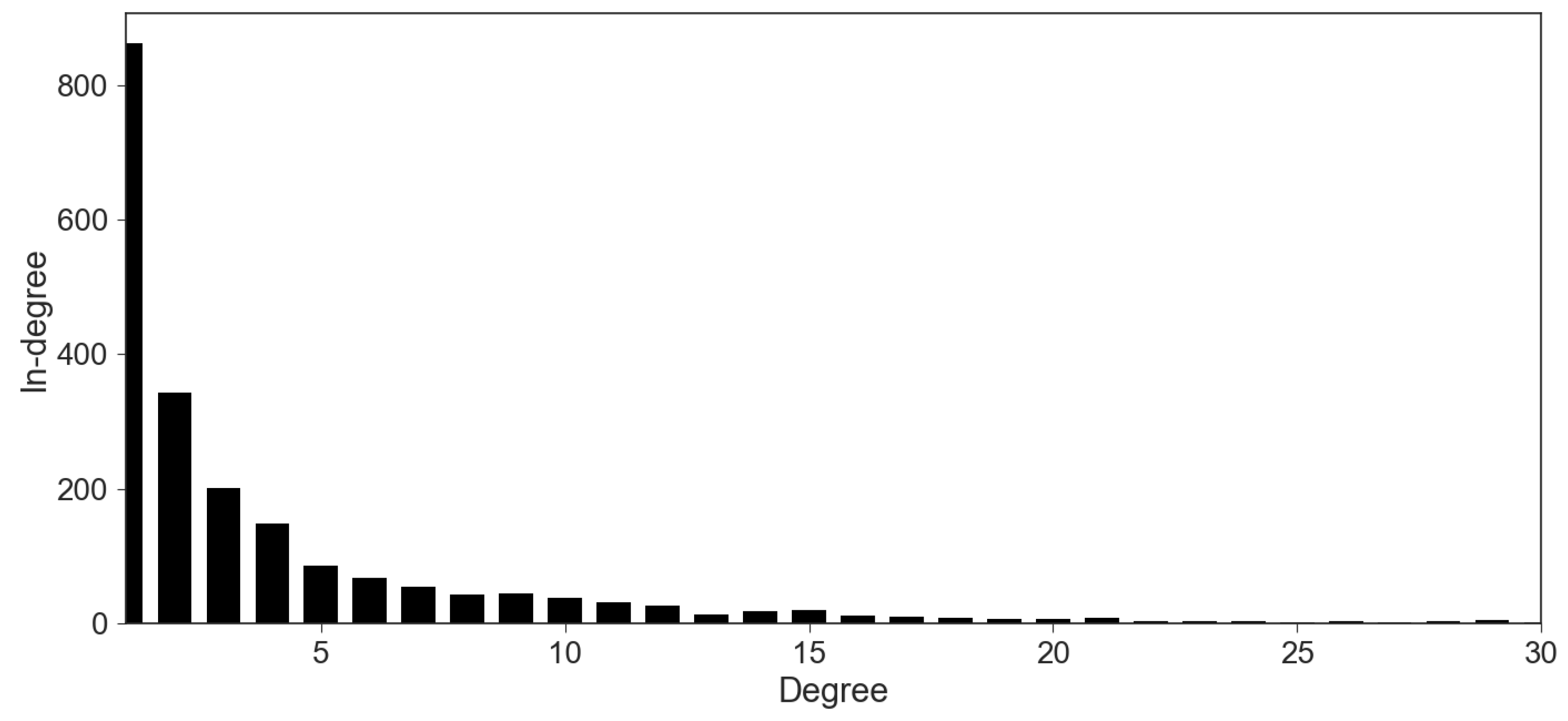
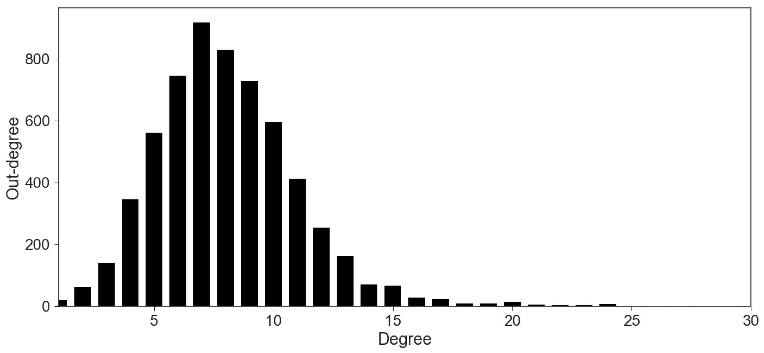
Interbank network degree is asymmetric. Both in-degree and out-degree are heavily rightly skewed, indicating that most bank agents have few established relationships (see Figure 4 and Figure 5). Moreover, we observe a power-law decaying pattern in the in-degree distribution (see Figure 4). Obviously, banks prefer to maintain a lower number of lenders. Over 10% of banks only borrow from one lender. However, it is not common to minimize the number of borrowers due to consideration of risk diversification. Even though we do not have real interbank market transaction data to compare the results, we can confirm the stylized facts documented in [24].

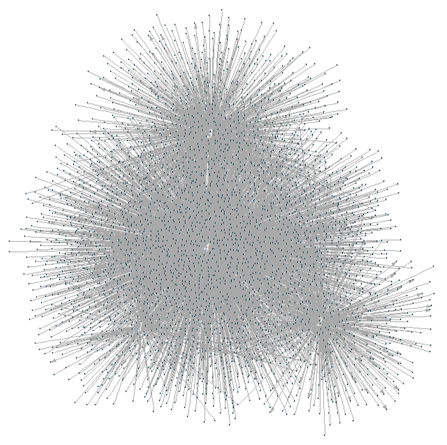
In this experiment, we examine the interbank network structure after 50 iterations of the model simulation and discuss the preliminary results that show the differences between a risk-seeking lending policy and a risk-averse lending policy. We present two network structures that identify the lending and borrowing relationships between banks. Figure 6 shows the interbank network when banks adopt a risk-seeking lending policy and Figure 7 shows the network when banks become more risk averse in accepting lending requests. In both network plots, we labeled the four large bank agents as “1, 2, 3, 4” because empirical studies have suggested that they tend to establish more lending and borrowing relationships than other banks [24]. From these results, we discover that large banks tend to form their own clusters when they employ a risk seeking policy. On the other hand, this phenomenon becomes less obvious when they adopt a more risk-averse policy.

6.2. Network Adaptation and Risk Preferences

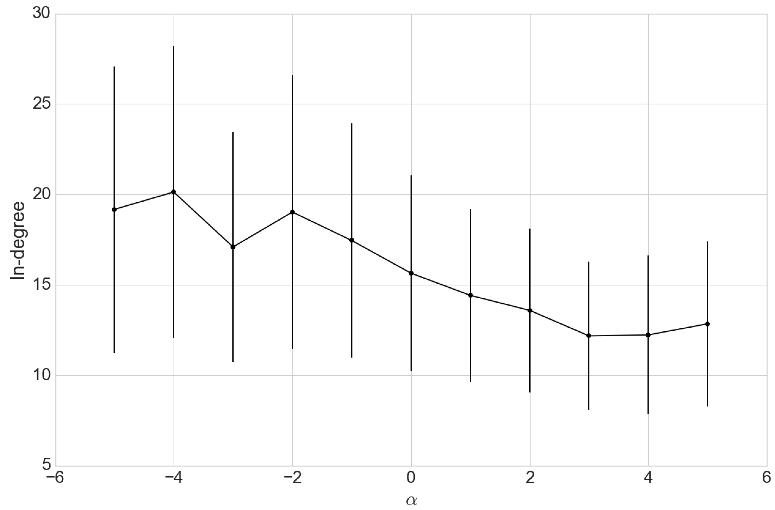
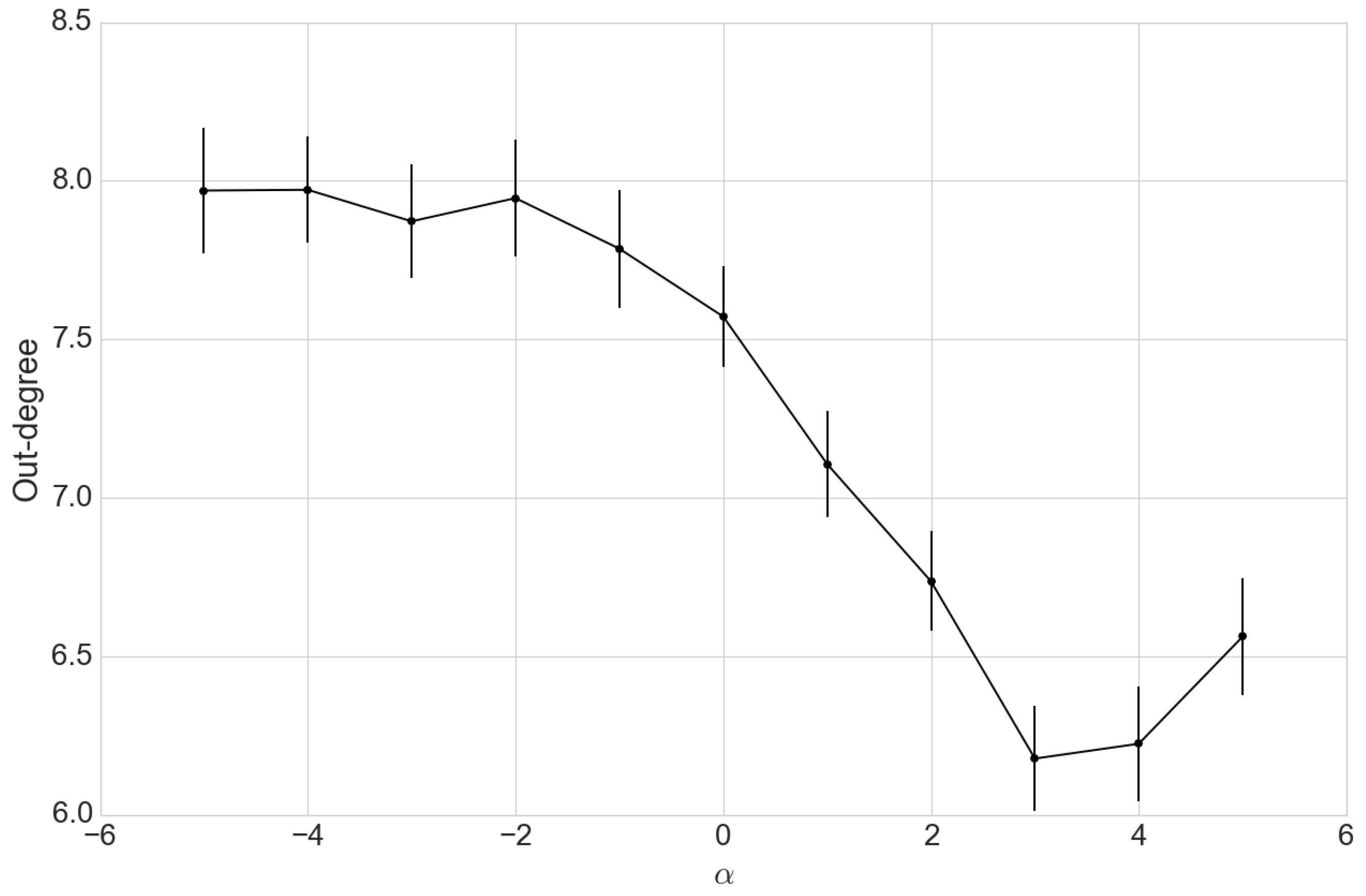
The bank lending policy (Equation (3)) shows that $\alpha$ is the risk tolerance parameter. A small $\alpha$ represents higher risk tolerance. Putting differently, when $\alpha$ decreases, banks adopt a risk-seeking lending policy and have a higher chance to lend out. In this experiment, we study the network property adaptation by altering $\alpha$ from −5 to 5. We explore changes in average degree, clustering coefficient, and average shortest path (see

Table 7. Interbank network properties.

Overnight	Average Degree	Clustering Coefficient	Power Law	Average Path
Risk-Seeking Policy	15.12	0.35	2.39	2.34
Risk-Averse Policy	11.51	0.19	2.42	2.66
Short-term	Average Degree	Clustering Coefficient	Power Law	Average Path
Risk-Seeking Policy	1.04	0.43	2.44	2.30
Risk-Averse Policy	1.04	0.53	2.29	2.21
Long-term	Average Degree	Clustering Coefficient	Power Law	Average Path
Risk-Seeking Policy	2.42	0.40	2.14	2.44
Risk-Averse Policy	2.42	0.57	2.15	2.28

). These network characteristics of the interbank systems are generally in line with the empirical observations [11,22,23].

As the model forms a directed network in which edges are pointing from lender to borrower, we can measure how the calibration of $\alpha$ impacts the average number of in-degree (lending) and out-degree (borrowing) relationships. We observe similar patterns for the two measures. The network degree is stable when $\alpha <-1$; however, the degree decreases with increasing $\alpha$ (see Figure 8 and Figure 9). This result confirms that a tightened lending policy reduces the amount of debt, or counterparities, in interbank networks. Moreover, the 95% confidence interval of in-degree is much larger than that of out-degree. These results are consistent with our findings of asymmetric distributions for lending and borrowing. With an increasing $\alpha$, it becomes harder for banks to find lenders such that the in-degree is decreasing with a tighter confidence interval (see Figure 8).

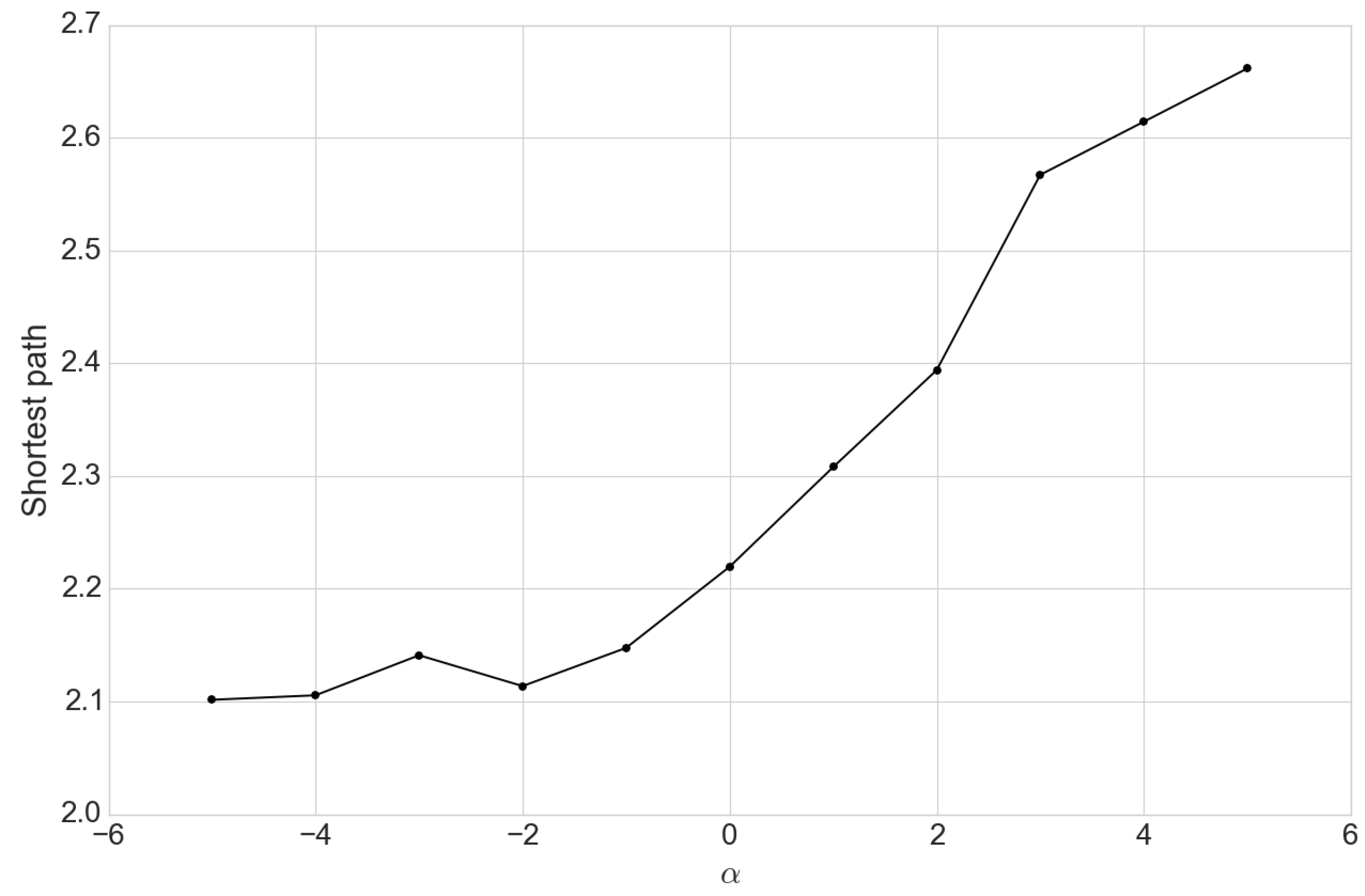
The average network shortest path, as shown in Figure 10, agrees with the hypothesis that interconnectedness of banks declines as $\alpha$ increases. We observe a longer distance among banks when $\alpha$ is positive, indicating that the whole system is less connected.

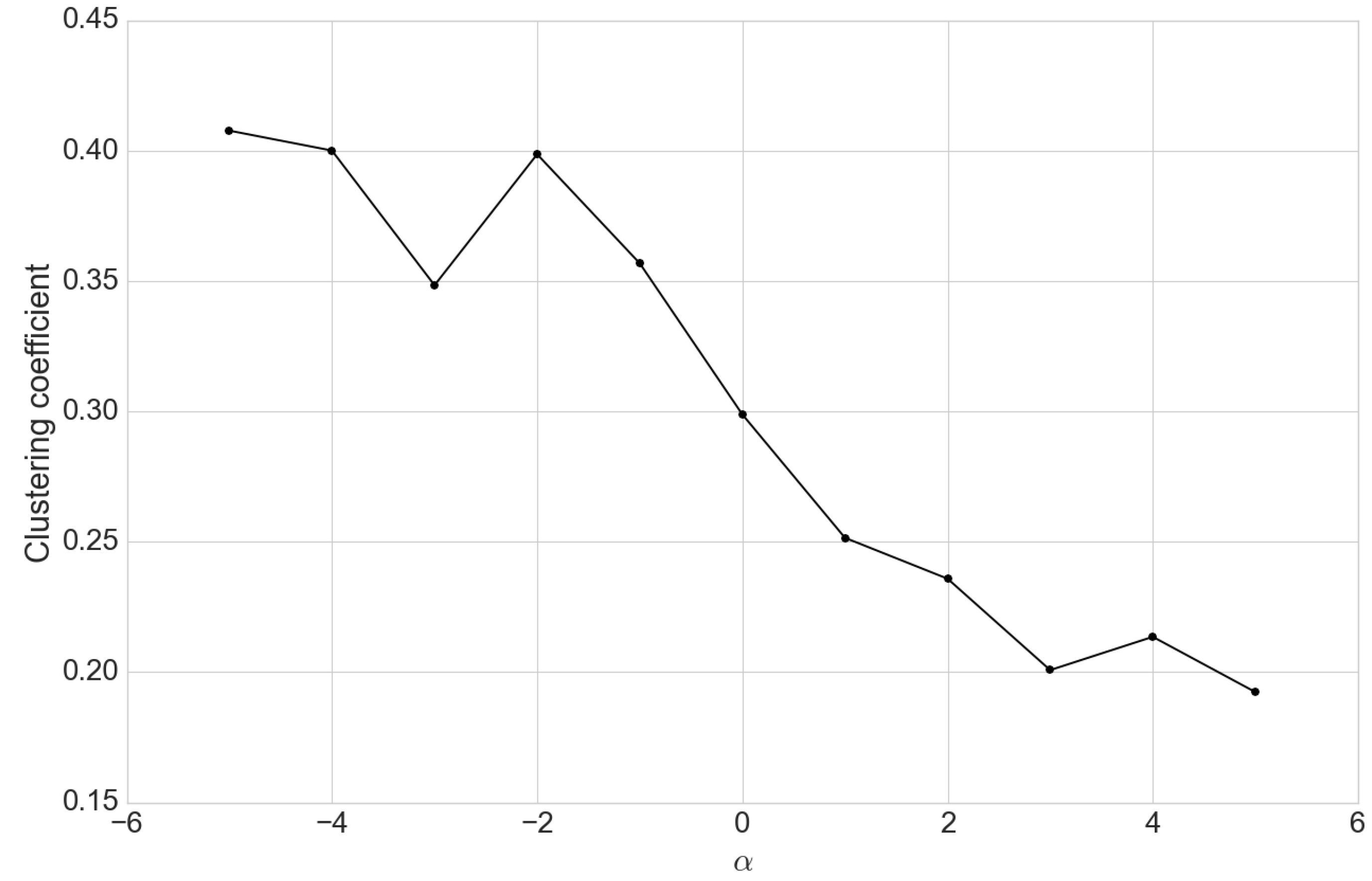
Upon inspecting Figure 11, we find that the clustering coefficient of the network becomes less clustered as the risk aversion increases. This phenomenon shows that, when banks become more averse to lending to other banks, the network becomes less clustered, thus more sparse than complete. This is validated by also a decreased degree and increasing average shortest path, which also indicate a loosely connected network.

7. Conclusions

This study proposes a multi-agent learning model to reconstruct interbank lending networks and examine their dynamics. We incorporate a reinforcement learning framework to guide bank decisions. Banks learn and update their choice parameters based on past interaction within the system. Our model is able to capture the individual preferences of banks while allowing them to vary their policies to the environmental conditions presented.

Two experiments are conducted in this study to investigate the network properties of the interbank lending market as adaptive bank risk preferences are varied. First, we look at two different interbank networks of banks adopting a risk-seeking lending policy and a tightened lending policy, respectively. We compare the network properties of the two interbank lending networks, and show that, given a certain level of risk preference, the network degree begins to decline as banks continue to tighten their lending policies. Secondly, we examine the interconnectedness of bank agents by computing the clustering coefficients and average shortest path amount banks. This suggests that, as banks tighten their lending policies, the network becomes sparser and thus more concentrated. As a result, the interbank network is less at risk for concerns of contagion. Though banks are less likely to find new counterparties, they are generally more capable of sustaining stresses, thus demonstrating how individual choices present beneficial overall market structure condition due to the adaptive learning capabilities of the banks. This finding supports the general observation during the financial crisis.

The methodology proposed in this study offers a new perspective on how one can utilize reinforcement learning to model bank agents. Combined with the use of financial data, we provide guidance on how central banks and regulators may consider building more functional models for examining the interbank systemic risks. Future research might include exploring how banks dynamically select the optimal policy based on the observed states, and consider how monetary policy influences competition in interbank lending.

References