A Green Supplier Assessment Method for Manufacturing Enterprises Based on Rough ANP and Evidence Theory

Abstract

Within the context of increasingly serious global environmental problems, green supplier assessment has become one of the key links in modern green supply chain management. In the actual work of green supplier assessment, the information of potential suppliers is often ambiguous or even absent, and there are interrelationships and feedback-like effects among assessment indexes. Additionally, the thinking of experts in index importance judgment is always ambiguous and subjective. To handle the uncertainty and incompleteness in green supplier assessment, we propose a green supplier assessment method based on rough ANP and evidence theory. The uncertain index value is processed by membership degree. Trapezoidal fuzzy number is adopted to express experts’ judgment on the relative importance of the indexes, and rough boundary interval is used to integrate the judgment opinions of multiple experts. The ANP structure is built to deal with the interrelationship and feedback-like effects among indexes. Then, the index weight is calculated by ANP method. Finally, the green suppliers are assessed by a trust interval, based on evidence theory. The feasibility and effectiveness of the proposed method is verified by an application of a bearing cage supplier assessment.

1. Introduction

With the increasing awareness of global environmental protection and the increasing number of related environmental regulations, manufacturing enterprises are facing more stringent environmental requirements. Nowadays, green supply chains have become inevitable choices for manufacturing enterprises who wish to deal with environmental problems. Green supply chain management includes many links, such as green supplier assessment, green product design, green production, green marketing and waste recovery [1,2,3]. Green supplier assessment is in the upstream of the whole supply chain, and its effect on environmental protection and cost saving can be transmitted to every part of the downstream through the supply chain.

In the process of green supply chain management, various factors make the relationship between suppliers and manufacturing enterprises complicated and vague. However, competitors constantly adjust their strategies, and the supply chain must constantly improve to adapt to the complex environment which changes rapidly. In this context, green supplier assessment plays a very important role in reducing costs, and improving product quality and market competitiveness. Through effective assessment and supervisions of suppliers, problems can be found and solved in time, and the green and healthy development of the entire supply chain can be promoted [4,5,6,7,8,9]. It can be seen that green supplier assessment plays a decisive role in green supply chain management, which directly determines the competitiveness of the entire supply chain. The rise of the internet has provided convenience for manufacturing enterprises to assess green suppliers, but enterprises cannot quickly choose suppliers which meet their needs in the face of so many uneven suppliers. Considering finances and the effective utilization of resources, how to assess green supplier quickly and effectively becomes the key problem in modern green supply chain.

As seen in the present literature, there are many significant works on green supplier assessment. On the whole, the existing research mainly includes the following aspects.

(1)

Supplier assessment models based on Analytic Hierarchy Process (AHP) [10] or Analytic Network Process (ANP) [11]. Noci [12] used AHP to evaluate supplier’s environmental efficiency. Lee et al. [13] used the Delphi technique to distinguish the evaluation criterion difference between the traditional supplier and the green supplier, and then used Fuzzy Analytic Hierarchy Process (FAHP) to solve the green supplier selection process. Hsu and Hu [14] contained the interdependence between components of decision structure and used ANP for green supplier selection which reflected a more realistic result.

(2)

Supplier assessment model based on mathematical Programming. Yeh and Chuang [15] put forward a mathematical programming model of green partner selection, which includes four goals: cost, time, product quality, and green score. They adopted two multi-objective genetic algorithms (MOGA) to find a set of Pareto optimal solutions, and used weighted summation to generate more solutions. Yousefi et al. [16] used Dynamic Data Envelopment Analysis (D-DEA) and scenario-based robust model for supplier selection. In this supplier selection model, the shortcomings of the DEA model (the benchmarks were determined based on previous performance) were overcome, and the disadvantages of the D-DEA model (the decision unit couldn’t get a unified efficiency score) were avoided.

(3)

Supplier assessment model based on Technique for Order Preference by Similarity to an Ideal Solution (TOPSIS). Awasthi et al. [17] proposed a three-step method for green supplier evaluation: identification standard, expert score, evaluate expert score by fuzzy TOPSIS. The fuzzy TOPSIS method integrated profit and cost standard, and this method is suitable for the situation of lack of partial quantitative information. Kannan and Jabbour [18] used fuzzy TOPSIS to solve the problem of green supplier selection, and applies three types of fuzzy TOPSIS method to sort green suppliers.

(4)

Other hybrid models for supplier assessment. Gandhi et al. [5] proposed a combined approach using AHP and Decision-Making and Trial Evaluation Laboratory (DEMATEL) for evaluating success factors in implementation of green supply chain management and gave a case study in Indian manufacturing industries. Chatterjee et al. [19] combined DEMATEL and ANP in a rough context, and then proposed a rough DEMATEL-ANP (R’AMATEL) method to evaluate the performance of suppliers for green supply chain implementation in electronics industry. Wu et al. [20] used the Continuous Ordered Weighted Averaging (COWA) operator to transform the trapezoid fuzzy number into the exact real number to select the green supplier, and make a sensitivity analysis according to the degree of risk of decision-maker to rank the suppliers. Luo and Peng [21] proposed a multi-level supplier evaluation and selection model. In this model, AHP is used to determine the weights, and then TOPSIS is used for supplier evaluation. Kuo and Lin [22] integrated ANP and DEA and proposed a green supplier evaluation method. The interdependence between standards were considered by ANP, which allowed users to choose their own weight preferences to limit weights, expanded DEA method, and allowed more flexible number of decision units. Shi et al. [23] used the improved attribute reduction algorithm based on rough set to reduce the index of the green supplier evaluation index system, and then evaluated the data by RBF neural network training. Akman [24] identified the suppliers that should be included in the green supplier development plan through the C mean clustering algorithm and the VIKOR method. This method can be used to solve the problem of supplier classification and evaluation.

The study of green supplier assessment, which is of great theoretical and practical significance, has been a hot topic all along. However, the existing research has obvious shortcomings and the research gaps are mainly as follows:

(1)

The information of the suppliers to be assessed is not clear enough in the actual work of green supplier assessment. There is often no information sharing between manufacturing enterprise and suppliers, and the information between them is often ambiguous or even absent. The deterministic assessing model can no longer meet the needs of the increasingly complex decision-making environment.

(2)

Green supplier assessment is a complex decision problem and its indexes are interrelated. When calculating the index weight, the core idea of traditional AHP is to divide the index system into isolated and hierarchical levels. Only the upper level elements’ dominating effect on the lower level elements is considered and the elements in the same level are deemed to be independent of each other. However, the relationships among the indexes are often interdependent and sometimes provide feedback-like effects in green supplier assessment. Therefore, traditional AHP cannot solve the complex relationships among indexes to obtain the weight in green supplier assessment.

(3)

The accurate number is used to describe the relative importance of the indexes in the expression of experts’ judgment in most of the existing research, which cannot reflect the ambiguities and subjectivity of the actual thinking. It is more reasonable to use fuzzy numbers [25] to express the experts’ judgment. After introducing fuzzy numbers to express experts’ judgment, analyzing and processing the imprecise and inconsistent information becomes a difficult problem.

To fill the research gaps in green supplier assessment, a green supplier assessment method for manufacturing enterprises based on rough ANP and evidence theory is proposed. We process the uncertain index value by membership degree, adopt trapezoidal fuzzy number to express experts’ judgment on the relative importance of the indexes, use rough boundary interval to integrate the judgment opinions of multiple experts, set up the ANP structure to deal with the interrelationship and the feedback-like effects among indexes and then calculate the index weight by ANP method, and finally solve the incomplete information problem by evidence theory and assess the green suppliers by trust interval.

The rest of this paper is organized as follows. Section 2 establishes the index system of green supplier assessment; Section 3 uses membership degree method to process the uncertain index value of suppliers to be assessed; Section 4 adopts rough ANP to calculate the index weight; Section 5 gives the green supplier assessment procedure based on evidence theory; Section 6 provides an application case of bearing cage supplier assessment and discusses the feasibility and effectiveness of the proposed method for green supplier assessment. We conclude this paper in Section 7.

2. Index System

The first and very important segment of green supplier assessment is the establishment of a complete and overall index system. The attribute of the supplier’s product is the main representative of its ability, and the comprehensive ability of supplier can provide a strong support to its product. The comprehensive ability of supplier mainly includes internal competitiveness, external competitiveness and cooperation ability. Internal competitiveness of a supplier can be subdivided into its innovation capacity, manufacturing capacity and agility capacity. Furthermore, a supplier is not isolated and is inevitably restricted by its external competitiveness. External competitiveness of a supplier mainly includes its economic environment, geographical environment, social environment and legal environment. Additionally, cooperation ability of a supplier is affected by its technical compatibility degree, cultural compatibility degree, information platform compatibility degree, and reputation.

As shown in Figure 1, we establish the index system of green supplier assessment.

The green supplier assessment objective (AO) includes four first-level indexes: product attribute (C₁), internal competitiveness (C₂), external competitiveness (C₃) and cooperation ability (C₄).

• C₁ is decomposed into four second-level indexes: cost (C_1,1), quality (C_1,2), service (C_1,3) and flexibility (C_1,4). C_1,1 and C_1,2 belong to quantitative type, and C_1,3 and C_1,4 belong to qualitative type.
• C₂ is decomposed into three second-level indexes: innovation capacity (C_2,1), manufacturing capacity (C_2,2) and agility capacity (C_2,3). C_2,1, C_2,2 and C_2,3 all belong to qualitative type.
• C₃ is decomposed into four second-level indexes: economic environment (C_3,1), geographical environment (C_3,2), social environment (C_3,3) and legal environment (C_3,4). C_3,1, C_3,2, C_3,3 and C_3,4 all belong to qualitative type.
• C₄ is decomposed into four second-level indexes: technical compatibility degree (C_4,1), cultural compatibility degree (C_4,2), information platform compatibility degree (C_4,3) and reputation (C_4,4). C_4,1, C_4,2, C_4,3 and C_4,4 all belong to qualitative type.

3. Index Value Processing

For different types of indexes, different methods are used to get their values. To quantitative type index (i.e., C_1,1 and C_1,2), its value is obtained directly. To qualitative type index (i.e., C_1,3, C_1,4, C_2,1, C_2,2, C_2,3 C_3,1, C_3,2, C_3,3, C_3,4, C_4,1, C_4,2, C_4,3 and C_4,4), its value, which is a score, is given by manager. If an index value can be accurately determined, it is a point value. If an index value is relatively fuzzy, it is an interval value. If an index value is completely unknown, it is a null value.

The suppliers to be assessed are $x_1,x_2,\dots ,x_M$. For the supplier $x_r$ ($r=1,2,\dots ,M$), the value on the index $C_{j,l}$($j=1,2,\dots ,N$ and $l=1,2,\dots ,n_j$) is represented as $v_{r,(j,l)}$. Then, the normalized index value $v_{r,(j,l)}^{\prime }$ is calculated as follows. If the index belongs to benefit-type, $v_{r,(j,l)}^{\prime }=v_{r,(j,l)}/\max \{v_{1,(j,l)},v_{2,(j,l)},\dots ,v_{M,(j,l)}\}$. If the index belongs to cost-type, $v_{r,(j,l)}^{\prime }=\min \{v_{1,(j,l)},v_{2,(j,l)},\dots ,v_{M,(j,l)}\}/v_{r,(j,l)}$. Here, the interval index value is replaced with its left and right ends.

We set five comment levels which are very bad (G₁), bad (G₂), middle (G₃), good (G₄), very good (G₅). Furtherly, G₁ and G₅ are the comment level corresponding to the lowest normalized index value $v_{(j,l)}^{\prime }(G_1)=\min \{v_{1,(j,l)}^{\prime },v_{2,(j,l)}^{\prime },\dots ,v_{M,(j,l)}^{\prime }\}$ and the highest normalized index value $v_{(j,l)}^{\prime }(G_5)=\max \{v_{1,(j,l)}^{\prime },v_{2,(j,l)}^{\prime },\dots ,v_{M,(j,l)}^{\prime }\}$, respectively. Similarly, the interval index value is replaced with its left and right ends. Then, a number sequence $v_{(j,l)}^{\prime }(G_1),v_{(j,l)}^{\prime }(G_2),v_{(j,l)}^{\prime }(G_3),v_{(j,l)}^{\prime }(G_4),v_{(j,l)}^{\prime }(G_5)$ is obtained.

It is assumed that the corresponding numbers of the five comment levels are ${\pi }_1=0.1,{\pi }_2=0.3,{\pi }_3=0.5,{\pi }_4=0.7$ and ${\pi }_5=0.9$. ${\beta }_u$ represents the membership degree of the index value to the comment level $G_u$. On the index $C_{j,l}$, the utility value of the supplier $x_r$ is represented as ${\tau }_{r,(j,l)}$. The normalized index value of the supplier $x_r$ is a point-value ${\chi }_1$, an interval value $[{\chi }_1,{\chi }_2]$ or a null value. When $v_p^{\prime }\le {\chi }_1\le v_{p+1}^{\prime }$ or $v_p^{\prime }\le {\chi }_1\le {\chi }_2\le v_{p+1}^{\prime }$($p=1,2,3,4$), ${\tau }_{r,(j,l)}={\beta }_p{\pi }_p+{\beta }_{p+1}{\pi }_{p+1}$. When $v_p^{\prime }\le {\chi }_1\le v_{p+1}^{\prime }$ and $v_{p+1}^{\prime }\le {\chi }_2\le v_{p+2}^{\prime }$($p=1,2,3$), ${\tau }_{r,(j,l)}={\beta }_p{\pi }_p+{\beta }_{p+1}{\pi }_{p+1}+{\beta }_{p+2}{\pi }_{p+2}$. When $v_p^{\prime }\le {\chi }_1\le v_{p+1}^{\prime }$ and $v_o^{\prime }\le {\chi }_2\le v_{o+1}^{\prime }$ ($p=1,2,3,4$, $o=1,2,3,4$ and $o>p+1$), ${\tau }_{r,(j,l)}={\beta }_p{\pi }_p+{\beta }_{p+1}{\pi }_{p+1}+\dots +{\beta }_o{\pi }_o+{\beta }_{o+1}{\pi }_{o+1}$.

4. Index Weight Calculating

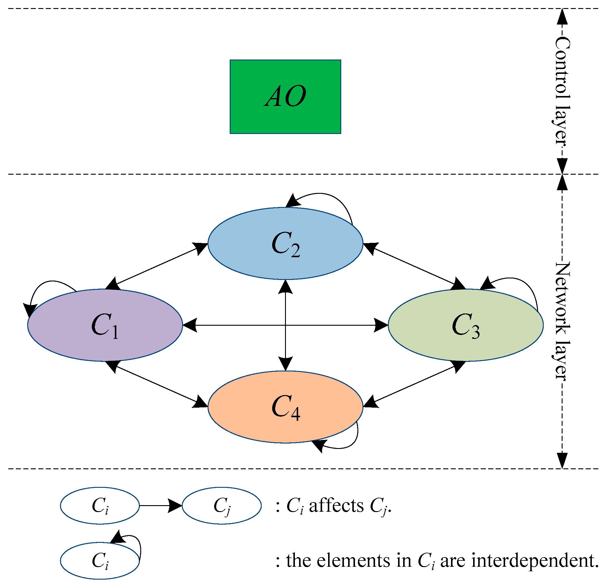
In ANP [11], the system elements are divided into two parts: (1) The first is called the control layer, including the problem objective and decision criteria. All decision criteria are considered independent of each other and are governed only by the problem objective. There can be no decision criteria in the control layer, but at least one objective; (2) The second part is the network layer, which is composed of all the elements that are controlled by the control layer, and its internal network structure is interacted.

Therefore, we set up the ANP structure of green supplier assessment as shown in Figure 2. The control layer only has one element: the green supplier assessment objective (AO), and the network layer has four element groups: product attribute (C₁), internal competitiveness (C₂), external competitiveness (C₃) and cooperation ability (C₄). Each element group affects each other and contains different elements. The elements in the same element group also affect each other. For example, internal competitiveness (C₂) is affected by product attribute (C₁), external competitiveness (C₃) and cooperation ability (C₄), and innovation capacity (C_2,1), manufacturing capacity (C_2,2) and agility capacity (C_2,3) also affect each other.

According to the ANP structure of green supplier assessment shown in Figure 2, the control layer has the element AO and the network layer has the element groups C₁, C₂, …, C_N (here, N = 4). The element group C_i (i = 1, 2, …, N) contains the elements $C_{i,1},C_{i,2},\dots ,C_{i,n_i}$. The control layer element AO is taken as the criterion and the element $C_{j,l}$ (l = 1, 2, …, $n_j$) in $C_j$ (j = 1, 2, …, N) is taken as the sub-criterion. Based on the influence of the elements in C_i on $C_{j,l}$, the indirect dominance comparison of the elements in C_i are conducted.

Here, the influence of the elements in C_i on $C_{j,l}$ are assessed according to the personal experience and subjective judgment of experts, so using exact numbers to describe the influence of the elements in C_i on $C_{j,l}$ is unreasonable. In contrast, the fuzzy number can reflect the inherent uncertainty of the expert’s preference. At the same time, when integrating the opinions of multiple experts, the assessment of the influence of the elements in C_i on $C_{j,l}$ by experts is obviously with indiscernibility. The rough boundary interval in rough sets theory [26,27,28,29] can describe the indiscernibility as a set boundary area instead of a membership function, which can better integrate the assessment of multiple experts.

Based the index weight obtaining method in Reference [30], we design a rough ANP method to determine the index weight in green supplier assessment. The specific process of the designed rough ANP is as follows.

Step 1: Under the control layer element AO, we conduct the indirect dominance comparison of the elements in C_i according to their influence on $C_{j,l}$.

There are q experts participating in the indirect dominance comparison of the elements in C_i. The fuzzy reciprocal judgement matrix $E^{k,i,(j,l)}={(e_{g,h}^{k,i,(j,l)})}_{n_i\times n_i}$ given by the expert k (k = 1, 2, …, q) is as follows:

$$E^{k,i,(j,l)}=\begin{array}{ccccc}{C}_{j,l}& C_{i,1}& C_{i,2}& \cdots & C_{i,n_i}\\ C_{i,1}& 1& e_{1,2}^{k,i,(j,l)}& \cdots & e_{1,n_i}^{k,i,(j,l)}\\ C_{i,2}& e_{2,1}^{k,i,(j,l)}& 1& \cdots & e_{2,n_i}^{k,i,(j,l)}\\ ⋮& ⋮& ⋮& & ⋮\\ C_{i,n_i}& e_{n_i,1}^{k,i,(j,l)}& e_{n_i,2}^{k,i,(j,l)}& \cdots & 1\end{array}$$

(1)

where $e_{g,h}^{k,i,(j,l)}$ represents the indirect dominance score of the element $C_{i,h}$ compared to the element $C_{i,g}$ giver by the expert k, here g,h = 1, 2, …, n_i and g ≠ h. $e_{g,h}^{k,i,(j,l)}$ is a trapezoidal fuzzy number and $e_{g,h}^{k,i,(j,l)}=(a_{g,h}^{k,i,(j,l)},b_{g,h}^{k,i,(j,l)},c_{g,h}^{k,i,(j,l)},d_{g,h}^{k,i,(j,l)})$. $a_{g,h}^{k,i,(j,l)},b_{g,h}^{k,i,(j,l)},c_{g,h}^{k,i,(j,l)}$ and $d_{g,h}^{k,i,(j,l)}$ are all positive real numbers and $a_{g,h}^{k,i,(j,l)}\le b_{g,h}^{k,i,(j,l)}\le c_{g,h}^{k,i,(j,l)}\le d_{g,h}^{k,i,(j,l)}$. Then the consistency of the matrix given by each expert is verified. If it is qualified, the next step will be carried out; otherwise, this step will be returned.

Then, $E^{k,i,(j,l)}$ is split into $A^{k,i,(j,l)}={(a_{g,h}^{k,i,(j,l)})}_{n_i\times n_i}$, $B^{k,i,(j,l)}={(b_{g,h}^{k,i,(j,l)})}_{n_i\times n_i}$, $C^{k,i,(j,l)}={(c_{g,h}^{k,i,(j,l)})}_{n_i\times n_i}$ and $D^{k,i,(j,l)}={(d_{g,h}^{k,i,(j,l)})}_{n_i\times n_i}$. Based on $A^{1,i,(j,l)},A^{2,i,(j,l)},\dots ,A^{q,i,(j,l)}$, the rough group decision matrix $A^{i,(j,l)}={(a_{g,h}^{i,(j,l)})}_{n_i\times n_i}$ is constructed where $a_{g,h}^{i,(j,l)}=\{a_{g,h}^{1,i,(j,l)},a_{g,h}^{2,i,(j,l)},\dots ,a_{g,h}^{q,i,(j,l)}\}$, g,h = 1, 2, …, n_i and g ≠ h.

The rough boundary interval of $a_{g,h}^{k,i,(j,l)}\in a_{g,h}^{i,(j,l)}$ (k = 1, 2, …, q) is $RN(a_{g,h}^{k,i,(j,l)})=\left[a_{g,h}^{k,i,(j,l),-},a_{g,h}^{k,i,(j,l),+}\right]$ where $a_{g,h}^{k,i,(j,l),-},a_{g,h}^{k,i,(j,l),+}$ are the rough lower limit and rough upper limit of $a_{g,h}^{k,i,(j,l)}$ in the set $a_{g,h}^{i,(j,l)}$.

Thus, the rough boundary interval of $a_{g,h}^{i,(j,l)}$ can be expressed as $RN(a_{g,h}^{i,(j,l)})=\left\{\left[a_{g,h}^{1,i,(j,l),-},a_{g,h}^{1,i,(j,l),+}\right],\left[a_{g,h}^{2,i,(j,l),-},a_{g,h}^{2,i,(j,l),+}\right],\cdots ,\left[a_{g,h}^{q,i,(j,l),-},a_{g,h}^{q,i,(j,l),+}\right]\right\}$. According to the calculation rule of rough boundary interval, the mean form of $RN(a_{g,h}^{i,(j,l)})$ can be obtained as $Avg\_RN(a_{g,h}^{i,(j,l)})=\left[a_{g,h}^{i,(j,l),-},a_{g,h}^{i,(j,l),+}\right]=\left[{\displaystyle \sum _{k=1}^q{a}_{g,h}^{k,i,(j,l),-}}/q,{\displaystyle \sum _{k=1}^q{a}_{g,h}^{k,i,(j,l),+}}/q\right]$ where $a_{g,h}^{i,(j,l),-},a_{g,h}^{i,(j,l),+}$ are the rough lower limit and rough upper limit of the set $a_{g,h}^{i,(j,l)}$.

The rough judgement matrix is constructed as $E{A}^{i,(j,l)}={(Avg\_RN(a_{g,h}^{i,(j,l)}))}_{n_i\times n_i}$. Then, $E{A}^{i,(j,l)}$ is split into the rough lower limit matrix $E{A}^{i,(j,l),-}={(a_{g,h}^{i,(j,l),-})}_{n_i\times n_i}$ and the rough upper limit matrix $E{A}^{i,(j,l),+}={(a_{g,h}^{i,(j,l),+})}_{n_i\times n_i}$.

The eigenvectors corresponding to the maximum eigenvalues of $E{A}^{i,(j,l),-}$ and $E{A}^{i,(j,l),+}$ are $V{A}_{}^{i,(j,l),-}={\left[v{a}_1^{i,(j,l),-},v{a}_2^{i,(j,l),-},\cdots ,v{a}_{n_i}^{i,(j,l),-}\right]}^{\mathrm{T}}$ and $V{A}_{}^{i,(j,l),+}={\left[v{a}_1^{i,(j,l),+},v{a}_2^{i,(j,l),+},\cdots ,v{a}_{n_i}^{i,(j,l),+}\right]}^{\mathrm{T}}$ respectively, where $v{a}_h^{i,(j,l),-},v{a}_h^{i,(j,l),+}$ are the value of $V{A}_{}^{i,(j,l),-}$ and $V{A}_{}^{i,(j,l),+}$ on the h (h = 1, 2, …, n_i) dimension. Then, a set $G{A}^{i,(j,l)}=\{g{a}_1^{i,(j,l)},g{a}_2^{i,(j,l)},\dots ,g{a}_{n_i}^{i,(j,l)}\}$ can be obtained where $g{a}_h^{i,(j,l)}=(|v{a}_h^{i,(j,l),-}|+|v{a}_h^{i,(j,l),+}|)/2$. Similarly, we also get the other sets: $G{B}^{i,(j,l)}=\{g{b}_1^{i,(j,l)},g{b}_2^{i,(j,l)},\dots ,g{b}_{n_i}^{i,(j,l)}\}$, $G{C}^{i,(j,l)}=\{g{c}_1^{i,(j,l)},g{c}_2^{i,(j,l)},\dots ,g{c}_{n_i}^{i,(j,l)}\}$ and $G{D}^{i,(j,l)}=\{g{d}_1^{i,(j,l)},g{d}_2^{i,(j,l)},\dots ,g{d}_{n_i}^{i,(j,l)}\}$.

Thereupon, the eigenvector $w_{}^{i,(j,l)}={[w_1^{i,(j,l)},w_2^{i,(j,l)},\dots ,w_{n_i}^{i,(j,l)}]}^{\mathrm{T}}$ is obtained, where $w_h^{i,(j,l)}=\frac{[{(g{d}_h^{i,(j,l)})}^2+g{d}_h^{i,(j,l)}\cdot g{c}_h^{i,(j,l)}+{(g{c}_h^{i,(j,l)})}^2]-[{(g{a}_h^{i,(j,l)})}^2+g{a}_h^{i,(j,l)}\cdot g{b}_h^{i,(j,l)}+{(g{b}_h^{i,(j,l)})}^2]}{3(g{d}_h^{i,(j,l)}+g{c}_h^{i,(j,l)}-g{a}_h^{i,(j,l)}-g{b}_h^{i,(j,l)})}$, h = 1, 2, …, n_i. Then, the eigenvector $w_{}^{i,(j,l)}={[w_1^{i,(j,l)},w_2^{i,(j,l)},\dots ,w_{n_i}^{i,(j,l)}]}^{\mathrm{T}}$ is normalized as ${\omega }_{}^{i,(j,l)}={[{\omega }_1^{i,(j,l)},{\omega }_2^{i,(j,l)},\dots ,{\omega }_{n_i}^{i,(j,l)}]}^{\mathrm{T}}$ where ${\omega }_h^{i,(j,l)}=w_h^{i,(j,l)}/{\displaystyle \sum _{h=1}^{n_i}{w}_h^{i,(j,l)}}$.

Step 2: We represent ${\Omega }^{i,j}={({\omega }_h^{i,(j,l)})}_{n_i\times n_j}$ as follows:

$${\Omega }^{i,j}=\left[\begin{array}{cccc}{\omega }_1^{i,(j,1)}& {\omega }_1^{i,(j,2)}& \cdots & {\omega }_1^{i,(j,n_j)}\\ {\omega }_2^{i,(j,1)}& {\omega }_2^{i,(j,2)}& \cdots & {\omega }_2^{i,(j,n_j)}\\ ⋮& ⋮& & ⋮\\ {\omega }_{n_i}^{i,(j,1)}& {\omega }_{n_i}^{i,(j,2)}& \cdots & {\omega }_{n_i}^{i,(j,n_j)}\end{array}\right]$$

(2)

where the column vector ${\omega }_{}^{i,(j,l)}$ is the normalized influence degree sorting vector of the elements $C_{i,1},C_{i,2},\dots ,C_{i,n_i}$ in $C_i$ on the element $C_{j,l}$ in $C_j$. If the elements in $C_j$ is not affected by the elements in $C_i$, ${\Omega }^{i,j}=0$.

So we get the hyper-matrix $\Omega$ under the control layer element AO as follows:

$$\begin{array}{l}\begin{array}{cccccccccccccccccccccc}& & & & & & & & & & C_1& & & & C_2& & & & & & C_N& \\ & & & & & & & & & C_{1,1}& \cdots & C_{1,n_1}& & C_{2,1}& \cdots & C_{2,n_2}& & \cdots & & C_{N,1}& \cdots & C_{N,n_N}\end{array}\\ \Omega =\begin{array}{cc}& C_{1,1}\\ C_1& ⋮\\ & C_{1,n_1}\\ & \\ & C_{2,1}\\ C_2& ⋮\\ & C_{2,n_2}\\ & \\ ⋮& ⋮\\ & \\ & C_{N,1}\\ C_N& ⋮\\ & C_{N,n_N}\end{array}\left[\begin{array}{cccc}& & & \\ {\Omega }^{1,1}& {\Omega }^{1,2}& \cdots & {\Omega }^{1,N}\\ & & & \\ & & & \\ & & & \\ {\Omega }^{2,1}& {\Omega }^{2,2}& \cdots & {\Omega }^{2,N}\\ & & & \\ & & & \\ ⋮& ⋮& & ⋮\\ & & & \\ & & & \\ {\Omega }^{N,1}& {\Omega }^{N,2}& \cdots & {\Omega }^{N,N}\\ & & & \end{array}\right]\end{array}$$

(3)

Step 3: The sub-block ${\Omega }^{i,j}$ of $\Omega$ is column normalized, but $\Omega$ isn’t column normalized. To solve this problem, we conduct the indirect dominance comparison of the element groups $C_1,C_2,\dots ,C_N$ according to their influence on $C_j$ $(j=1,2,\dots ,N)$ under the control layer element AO. Here, we adopt a similar approach to Step 1 and get the relative importance matrix $\Psi ={({\psi }^{i,j})}_{N\times N}$ of element groups as follows:

$$\Psi =\left[\begin{array}{cccc}{\psi }^{1,1}& {\psi }^{1,2}& \cdots & {\psi }^{1,N}\\ {\psi }^{2,1}& {\psi }^{2,2}& \cdots & {\psi }^{2,N}\\ ⋮& ⋮& & ⋮\\ {\psi }^{N,1}& {\psi }^{N,2}& \cdots & {\psi }^{N,N}\end{array}\right]$$

(4)

where the column vector ${\psi }^{,j}={[{\psi }^{1,j},{\psi }^{2,j},\dots ,{\psi }^{N,j}]}^{\mathrm{T}}$ is the normalized influence degree sorting vector of the element groups $C_1,C_2,\dots ,C_N$ on $C_j$.

The weighted form of the hyper-matrix $\Omega$ is $\overline{\Omega }$, where ${\overline{\Omega }}^{i,j}={\psi }^{i,j}{\Omega }^{i,j}$ $(i=1,2,\dots ,N,j=1,2,\dots ,N)$.

Step 4: We do the square operation of the weighted hyper-matrix $\overline{\Omega }$ until the result converges to a stable limit hyper-matrix ${\overline{\Omega }}^{\infty }$ as follows:

$${\overline{\Omega }}^{\infty }=\underset{t\to \infty }{\lim }{\overline{\Omega }}^t$$

(5)

Any column of ${\overline{\Omega }}^{\infty }$ is the limit relative ranking vector of all elements in the network layer. So we can get the weight vector of the index system shown in Figure 1 as follows:

$$\theta ={[{\theta }_{1,1},{\theta }_{1,2},\dots ,{\theta }_{1,n_1},{\theta }_{2,1},{\theta }_{2,2},\dots ,{\theta }_{2,n_2},{\theta }_{3,1},{\theta }_{3,2},\dots ,{\theta }_{3,n_3},{\theta }_{4,1},{\theta }_{4,2},\dots ,{\theta }_{4,n_4}]}^{\mathrm{T}}$$

(6)

where ${\theta }_{j,1},{\theta }_{j,2},\dots ,{\theta }_{j,n_j}$ are the weights of $C_{j,1},C_{j,2},\dots ,C_{j,n_j}$, $j=1,2,\dots ,N$.

Furtherly, the weight of $C_j$ ($j=1,2,\dots ,N$) is obtained as follows:

$${\theta }_j={\displaystyle \sum _{l=1}^{n_j}{\theta }_{j,l}}$$

(7)

5. Green Supplier Assessment

5.1. Related Concepts of Evidence Theory

We assume that there are M suppliers to be assessed. Based on evidence theory [31,32], the set of the suppliers to be assessed is defined as the identification framework $\Theta =\{x_1,x_2,\dots ,x_M\}$. All possible sets in $\Theta$ are represented by the power set $2^{\Theta }$. If each element in $\Theta$ is incompatible with each other, the number of elements in $2^{\Theta }$ is $2^M$. Then, a set function $mass:2^{\Theta }\to [0,1]$, which satisfies $mass(\varphi )=0$ and ${\displaystyle \sum _{\phi \subset \Theta }mass(\phi )}=1$, is defined. The set function $mass$ is known as the basic probability distribution function on $\Theta$. Here, $\phi$ represents a supplier to be assessed. $mass(\phi )$ is the basic probability distribution value of $\phi$ and represents the trust degree for $\Phi$, Any supplier to be assessed satisfying the condition “$mass(\phi )>0$” is called a focal element.

For $\phi ,{\phi }_1,{\phi }_2,\dots ,{\phi }_n\subseteq \Theta$, the fusion rule of the basic probability distribution functions $mas{s}_1,mas{s}_2,\dots ,mas{s}_n$ on $\Theta$ is as follows:

$$mass(\phi )=\frac{1}{K}{\displaystyle \sum _{{\phi }_1\cap {\phi }_2\cap \dots \cap {\phi }_n=\varnothing }mas{s}_1({\phi }_1)\cdot mas{s}_2({\phi }_2)\cdot \dots \cdot mas{s}_n({\phi }_n)}$$

(8)

where $mass=mas{s}_1\oplus mas{s}_2\oplus \dots \oplus mas{s}_n$.

The normalization constant K is defined as follows:

$$K={\displaystyle \sum _{{\phi }_1\cap {\phi }_2\cap \dots \cap {\phi }_n\ne \varnothing }mas{s}_1({\phi }_1)\cdot mas{s}_2({\phi }_2)\cdot \dots \cdot mas{s}_n({\phi }_n)}$$

(9)

The total trust degree of $\phi$ on $\Theta$ can be expressed as the belief function $Bel(\phi )={\displaystyle \sum _{\varphi \subset \Theta ,\varphi \subseteq \phi }mass(\varphi )}$, and the uncertainty degree of $\phi$ on $\Theta$ can be expressed as the plausible function $Pl(\phi )={\displaystyle \sum _{\varphi \subset \Theta ,\varphi \cap \phi \ne \varnothing }mass(\varphi )}$. For a supplier $\phi$ on $\Theta$, $Bel(\phi )$ represents the sum of the possibility measurement for all subsets of $\phi$, and $Pl(\phi )$ represents the sum of the uncertainty measurement for all subsets of $\phi$. The confirmation degree of $\phi$ is represented by the trust interval $[Bel(\phi ),Pl(\phi )]$.

Therefore, $Bel(\phi )$ reflects the sum of exact reliability which the evidences support $\phi$, and $Pl(\phi )$ reflects the sum of reliability which the evidences do not negate $\phi$. As a result, $Bel(\phi )$ and $Pl(\phi )$ can be considered as the minimum and maximum probability bounds respectively, so $[Bel(\phi ),Pl(\phi )]$ can form the trust interval.

Based on the above analysis, assessing the suppliers by trust interval is more reliable than by maximum belief function or maximum plausible function [30,31]. We assume that the supplier ${\phi }_s$ is better than supplier ${\phi }_y$ with a degree of ${\epsilon }_{s,y}$ ($0\le {\epsilon }_{s,y}\le 1$). If the trust intervals of ${\phi }_s$ and ${\phi }_y$ are $[Bel({\phi }_s),Pl({\phi }_s)]$ and $[Bel({\phi }_y),Pl({\phi }_y)]$ respectively, ${\epsilon }_{s,y}$ is defined as follows:

$${\epsilon }_{s,y}=\frac{\max \{0,Pl({\phi }_s)-Bel({\phi }_y)\}-\max \{0,Bel({\phi }_s)-Pl({\phi }_y)\}}{(Pl({\phi }_s)-Bel({\phi }_s))+(Pl({\phi }_y)-Bel({\phi }_y))}$$

(10)

The decision rules based on trust interval are as follows:

• If ${\epsilon }_{s,y}>0.5$, ${\phi }_s$ is better than ${\phi }_y$ (recorded as ${\phi }_s⊳{\phi }_y$);
• If ${\epsilon }_{s,y}<0.5$, ${\phi }_s$ is worse than ${\phi }_y$ (recorded as ${\phi }_s⊲{\phi }_y$);
• If ${\epsilon }_{s,y}=0.5$, ${\phi }_s$ and ${\phi }_y$ are equal (recorded as ${\phi }_s={\phi }_y$);
• For three suppliers ${\phi }_s$, ${\phi }_y$ and ${\phi }_z$, if ${\epsilon }_{s,y}>0.5$ and ${\epsilon }_{y,z}>0.5$, ${\phi }_s$ is better than ${\phi }_y$ and ${\phi }_y$ is better than ${\phi }_z$, so ${\phi }_s⊳{\phi }_y⊳{\phi }_z$.

5.2. Green Supplier Assessing Procedure

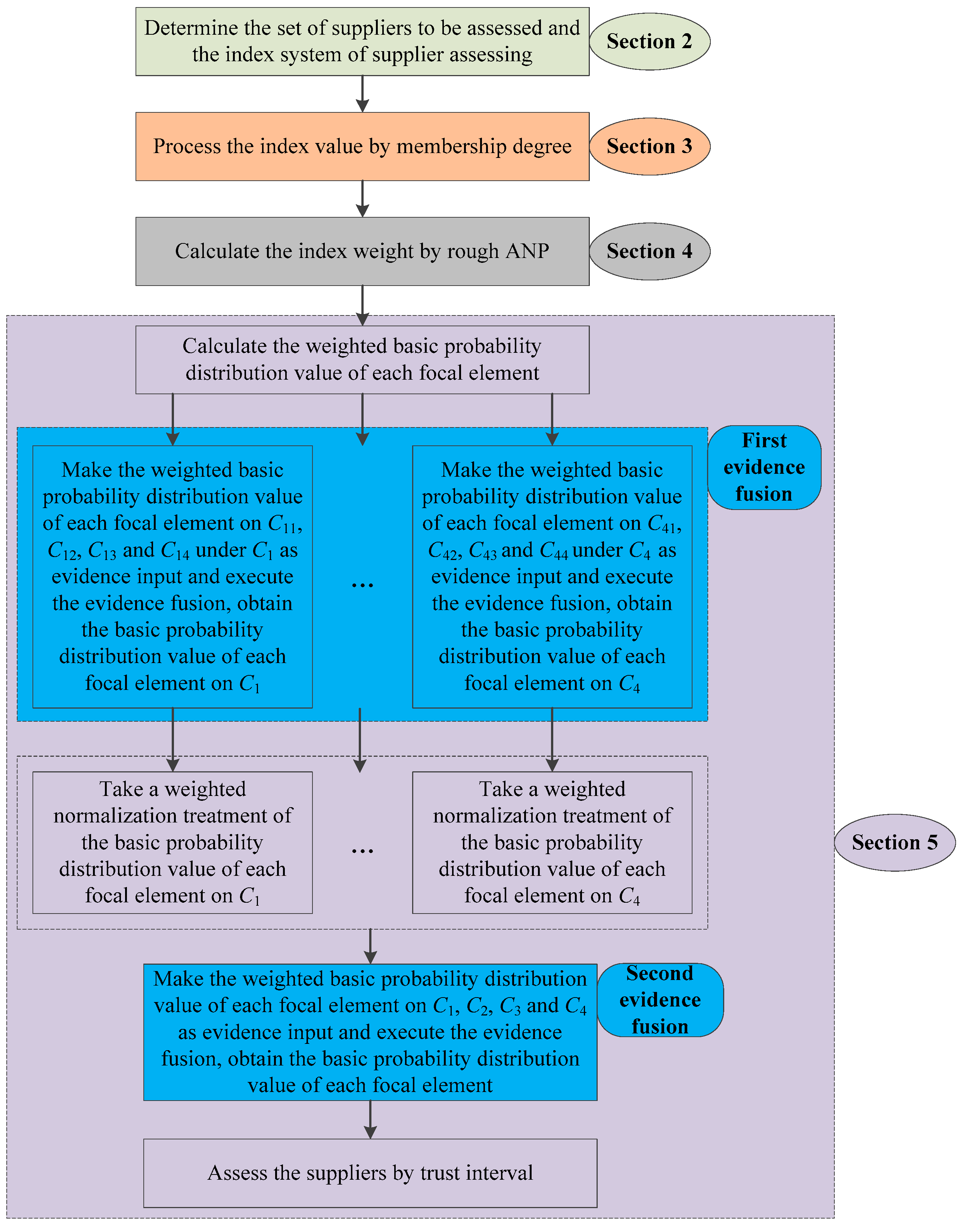
On the index $C_{j,l}$, the weighted basic probability distribution value of the focal element ${\phi }_s$ (s < 2^N) is represented as ${mass}_{C_{j,l}}^{\prime }({\phi }_s)$. In this paper, we use ${mass}_{C_{j,l}}^{\prime }({\phi }_s)$ as the evidence input of green supplier assessment.

The utility value of each focal element except $\Theta$ can be calculated through index value processing. The special focal element $\Theta$ can indicate the uncertainty of the expert on an index. If we don’t consider the influence of $\Theta$, the green supplier assessment problem will become a simple probability distribution problem, and the advantages of evidence theory will not be applied. Meanwhile, the trust degree of expert in each index is different and the uncertainty of index is reflected by the probability distribution of $\Theta$. Thus the probability distribution value of $\Theta$ on different indexes should also be treated differently.

In the green supplier assessment problem, the index weight is obviously not fixed in the case of different requirements. When costs need to be reduced, C₁₁ is more important than other indexes and its weight must be higher than other indexes, and the basic probability distribution value of $\Theta$ on C₁₁ should be smaller than other indexes. Therefore, the index weight calculated by rough ANP is introduced to adjust the preference of experts and solve the probability distribution problem of $\Theta$ on different indexes. Then, the weighted basic probability distribution value of each focal element on each index is obtained as ${mass}_{C_{j,l}}^{\prime }({\phi }_s)$.

We take a weighted normalization treatment for the basic probability distribution values of all focal elements and calculate ${mass}_{C_{j,l}}^{\prime }({\phi }_s)$, as follows:

$$\{\begin{array}{ll}{mass}_{C_{j,l}}^{\prime }({\phi }_s)={\theta }_{j,l}\frac{{\tau }_{s,(j,l)}}{{\displaystyle \sum _{s=1}^{l-1}{\tau }_{s,(j,l)}}},& {\phi }_s\ne \Theta \\ {mass}_{C_{j,l}}^{\prime }({\phi }_s)=1-{\theta }_{j,l},& {\phi }_s=\Theta \end{array}$$

(11)

Based on the two-level index system shown in Figure 1, we establish a two-order fusion evidence theory model for green supplier assessment. The procedure is shown in Figure 3.

6. Case Study

6.1. An Application Case of Bearing Cage Supplier Assessment

For a bearing manufacturing enterprise, there are three bearing cage suppliers to be assessed. The set of suppliers to be assessed is $\{{\phi }_1,{\phi }_2,{\phi }_3\}$. The best bearing cage supplier need to be selected after green supplier assessment. The index value of quantitative type (C₁₁ and C₁₂) is obtained directly from the enterprise resources planning system (ERP) of the bearing manufacturing enterprise, and the index value of qualitative type (other indexes) is obtained by the method of expert’s scoring (i.e., 0.1, 0.3, 0.5, 0.7 and 0.9). The index values of three bearing cage suppliers are shown in

Table 1. The index values of three bearing cage suppliers.

Supplier	C1,1	C1,2	C1,3	C1,4	C2,1	C2,2	C2,3	C3,1	C3,2	C3,3	C3,4	C4,1	C4,2	C4,3	C4,4
${\phi }_1$	6.4 × 101	0.01	0.7	0.1	[0.1, 0.3]	0.5	0.7	0.5	0.5	0.7	0.7	/	[0.7, 0.9]	0.5	0.7
${\phi }_2$	1.9 × 103	0.01	0.9	0.7	0.5	0.7	0.9	/	0.7	[0.5, 0.7]	0.9	0.7	0.5	0.7	0.9
${\phi }_3$	2.8 × 104	0.03	0.1	0.7	0.7	0.1	0.3	0.1	0.5	0.1	0.3	0.1	0.5	/	0.1

. The units of the index value on $C_{1,1}$ and $C_{1,2}$ are RMB and mm (error value) respectively.

Then, the normalized index values of three bearing cage suppliers are shown in

Table 2. The normalized index values of three bearing cage suppliers.

Supplier	C1,1	C1,2	C1,3	C1,4	C2,1	C2,2	C2,3	C3,1	C3,2	C3,3	C3,4	C4,1	C4,2	C4,3	C4,4
${\phi }_1$	0.0023	1.0000	0.7778	0.1429	[0.1429, 0.4286]	0.7143	0.7778	1.0000	0.7143	1.0000	0.7778	/	[0.7778, 1.0000]	0.7143	0.7778
${\phi }_2$	0.0669	1.0000	1.0000	1.0000	0.7143	1.0000	1.0000	/	1.0000	[0.7143, 1.0000]	1.0000	1.0000	0.5556	1.0000	1.0000
${\phi }_3$	1.0000	0.3333	0.1111	1.0000	1.0000	0.1429	0.3333	0.2000	0.7143	0.1429	0.3333	0.1429	0.5556	/	0.1111

.

Five comment levels: very bad (G₁), bad (G₂), middle (G₃), good (G₄) and very good (G₅) are set. Taking the normalized index values $v_{1,(1,1)}^{\prime }=0.0023$, $v_{2,(1,1)}^{\prime }=0.0669$ and $v_{3,(1,1)}^{\prime }=1.0000$ for an example, we can get $v_{(1,1)}^{\prime }(G_1)=0.0023$ and $v_{(1,1)}^{\prime }(G_5)=1.0000$, so $v_{(1,1)}^{\prime }(G_2)=0.2517$, $v_{(1,1)}^{\prime }(G_3)=0.5011$ and $v_{(1,1)}^{\prime }(G_4)=0.7506$. The corresponding numbers of the five comment levels are ${\pi }_1=0.1,{\pi }_2=0.3,{\pi }_3=0.5,{\pi }_4=0.7$ and ${\pi }_5=0.9$. To the normalized index value $v_{2,(1,1)}^{\prime }=0.0669$, the membership degrees are ${\beta }_1=0.7410$ and ${\beta }_2=0.2590$, so ${\tau }_{2,(1,1)}={\beta }_1{\pi }_1+{\beta }_2{\pi }_2=0.0648$. The utility values of three bearing cage suppliers are shown in

Table 3. The utility values of three bearing cage suppliers.

Supplier	C1,1	C1,2	C1,3	C1,4	C2,1	C2,2	C2,3	C3,1	C3,2	C3,3	C3,4	C4,1	C4,2	C4,3	C4,4
${\phi }_1$	0.1000	0.9000	0.7778	0.1000	0.2857	0.6333	0.6334	0.9000	0.1000	0.9000	0.6334	/	0.8889	0.1000	0.7000
${\phi }_2$	0.1518	0.9000	0.9000	0.9000	0.6333	0.9000	0.9000	/	0.9000	0.8572	0.9000	0.9000	0.1000	0.9000	0.9000
${\phi }_3$	0.9000	0.1000	0.1000	0.9000	0.9000	0.1000	0.1000	0.1000	0.1000	0.1000	0.1000	0.1000	0.1000	/	0.1000

.

Next, the index weight is calculated by rough ANP. There are four experts: expert 1, expert 2, expert 3 and expert 4.

Taking the indirect dominance comparison of the elements in $C_1$ according to their influence on $C_{2,1}$ under the control layer element AO for an example, the fuzzy reciprocal judgement matrices given by the four experts are shown as follows:

$$E^{1,1,(2,1)}=\begin{array}{ccccc}{C}_{2,1}& C_{1,1}& C_{1,2}& C_{1,3}& C_{1,4}\\ C_{1,1}& (1,1,1,1)& (1,11/9,13/7,7/3)& (1,11/9,13/7,7/3)& (3/2,13/7,3,4)\\ C_{1,2}& (3/7,7/13,9/11,1)& (1,1,1,1)& (1,11/9,13/7,7/3)& (1,11/9,13/7,7/3)\\ C_{1,3}& (3/7,7/13,9/11,1)& (3/7,7/13,9/11,1)& (1,1,1,1)& (1,11/9,13/7,7/3)\\ C_{1,4}& (1/4,1/3,7/13,2/3)& (3/7,7/13,9/11,1)& (3/7,7/13,9/11,1)& (1,1,1,1)\end{array},$$

$$E^{2,1,(2,1)}=\begin{array}{ccccc}{C}_{2,1}& C_{1,1}& C_{1,2}& C_{1,3}& C_{1,4}\\ C_{1,1}& (1,1,1,1)& (1,1,1,1)& (1,11/9,13/7,7/3)& (1,11/9,13/7,7/3)\\ C_{1,2}& (1,1,1,1)& (1,1,1,1)& (1,11/9,13/7,7/3)& (1,11/9,13/7,7/3)\\ C_{1,3}& (3/7,7/13,9/11,1)& (3/7,7/13,9/11,1)& (1,1,1,1)& (1,1,1,1)\\ C_{1,4}& (3/7,7/13,9/11,1)& (3/7,7/13,9/11,1)& (1,1,1,1)& (1,1,1,1)\end{array},$$

$$E^{3,1,(2,1)}=\begin{array}{ccccc}{C}_{2,1}& C_{1,1}& C_{1,2}& C_{1,3}& C_{1,4}\\ C_{1,1}& (1,1,1,1)& (3/2,13/7,3,4)& (1,1,1,1)& (1,11/9,13/7,7/3)\\ C_{1,2}& (1/4,1/3,7/13,2/3)& (1,1,1,1)& (1/4,1/3,7/13,2/3)& (3/7,7/13,9/11,1)\\ C_{1,3}& (1,1,1,1)& (3/2,13/7,3,4)& (1,1,1,1)& (1,11/9,13/7,7/3)\\ C_{1,4}& (3/7,7/13,9/11,1)& (1,11/9,13/7,7/3)& (3/7,7/13,9/11,1)& (1,1,1,1)\end{array},$$

$$E^{4,1,(2,1)}=\begin{array}{ccccc}{C}_{2,1}& C_{1,1}& C_{1,2}& C_{1,3}& C_{1,4}\\ C_{1,1}& (1,1,1,1)& (1,11/9,13/7,7/3)& (3/2,13/7,3,4)& (7/3,3,17/3,9)\\ C_{1,2}& (3/7,7/13,9/11,1)& (1,1,1,1)& (1,11/9,13/7,7/3)& (3/2,13/7,3,4)\\ C_{1,3}& (1/4,1/3,7/13,2/3)& (3/7,7/13,9/11,1)& (1,1,1,1)& (1,11/9,13/7,7/3)\\ C_{1,4}& (1/9,3/17,1/3,3/7)& (1/4,1/3,7/13,2/3)& (3/7,7/13,9/11,1)& (1,1,1,1)\end{array}.$$

We check the consistency of $E^{1,1,(2,1)},E^{2,1,(2,1)},E^{3,1,(2,1)}$ and $E^{4,1,(2,1)}$ and all of them are qualified.

Then, $E^{k,1,(2,1)}$($k=1,2,3,4$) is split into $A^{k,1,(2,1)}={(a_{g,h}^{k,1,(2,1)})}_{4\times 4}$, $B^{k,1,(2,1)}={(b_{g,h}^{k,1,(2,1)})}_{4\times 4}$, $C^{k,1,(2,1)}={(c_{g,h}^{k,1,(2,1)})}_{4\times 4}$ and $D^{k,1,(2,1)}={(d_{g,h}^{k,1,(2,1)})}_{4\times 4}$. For example, $A^{1,1,(2,1)}={(a_{g,h}^{1,1,(2,1)})}_{4\times 4}$ is as follows:

$$A^{1,1,(2,1)}=\left[\begin{array}{cccc}1& 1& 1& 3/2\\ 3/7& 1& 1& 1\\ 3/7& 3/7& 1& 1\\ 1/4& 3/7& 3/7& 1\end{array}\right].$$

Based on $A^{1,1,(2,1)},A^{2,1,(2,1)},A^{3,1,(2,1)},A^{4,1,(2,1)}$, the rough group decision matrix $A^{1,(2,1)}={(a_{g,h}^{1,(2,1)})}_{4\times 4}$ is constructed as follows:

$$A^{1,(2,1)}=\left[\begin{array}{cccc}\{1,1,1,1\}& \{1,1,3/2,1\}& \{1,1,1,3/2\}& \{3/2,1,1,7/3\}\\ \{3/7,1,1/4,3/7\}& \{1,1,1,1\}& \{1,1,1/4,1\}& \{1,1,3/7,3/2\}\\ \{3/7,3/7,1,1/4\}& \{3/7,3/7,3/2,3/7\}& \{1,1,1,1\}& \{1,1,1,1\}\\ \{1/4,3/7,3/7,1/9\}& \{3/7,3/7,1,1/4\}& \{3/7,1,3/7,3/7\}& \{1,1,1,1\}\end{array}\right].$$

For the partition $a_{1,4}^{1,1,(2,1)}$ = 3/2 in the element $a_{1,4}^{1,(2,1)}=\left\{3/2,1,1,7/3\right\}$, its upper approximation set is {3/2, 7/3} and lower approximation set is {3/2, 1, 1}, then $\underset{\_}{L}(a_{1,4}^{1,1,(2,1)})$ = (3/2 + 1 + 1)/3 = 1.17, $\overline{L}(a_{1,4}^{1,1,(2,1)})$ = (3/2 + 7/3)/2 = 1.92 and $RN(a_{1,4}^{1,1,(2,1)})$ = [1.17, 1.92]. Similarly, $RN(a_{1,4}^{2,1,(2,1)})=RN(a_{1,4}^{3,1,(2,1)})$ = [1, 1.46], $RN(a_{1,4}^{4,1,(2,1)})$ = [1.46, 2.33]. So $RN(a_{1,4}^{1,(2,1)})$ = {[1.17, 1.92], [1, 1.46], [1, 1.46], [1.46, 2.33]}.

According to the calculation rule of rough boundary interval, the mean form of $RN(a_{1,4}^{1,(2,1)})$ is obtained as $Avg\_RN(a_{1,4}^{1,(2,1)})$ = [1.16, 1.79]. Then, the rough judgement matrix $E{A}^{1,(2,1)}={(Avg\_RN(a_{g,h}^{1,(2,1)}))}_{4\times 4}$ is constructed as follows:

$$E{A}^{1,(2,1)}=\left[\begin{array}{cccc}[1,1]& [1.03,1.22]& [1.03,1.22]& [1.16,1.79]\\ [0.38,0.74]& [1,1]& [0.67,0.95]& [0.72,1.17]\\ [0.38,0.74]& [0.50,0.90]& [1,1]& [1,1]\\ [0.23,0.38]& [0.38,0.74]& [0.46,0.68]& [1,1]\end{array}\right].$$

$E{A}^{1,(2,1)}$ is split into the rough lower limit matrix $E{A}^{1,(2,1),-}={(a_{g,h}^{1,(2,1),-})}_{4\times 4}$ and the rough upper limit matrix $E{A}^{1,(2,1),+}={(a_{g,h}^{1,(2,1),+})}_{4\times 4}$. The eigenvectors corresponding to the maximum eigenvalues of $E{A}^{1,(2,1),-}$ and $E{A}^{1,(2,1),+}$ are $V{A}_{}^{1,(2,1),-}$ = [0.71, 0.44, 0.45, 0.30]^T and $V{A}_{}^{1,(2,1),+}$ = [0.65, 0.49, 0.47, 0.34]^T respectively. Then, we get a set $G{A}^{1,(2,1)}$ = {0.68, 0.47, 0.46, 0.32}. Similarly, we also get the other sets: $G{B}^{1,(2,1)}$ = {0.73, 0.51, 0.66, 0.58}, $G{C}^{1,(2,1)}$ = {0.82, 0.67, 0.73, 0.69} and $G{D}^{1,(2,1)}$ = {0.95, 0.77, 0.83, 0.75}.

Thereupon, we obtain the normalized eigenvector ${\omega }_{}^{1,(2,1)}$ = [0.30, 0.23, 0.25, 0.22]^T.

Similarly, we obtain the normalized eigenvector ${\omega }_{}^{1,(2,2)}$ = [0.28, 0.41, 0.17, 0.14]^T and ${\omega }_{}^{1,(2,3)}$ = [0.33, 0.34, 0.13, 0.20]^T. So we obtain ${\Omega }^{1,2}={({\omega }_h^{1,(2,l)})}_{4\times 4}$ as follows:

$${\Omega }^{1,2}=\left[\begin{array}{ccc}0.30& 0.28& 0.33\\ 0.23& 0.41& 0.34\\ 0.25& 0.17& 0.13\\ 0.22& 0.14& 0.20\end{array}\right].$$

After the similar calculating, we get the hyper-matrix $\Omega$ under the control layer element G as follows:

$$\Omega =\left[\begin{array}{cccccccccccccccccc}0.31& 0.19& 0.22& 0.33& & 0.30& 0.28& 0.33& & 0.18& 0.30& 0.41& 0.38& & 0.22& 0.19& 0.33& 0.40\\ 0.24& 0.25& 0.33& 0.31& & 0.23& 0.41& 0.34& & 0.32& 0.33& 0.22& 0.19& & 0.31& 0.17& 0.18& 0.10\\ 0.29& 0.25& 0.24& 0.18& & 0.25& 0.17& 0.13& & 0.23& 0.10& 0.20& 0.22& & 0.40& 0.33& 0.27& 0.29\\ 0.16& 0.31& 0.21& 0.18& & 0.22& 0.14& 0.20& & 0.27& 0.27& 0.17& 0.21& & 0.07& 0.31& 0.22& 0.21\\ & & & & & & & & & & & & & & & & & \\ 0.24& 0.35& 0.48& 0.20& & 0.13& 0.11& 0.51& & 0.43& 0.29& 0.35& 0.36& & 0.28& 0.51& 0.40& 0.35\\ 0.25& 0.30& 0.31& 0.41& & 0.29& 0.40& 0.24& & 0.16& 0.13& 0.45& 0.40& & 0.33& 0.30& 0.49& 0.35\\ 0.51& 0.35& 0.21& 0.39& & 0.58& 0.49& 0.25& & 0.41& 0.58& 0.20& 0.24& & 0.39& 0.19& 0.11& 0.30\\ & & & & & & & & & & & & & & & & & \\ 0.33& 0.28& 0.31& 0.25& & 0.17& 0.29& 0.18& & 0.10& 0.33& 0.30& 0.15& & 0.44& 0.32& 0.30& 0.33\\ 0.32& 0.20& 0.25& 0.31& & 0.44& 0.20& 0.25& & 0.30& 0.18& 0.19& 0.25& & 0.18& 0.28& 0.39& 0.33\\ 0.25& 0.28& 0.09& 0.25& & 0.16& 0.20& 0.32& & 0.27& 0.18& 0.31& 0.24& & 0.26& 0.30& 0.11& 0.20\\ 0.10& 0.24& 0.35& 0.19& & 0.23& 0.31& 0.25& & 0.33& 0.31& 0.20& 0.36& & 0.12& 0.10& 0.20& 0.14\\ & & & & & & & & & & & & & & & & & \\ 0.22& 0.30& 0.18& 0.41& & 0.15& 0.29& 0.19& & 0.33& 0.23& 0.25& 0.28& & 0.38& 0.41& 0.25& 0.33\\ 0.28& 0.20& 0.41& 0.13& & 0.30& 0.17& 0.22& & 0.36& 0.18& 0.19& 0.30& & 0.21& 0.12& 0.28& 0.16\\ 0.40& 0.19& 0.19& 0.17& & 0.30& 0.21& 0.08& & 0.17& 0.22& 0.25& 0.10& & 0.19& 0.17& 0.19& 0.31\\ 0.10& 0.31& 0.22& 0.29& & 0.25& 0.33& 0.51& & 0.14& 0.37& 0.31& 0.32& & 0.22& 0.30& 0.28& 0.20\end{array}\right].$$

Then we conduct the indirect dominance comparison of the element groups $C_1,C_2,C_3,C_4$ according to their influence on $C_j$$(j=1,2,3,4)$ under the control layer element AO. As a result, we get the relative importance matrix $\Psi ={({\psi }^{i,j})}_{4\times 4}$ of element groups as follows:

$$\Psi =\left[\begin{array}{cccc}0.51& 0.38& 0.42& 0.29\\ 0.12& 0.28& 0.20& 0.21\\ 0.23& 0.19& 0.15& 0.10\\ 0.14& 0.15& 0.23& 0.40\end{array}\right].$$

The weighted form of the hyper-matrix $\Omega$ is $\overline{\Omega }$, where ${\overline{\Omega }}^{i,j}={\psi }^{i,j}{\Omega }^{i,j}$ ($i=1,2,3,4$ and $j=1,2,3,4$). The square operation of the weighted hyper-matrix $\overline{\Omega }$ is done continuously and ${\overline{\Omega }}^4$ converges to a stable limit hyper-matrix. So we get the weight vector of the index system shown in Figure 1 as follows: $\theta$ = [0.12, 0.11, 0.10, 0.09, 0.06, 0.06, 0.07, 0.05, 0.04, 0.04, 0.04, 0.06, 0.05, 0.05, 0.06]^T. In the case of ensuring the weight proportional relationship among $C_{1,1},C_{1,2},C_{1,3},C_{1,4}$, we expand the weight vector of $C_{1,1},C_{1,2},C_{1,3},C_{1,4}$ to [0.95, 0.87, 0.79, 0.71]^T. Similarly, the weight vector of $C_{2,1},C_{2,2},C_{2,3}$ is expanded to [0.81, 0.81, 0.95]^T, the weight vector of $C_{3,1},C_{3,2},C_{3,3},C_{3,4}$ is expanded to [0.95, 0.76, 0.76, 0.76]^T, and the weight vector of $C_{4,1},C_{4,2},C_{4,3},C_{4,4}$ is expanded to [0.95, 0.79, 0.79, 0.95]^T. Furtherly, the weight vector of $C_1,C_2,C_3,C_4$ is obtained as [0.42, 0.19, 0.17, 0.22]^T. The relative weight vector of the index $C_1,C_2,C_3,C_4$ is [0.95, 0.43, 0.38, 0.50]^T.

Based on evidence theory, the set of the three suppliers to be assessed is defined as the identification framework: $\Theta =\{{\phi }_1,{\phi }_2,{\phi }_3\}$. According to Equation (11), the weighted basic probability distribution values of all focal elements are calculated based on the utility values of three bearing cage suppliers shown in Table 3 and the above relative weight vector as follows:

(1)

${mass}_{C_{1,1}}^{\prime }({\phi }_1)$ = 0.0825, ${mass}_{C_{1,1}}^{\prime }({\phi }_2)$ = 0.1252, ${mass}_{C_{1,1}}^{\prime }({\phi }_3)$ = 0.7423, ${mass}_{C_{1,1}}^{\prime }(\Theta )$ = 0.0500;

(2)

${mass}_{C_{1,2}}^{\prime }({\phi }_1)$ = 0.4121, ${mass}_{C_{1,2}}^{\prime }({\phi }_2)$ = 0.4121, ${mass}_{C_{1,2}}^{\prime }({\phi }_3)$ = 0.0458, ${mass}_{C_{1,2}}^{\prime }(\Theta )$ = 0.1300;

(3)

${mass}_{C_{1,3}}^{\prime }({\phi }_1)$ = 0.3456, ${mass}_{C_{1,3}}^{\prime }({\phi }_2)$ = 0.3999, ${mass}_{C_{1,3}}^{\prime }({\phi }_3)$ = 0.0444, ${mass}_{C_{1,3}}^{\prime }(\Theta )$ = 0.2100;

(4)

${mass}_{C_{1,4}}^{\prime }({\phi }_1)$ = 0.0374, ${mass}_{C_{1,4}}^{\prime }({\phi }_2)$ = 0.3363, ${mass}_{C_{1,4}}^{\prime }({\phi }_3)$ = 0.3363, ${mass}_{C_{1,4}}^{\prime }(\Theta )$ = 0.2900;

(5)

${mass}_{C_{2,1}}^{\prime }({\phi }_1)$ = 0.1272, ${mass}_{C_{2,1}}^{\prime }({\phi }_2)$ = 0.2820, ${mass}_{C_{2,1}}^{\prime }({\phi }_3)$ = 0.4008, ${mass}_{C_{2,1}}^{\prime }(\Theta )$ = 0.1900;

(6)

${mass}_{C_{2,2}}^{\prime }({\phi }_1)$ = 0.3141, ${mass}_{C_{2,2}}^{\prime }({\phi }_2)$ = 0.4463, ${mass}_{C_{2,2}}^{\prime }({\phi }_3)$ = 0.0496, ${mass}_{C_{2,2}}^{\prime }(\Theta )$ = 0.1900;

(7)

${mass}_{C_{2,3}}^{\prime }({\phi }_1)$ = 0.3684, ${mass}_{C_{2,3}}^{\prime }({\phi }_2)$ = 0.5234, ${mass}_{C_{2,3}}^{\prime }({\phi }_3)$ = 0.0582, ${mass}_{C_{2,3}}^{\prime }(\Theta )$ = 0.0500;

(8)

${mass}_{C_{3,1}}^{\prime }({\phi }_1)$ = 0.8550, ${mass}_{C_{3,1}}^{\prime }({\phi }_3)$ = 0.0950, ${mass}_{C_{3,1}}^{\prime }(\Theta )$ = 0.0500;

(9)

${mass}_{C_{3,2}}^{\prime }({\phi }_1)$ = 0.0691, ${mass}_{C_{3,2}}^{\prime }({\phi }_2)$ = 0.6218, ${mass}_{C_{3,2}}^{\prime }({\phi }_3)$ = 0.0691, ${mass}_{C_{3,2}}^{\prime }(\Theta )$ = 0.2400;

(10)

${mass}_{C_{3,3}}^{\prime }({\phi }_1)$ = 0.3683, ${mass}_{C_{3,3}}^{\prime }({\phi }_2)$ = 0.3508, ${mass}_{C_{3,3}}^{\prime }({\phi }_3)$ = 0.0409, ${mass}_{C_{3,3}}^{\prime }(\Theta )$ = 0.2400;

(11)

${mass}_{C_{3,4}}^{\prime }({\phi }_1)$ = 0.2947, ${mass}_{C_{3,4}}^{\prime }({\phi }_2)$ = 0.4188, ${mass}_{C_{3,4}}^{\prime }({\phi }_3)$ = 0.0465, ${mass}_{C_{3,4}}^{\prime }(\Theta )$ = 0.2400;

(12)

${mass}_{C_{4,1}}^{\prime }({\phi }_2)$ = 0.8550, ${mass}_{C_{4,1}}^{\prime }({\phi }_3)$ = 0.0950, ${mass}_{C_{4,1}}^{\prime }(\Theta )$ = 0.0500;

(13)

${mass}_{C_{4,2}}^{\prime }({\phi }_1)$ = 0.6449, ${mass}_{C_{4,2}}^{\prime }({\phi }_2)$ = 0.0726, ${mass}_{C_{4,2}}^{\prime }({\phi }_3)$ = 0.0726, ${mass}_{C_{4,2}}^{\prime }(\Theta )$ = 0.2100;

(14)

${mass}_{C_{4,3}}^{\prime }({\phi }_1)$ = 0.0790, ${mass}_{C_{4,3}}^{\prime }({\phi }_2)$ = 0.7110, ${mass}_{C_{4,3}}^{\prime }(\Theta )$ = 0.2100;

(15)

${mass}_{C_{4,4}}^{\prime }({\phi }_1)$ = 0.3912, ${mass}_{C_{4,4}}^{\prime }({\phi }_2)$ = 0.5029, ${mass}_{C_{4,4}}^{\prime }({\phi }_3)$ = 0.0559, ${mass}_{C_{4,4}}^{\prime }(\Theta )$ = 0.0500.

Then we make $\{{mass}_{C_{1,1}}^{\prime }({\phi }_s),{mass}_{C_{1,2}}^{\prime }({\phi }_s),{mass}_{C_{1,3}}^{\prime }({\phi }_s),{mass}_{C_{1,4}}^{\prime }({\phi }_s)\}$, $\{{mass}_{C_{2,1}}^{\prime }({\phi }_s),{mass}_{C_{2,2}}^{\prime }({\phi }_s),{mass}_{C_{2,3}}^{\prime }({\phi }_s)\}$, $\{{mass}_{C_{3,1}}^{\prime }({\phi }_s),{mass}_{C_{3,2}}^{\prime }({\phi }_s),{mass}_{C_{3,3}}^{\prime }({\phi }_s),{mass}_{C_{3,4}}^{\prime }({\phi }_s)\}$ and $\{{mass}_{C_{4,1}}^{\prime }({\phi }_s),{mass}_{C_{4,2}}^{\prime }({\phi }_s),{mass}_{C_{4,3}}^{\prime }({\phi }_s),{mass}_{C_{4,4}}^{\prime }({\phi }_s)\}$ as the evidence input and execute the first evidence fusion respectively. Here, $mas{s}_{C_1}={mass}_{C_{1,1}}^{\prime }\oplus {mass}_{C_{1,2}}^{\prime }\oplus {mass}_{C_{1,3}}^{\prime }\oplus {mass}_{C_{1,4}}^{\prime }$, $mas{s}_{C_2}={mass}_{C_{2,1}}^{\prime }\oplus {mass}_{C_{2,2}}^{\prime }\oplus {mass}_{C_{2,3}}^{\prime }$, $mas{s}_{C_3}={mass}_{C_{3,1}}^{\prime }\oplus {mass}_{C_{3,2}}^{\prime }\oplus {mass}_{C_{3,3}}^{\prime }\oplus {mass}_{C_{3,4}}^{\prime }$, $mas{s}_{C_4}={mass}_{C_{4,1}}^{\prime }\oplus {mass}_{C_{4,2}}^{\prime }\oplus {mass}_{C_{4,3}}^{\prime }\oplus {mass}_{C_{4,4}}^{\prime }$. The basic probability distribution values $mas{s}_{C_1}({\phi }_s),mas{s}_{C_2}({\phi }_s),mas{s}_{C_3}({\phi }_s),mas{s}_{C_4}({\phi }_s)$ of all focal elements are calculated as follows:

(1)

$mas{s}_{C_1}({\phi }_1)$ = 0.0491, $mas{s}_{C_1}({\phi }_2)$ = 0.6871, $mas{s}_{C_1}({\phi }_3)$ = 0.1938, $mas{s}_{C_1}(\Theta )$ = 0.0700;

(2)

$mas{s}_{C_2}({\phi }_1)$ = 0.2305, $mas{s}_{C_2}({\phi }_2)$ = 0.7000, $mas{s}_{C_2}({\phi }_3)$ = 0.0345, $mas{s}_{C_2}(\Theta )$ = 0.0350;

(3)

$mas{s}_{C_3}({\phi }_1)$ = 0.8165, $mas{s}_{C_3}({\phi }_2)$ = 0.1122, $mas{s}_{C_3}({\phi }_3)$ = 0.0033, $mas{s}_{C_3}(\Theta )$ = 0.0679;

(4)

$mas{s}_{C_4}({\phi }_1)$ = 0.0104, $mas{s}_{C_4}({\phi }_2)$ = 0.9841, $mas{s}_{C_4}({\phi }_3)$ = 0.0008, $mas{s}_{C_4}(\Theta )$ = 0.0046.

With the consideration of the relative weight vector of the index $C_1,C_2,C_3,C_4$, we normalize the basic probability distribution values $\{mas{s}_{C_1}({\phi }_1),mas{s}_{C_1}({\phi }_2),mas{s}_{C_1}({\phi }_3),mas{s}_{C_1}(\Theta )\}$, $\{mas{s}_{C_2}({\phi }_1),mas{s}_{C_2}({\phi }_2),mas{s}_{C_2}({\phi }_3),mas{s}_{C_2}(\Theta )\}$, $\{mas{s}_{C_3}({\phi }_1),mas{s}_{C_3}({\phi }_2),mas{s}_{C_3}({\phi }_3),mas{s}_{C_3}(\Theta )\}$ and $\{mas{s}_{C_3}({\phi }_1),mas{s}_{C_3}({\phi }_2),mas{s}_{C_3}({\phi }_3),mas{s}_{C_3}(\Theta )\}$. The weighted basic probability distribution values ${mass}_{C_1}^{\prime }({\phi }_s),{mass}_{C_2}^{\prime }({\phi }_s),{mass}_{C_3}^{\prime }({\phi }_s),{mass}_{C_4}^{\prime }({\phi }_s)$ of all focal elements are calculated as follows:

(1)

${mass}_{C_1}^{\prime }({\phi }_1)$ = 0.0466, ${mass}_{C_1}^{\prime }({\phi }_2)$ = 0.6527, ${mass}_{C_1}^{\prime }({\phi }_3)$ = 0.1841, ${mass}_{C_1}^{\prime }(\Theta )$ = 0.1165;

(2)

${mass}_{C_2}^{\prime }({\phi }_1)$ = 0.0991, ${mass}_{C_2}^{\prime }({\phi }_2)$ = 0.3010, ${mass}_{C_2}^{\prime }({\phi }_3)$ = 0.0148, ${mass}_{C_2}^{\prime }(\Theta )$ = 0.5851;

(3)

${mass}_{C_3}^{\prime }({\phi }_1)$ = 0.3103, ${mass}_{C_3}^{\prime }({\phi }_2)$ = 0.0426, ${mass}_{C_3}^{\prime }({\phi }_3)$ = 0.0013, ${mass}_{C_3}^{\prime }(\Theta )$ = 0.6458;

(4)

${mass}_{C_4}^{\prime }({\phi }_1)$ = 0.0052, ${mass}_{C_4}^{\prime }({\phi }_2)$ = 0.4921, ${mass}_{C_4}^{\prime }({\phi }_3)$ = 0.0004, ${mass}_{C_4}^{\prime }(\Theta )$ = 0.5023.

Then, we make ${mass}_{C_1}^{\prime }({\phi }_s),{mass}_{C_2}^{\prime }({\phi }_s),{mass}_{C_3}^{\prime }({\phi }_s),{mass}_{C_4}^{\prime }({\phi }_s)$ ${\tilde{m}}_4(A_i)$ as the evidence input and execute the second evidence fusion. The basic probability distribution values $mass({\phi }_s)$ are calculated as follows:

(1)

$mass({\phi }_1)$ = 0.0042;

(2)

$mass({\phi }_2)$ = 0.4160;

(3)

$mass({\phi }_3)$ = 0.0006;

(4)

$mass(\Theta )$ = 0.5792;

Therefore, the belief function $Bel({\phi }_s)$ and plausible function $Pl({\phi }_s)$ of the three suppliers are calculated, and then the trust interval $[Bel({\phi }_s),Pl({\phi }_s)]$ are obtained as follows:

(1)

$[Bel({\phi }_1),Pl({\phi }_1)]$ = [0.0042, 0.5834];

(2)

$[Bel({\phi }_2),Pl({\phi }_2)]$ = [0.4160, 0.9952];

(3)

$[Bel({\phi }_3),Pl({\phi }_3)]$ = [0.0006, 0.5798].

According to the decision rules based on trust interval in Section 5.1, we obtain the results as follows:

(1)

P(x₁ > x₂) = 0, so ${\phi }_1⊲{\phi }_2$;

(2)

P(x₁ > x₃) = 1, so ${\phi }_3⊲{\phi }_1$.

Finally, we get the green supplier assessing results that are ${\phi }_3⊲{\phi }_1⊲{\phi }_2$ and the best bearing cage supplier is ${\phi }_2$.

6.2. Discussion

In this paper, the index system, which contains four first-level indexes and fifteen second-level indexes, is established. The indexes in the index system are interrelated and sometimes provide feedback-like effects. Since the suppliers to be assessed are independent, we calculate the index weight by rough ANP. Then we process the uncertain index value by membership degree and get the utility value of a supplier on each index. At last, we solve the information incomplete problem in green supplier assessing by evidence theory.

From the case study in Section 6, the green supplier assessment result is ${\phi }_3⊲{\phi }_1⊲{\phi }_2$. Based on the Overall view of Table 1, it is also known that ${\phi }_2$ is the best, ${\phi }_3$ is the worst and ${\phi }_1$ is middle. The details are as follows:

• To ${\phi }_2$, the performance is the best on ten of the fifteen indexes (i.e., quality (C_1,2), service (C_1,3), flexibility (C_1,4), manufacturing capacity (C_2,2), agility capacity (C_2,3), geographical environment (C_3,2), legal environment (C_3,4), technical compatibility degree (C_4,1), information platform compatibility degree (C_4,3) and reputation (C_4,4)).
• To ${\phi }_3$, the performance is the worst on twelve of the fifteen indexes (i.e., cost (C_1,1), quality (C_1,2), service (C_1,3), manufacturing capacity (C_2,2), agility capacity (C_2,3), economic environment (C_3,1), geographical environment (C_3,2), social environment (C_3,3), legal environment (C_3,4), technical compatibility degree (C_4,1), cultural compatibility degree (C_4,2) and reputation (C_4,4)).
• To ${\phi }_1$, the performance is the worst on four indexes (i.e., flexibility (C_1,4), innovation capacity (C_2,1), geographical environment (C_3,2) and information platform compatibility degree (C_4,3)), and the performance is the best on five indexes (i.e., cost (C_1,1), quality (C_1,2), economic environment (C_3,1), social environment (C_3,3), cultural compatibility degree (C_4,2) and reputation (C_4,4)).

Thus, it can be seen that the assessing results are in accordance with the actual situation.

According to the utility value in Table 3, we compare the results of the proposed method with those based on Fuzzy Synthetic Evaluation (FSE) [33,34,35] and Fuzzy Analytic Hierarchy Process (FAHP) [36,37,38] as shown in

Table 4. The comparison of assessing results of the proposed method, FSE and FAHP.

Supplier	Ranking of Three Suppliers
	Proposed Method	FSE	FAHP
${\phi }_1$	2	3	3
${\phi }_2$	1	1	1
${\phi }_3$	3	2	2

.

As shown in Table 4, the results of the three methods, which all shows ${\phi }_2$ is the best supplier, are generally consistent. However, there are differences in the ranking between ${\phi }_1$ and ${\phi }_3$. By FSE method and FAHP method, the complex and interrelated index system is simplified and the index interrelationship information is partially lost. By the proposed method, the weights of the indexes are processed by rough ANP and the index interrelationship information is successfully translated into the hyper-matrix through comparison among indexes.

In addition, green supplier assessment based on rough ANP and evidence theory can provide group decision-making information for enterprise managers, and the index weight can accurately reflect which index has the greatest impact on the supplier selection, thus providing the decision-making basis for the enterprise to reduce the cost and improve the competitiveness. The above analysis and the comparison in Table 4 verify the feasibility and effectiveness of the proposed method for green supplier assessing.

7. Conclusions

In the context of increasingly serious global environmental problems, an ideal manufacturer requires efficient, green suppliers. To handle the uncertainty and incompleteness in green supplier assessment, we propose a green supplier assessment method based on rough ANP and evidence theory. To the best of our knowledge, this is the first attempt to deal with green supplier assessment in a manufacturing enterprise using the hybrid method of rough ANP and evidence theory. The most prominent advantage of the proposed method is that it overcomes the shortcomings of traditional AHP by considering the dependencies and uncertainty across the indexes and processing experts’ judgment on the relative importance of the indexes by fuzzy number and rough boundary interval. It can provide a simple and effective way for weight calculating. By comparing our method with FSE and FAHP approach, we have shown that the proposed method provides a systematic and optimal tool of decision-making for green supplier assessment.

The proposed method provides a way for simplified modeling of complex Multi-criteria Decision Making (MCDM) problems. The decision-making systems are becoming more and more complex nowadays, filled with imprecise and vague information. Evidence theory is adept in capturing such kind of uncertain information, and it provides us with a flexible and effective tool to deal with the green supplier selection problem under uncertain environment. Although the model has been verified on a small case including three potential suppliers and fifteen indexes, it is capable for solving more similar complex problems.

The method proposed in this paper could help us to reduce the risks of making poor investment decisions when dealing with complex networks of green suppliers. In future studies, we will demonstrate on the application of large-scale data sets and the consideration of experts’ reliability.

References

- Jiang, W.; Huang, C. A Multi-criteria Decision-making Model for Evaluating Suppliers in Green SCM. Int. J. Comput. Commun. Control 2018, 13, 337–352. [Google Scholar] [CrossRef]
- Mangla, S.K.; Kumar, P.; Barua, M.K. Flexible Decision Modeling for Evaluating the Risks in Green Supply Chain Using Fuzzy AHP and IRP Methodologies. Glob. J. Flex. Syst. Manag. 2015, 16, 19–35. [Google Scholar] [CrossRef]
- Banaeian, N.; Mobli, H.; Fahimnia, B.; Nielsen, I.E.; Omid, M. Green Supplier Selection Using Fuzzy Group Decision Making Methods: A Case Study from the Agri-Food Industry. Comput. Oper. Res. 2016, 89, 337–347. [Google Scholar] [CrossRef]
- Yu, F.; Yang, Y.; Chang, D. Carbon footprint based green supplier selection under dynamic environment. J. Clean. Prod. 2018, 170, 880–889. [Google Scholar] [CrossRef]
- Gandhi, S.; Mangla, S.K.; Kumar, P.; Kumar, D. A combined approach using AHP and DEMATEL for evaluating success factors in implementation of green supply chain management in Indian manufacturing industries. Int. J. Logist. Res. Appl. 2016, 19, 537–561. [Google Scholar] [CrossRef]
- Mangla, S.K.; Kumar, P.; Barua, M.K. Risk analysis in green supply chain using fuzzy AHP approach: A case study. Resour. Conserv. Recycl. 2015, 104, 375–390. [Google Scholar] [CrossRef]
- Mangla, S.K.; Kumar, P.; Barua, M.K. Prioritizing the responses to manage risks in green supply chain: An Indian plastic manufacturer perspective. Sustain. Prod. Consum. 2015, 1, 67–86. [Google Scholar] [CrossRef]
- Tang, X.; Wei, G. Models for Green Supplier Selection in Green Supply Chain Management with Pythagorean 2-Tuple Linguistic Information. IEEE Access 2018, 6, 18042–18060. [Google Scholar] [CrossRef]
- Mangla, S.K.; Govindan, K.; Luthra, S. Critical success factors for reverse logistics in Indian industries: A structural model. J. Clean. Prod. 2016, 129, 608–621. [Google Scholar] [CrossRef]
- Saaty, T.L. The Analytic Hierarchy Process; McGraw-Hill: New York, NY, USA, 1980. [Google Scholar]
- Saaty, T.L. Fundamentals of the analytic network process—Dependence and feedback in decision-making with a single network. J. Syst. Sci. Syst. Eng. 2004, 13, 129–157. [Google Scholar] [CrossRef]
- Noci, G. Designing ‘green’ vendor rating systems for the assessment of a supplier’s environmental performance. Eur. J. Purch. Supply Manag. 1997, 3, 103–114. [Google Scholar] [CrossRef]
- Lee, A.H.I.; Kang, H.Y.; Hsu, C.F.; Hung, H.C. A green supplier selection model for high-tech industry. Expert Syst. Appl. 2009, 36, 7917–7927. [Google Scholar] [CrossRef]
- Hsu, C.W.; Hu, A.H. Applying hazardous substance management to supplier selection using analytic network process. J. Clean. Prod. 2009, 17, 255–264. [Google Scholar] [CrossRef]
- Yeh, W.C.; Chuang, M.C. Using multi-objective genetic algorithm for partner selection in green supply chain problems. Expert Syst. Appl. 2011, 38, 4244–4253. [Google Scholar] [CrossRef]
- Yousefi, S.; Shabanpour, H.; Fisher, R.; Saen, R.F. Evaluating and ranking sustainable suppliers by robust dynamic data envelopment analysis. Measurement 2016, 83, 72–85. [Google Scholar] [CrossRef]
- Awasthi, A.; Chauhan, S.S.; Goyal, S.K. A fuzzy multicriteria approach for evaluating environmental performance of suppliers. Int. J. Prod. Econ. 2010, 126, 370–378. [Google Scholar] [CrossRef]
- Kannan, D.; Jabbour, C.J.C. Selecting green suppliers based on GSCM practices: Using fuzzy TOPSIS applied to a Brazilian electronics company. Eur. J. Oper. Res. 2014, 233, 432–447. [Google Scholar] [CrossRef]
- Chatterjee, K.; Pamucar, D.; Zavadskas, E.K. Evaluating the performance of suppliers based on using the R’AMATEL-MAIRCA method for green supply chain implementation in electronics industry. J. Clean. Prod. 2018, 184, 101–129. [Google Scholar] [CrossRef]
- Wu, J.; Cao, Q.W.; Li, H. A Method for Choosing Green Supplier Based on COWA Operator under Fuzzy Linguistic Decision-Making. J. Ind. Eng. Eng. Manag. 2010, 24, 61–65. [Google Scholar]
- Luo, X.X.; Peng, S.H. Research on the Vendor Evaluation and Selection Based on AHP and TOPSIS in Green Supply Chain. Soft Sci. 2011, 25, 53–56. [Google Scholar]
- Kuo, R.J.; Lin, Y.J. Supplier selection using analytic network process and data envelopment analysis. Int. J. Prod. Res. 2012, 50, 2852–2863. [Google Scholar] [CrossRef]
- Shi, L. Green Supplier Evaluation of RS-RBF Neural Network Model. Sci. Technol. Manag. Res. 2012, 32, 198–201. [Google Scholar]
- Akman, G. Evaluating suppliers to include green supplier development programs via fuzzy c-means and VIKOR methods. Comput. Ind. Eng. 2015, 86, 69–82. [Google Scholar] [CrossRef]
- Pamučar, D.; Petrović, I.; Ćirović, G. Modification of the Best-Worst and MABAC methods: A novel approach based on interval-valued fuzzy-rough numbers. Expert Syst. Appl. 2018, 91, 89–106. [Google Scholar] [CrossRef]
- Li, L.; Mo, R.; Chang, Z.; Zhang, H. Priority evaluation method for aero-engine assembly task based on balanced weight and improved TOPSIS. Comput. Integr. Manuf. Syst. 2015, 21, 1193–1201. (In Chinese) [Google Scholar]
- Wang, X.; Xiong, W. Rough AHP approach for determining the importance ratings of customer requirements in QFD. Comput. Integr. Manuf. Syst. 2010, 16, 763–771. (In Chinese) [Google Scholar]
- Vasiljević, M.; Fazlollahtabar, H.; Stević, Z.; Vesković, S. A rough multicriteria approach for evaluation of the supplier criteria in automotive industry. Decis. Mak. Appl. Manag. Eng. 2018, 1, 82–96. [Google Scholar] [CrossRef]
- Pamučar, D.; Stević, Ž.; Zavadskas, E.K. Integration of interval rough AHP and interval rough MABAC methods for evaluating university web pages. Appl. Soft Comput. 2018, 67, 141–163. [Google Scholar] [CrossRef]
- Zhu, G.N.; Hu, J.; Qi, J.; Gu, C.C.; Peng, Y.H. An integrated AHP and VIKOR for design concept evaluation based on rough number. Adv. Eng. Inform. 2015, 29, 408–418. [Google Scholar] [CrossRef]
- Shafer, G. A Mathematical Theory of Evidence; Princeton University Press: Princeton, NJ, USA, 1976. [Google Scholar]
- Sarabi-Jamab, A.; Araabi, B.N. How to decide when the sources of evidence are unreliable: A multi-criteria discounting approach in the Dempster–Shafer theory. Inf. Sci. 2018, 448, 233–248. [Google Scholar] [CrossRef]
- Li, R.; Jin, Y. The early-warning system based on hybrid optimization algorithm and fuzzy synthetic evaluation model. Inf. Sci. 2017, 435, 296–319. [Google Scholar] [CrossRef]
- Haider, H.; Hewage, K.; Umer, A.; Ruparathna, R.; Chhipi-Shrestha, G.; Culver, K.; Holland, M.; Kay, J.; Sadiq, R. Sustainability Assessment Framework for Small-sized Urban Neighbourhoods: An Application of Fuzzy Synthetic Evaluation. Sustain. Cities Soc. 2017, 36, 21–32. [Google Scholar] [CrossRef]
- Zhu, J. Evaluation of supplier strength based on fuzzy synthetic assessment method. In Proceedings of the International Conference on Test and Measurement, Hong Kong, China, 5–6 December 2009; pp. 247–250. [Google Scholar]
- Deepika, M.; Kannan, A.S.K. Global supplier selection using intuitionistic fuzzy Analytic Hierarchy Process. In Proceedings of the International Conference on Electrical, Electronics, and Optimization Techniques, Chennai, India, 3–5 March 2016; pp. 2390–2395. [Google Scholar]
- Torng, C.; Tseng, K.W. Using Fuzzy Analytic Hierarchy Process to Construct Green Suppliers Assessment Criteria and Inspection Exemption Guidelines. In Proceedings of the International Conference on Human-Computer Interaction; Springer: Berlin/Heidelberg, Germany, 2013; pp. 729–732. [Google Scholar]
- Labib, A.W. A supplier selection model: A comparison of fuzzy logic and the analytic hierarchy process. Int. J. Prod. Res. 2011, 49, 6287–6299. [Google Scholar] [CrossRef]
Figure 1.
The index system.
Figure 2.
The ANP structure of green supplier assessment.
Figure 3.
The green supplier assessment procedure.