Long-Short-Term Memory Network Based Hybrid Model for Short-Term Electrical Load Forecasting


School of Information and Electrical Engineering, Shandong Jianzhu University, Jinan 250101, China
*
Author to whom correspondence should be addressed.
Information 2018, 9(7), 165; https://doi.org/10.3390/info9070165
Submission received: 11 June 2018
/
Revised: 3 July 2018
/
Accepted: 4 July 2018
/
Published: 7 July 2018
(This article belongs to the Section Information Applications)
Abstract
:Short-term electrical load forecasting is of great significance to the safe operation, efficient management, and reasonable scheduling of the power grid. However, the electrical load can be affected by different kinds of external disturbances, thus, there exist high levels of uncertainties in the electrical load time series data. As a result, it is a challenging task to obtain accurate forecasting of the short-term electrical load. In order to further improve the forecasting accuracy, this study combines the data-driven long-short-term memory network (LSTM) and extreme learning machine (ELM) to present a hybrid model-based forecasting method for the prediction of short-term electrical loads. In this hybrid model, the LSTM is adopted to extract the deep features of the electrical load while the ELM is used to model the shallow patterns. In order to generate the final forecasting result, the predicted results of the LSTM and ELM are ensembled by the linear regression method. Finally, the proposed method is applied to two real-world electrical load forecasting problems, and detailed experiments are conducted. In order to verify the superiority and advantages of the proposed hybrid model, it is compared with the LSTM model, the ELM model, and the support vector regression (SVR). Experimental and comparison results demonstrate that the proposed hybrid model can give satisfactory performance and can achieve much better performance than the comparative methods in this short-term electrical load forecasting application.
1. Introduction
With the rapid development of THE economy, the demand for electricity has increased greatly in recent years. According to the statistics [1], the global power generation in 2007 was about 19,955.3 TWh, of which the power generation in China was 3281.6 TWh; and in 2015, the global power generation was about 24,097.7 TWh, while the power generation in China was 5810.6 TWh. In order to realize the sustainable development of our society, we need to adopt efficient strategies to effectively reduce the level of the electrical load. Electrical load forecasting plays an important role in the efficient management of the power grid, as it can improve the real-time dispatching and operation planning of the power systems, reduce the consumption of non-renewable energy, and increase the economic and social benefits of the power grids.
According to the prediction intervals, the electrical load forecasting problem can be divided into three categories: the short-term electrical load forecasting (hourly or daily forecasting), the medium-term electrical load forecasting (monthly forecasting), and the long-term electrical load forecasting (yearly forecasting). Among them, the short-term load forecasting is the most widely studied. In the past several decades, a great number of approaches have been proposed for electrical load prediction. Such approaches can be classified to be the traditional statistic methods and the computational intelligence methods.
The traditional statistic methods used the collected time series data of the electrical load to find the electricity consumption patterns. Many studies have applied statistical methods to electrical load forecasting. In [2], an autoregressive moving average (ARMA) model was given for modeling the electricity demand loads. In [3], the autoregressive integrated moving average model (ARIMA) model was designed for forecasting the short-term electricity load. In [4], the ARMA model for short-term load forecasting was identified considering the non-Gaussian process. In [5], a regression-based approach to short-term system load forecasting was provided. Finally, in [6], the multiple linear regression model was proposed for the modeling and forecasting of the hourly electric load.
In recent years, computational intelligence methods have achieved great success and are widely used in many areas, such as network resources optimization [7,8], resource management systems in vehicular networks [9,10], and so on. Especially in the area of electrical load forecasting, computational intelligence methods have found a large number of applications due to their strong non-linearity learning and modeling capabilities. In [11,12,13], support vector regression (SVR) was successfully applied to short-term electrical load forecasting. In [14], a non-parameter kernel regression approach was presented for estimating electrical energy consumption. As a biologically-inspired analytical method with powerful learning ability, neural networks (NNs) have attracted more and more attention to electrical load prediction over the last few years. For example, in [15], a dynamic NN was utilized for the prediction of daily power consumption so as to retain the production-consumption relation and to secure profitable operations of the power system. In [16], an improved back propagation NN (BPNN) based on complexity decomposition technology and modified flower pollination optimization was proposed for the short-term load forecasting application. In [17], a hierarchical neural model with time windows was given for the long-term electrical load prediction. In [18], a hybrid predictive model combining the fly optimization algorithm (FOA) and the generalized regression NN was proposed for the power load prediction. In [19], the radial basis function NN was presented for the short-term electrical load forecasting considering the weather factors. Extreme learning machine (ELM) as a special kind of one-hidden-layer NN, which is popular nowadays due to its fast learning speed and excellent approximation ability [20,21]. It has also found applications in electrical load prediction. In [22], a novel recurrent ELM approach was proposed for the electricity load estimates, and in [23] Zhang et al. proposed an ensemble model of ELM for the short-term load forecasting of the Australian national electricity market.
However, these aforementioned NNs, including the ELM, are all shallow ones which have only one hidden layer. The shallow structures limit their abilities to learn the deep patterns from the data. On the other hand, the electrical load data usually has high levels of uncertainties and randomness because the load can be affected by many random factors, such as the weather conditions, the socio-economic dynamics, etc. Such uncertainties make the accurate forecasting of the electrical load a difficult task. Reinforcement learning and deep learning provide us powerful modeling techniques that can effectively deal with high levels of uncertainties. Reinforcement learning learns optimal strategies in a trial-and-error manner by continuously interacting with the environment [24,25] and has found applications in this area. For example, in [26], reinforcement learning was successfully applied to the real-time power management for a hybrid energy storage system. On the other hand, the deep neural network can extract more representative features from the raw data in a pre-training way for obtaining more accurate prediction results. Due to the superiority in feature extraction and model fitting, deep learning has attracted a great amount of attention around the world, and has been widely applied in various fields, such as green buildings [27,28], image processing [29,30,31,32], speech recognition [33,34], and intelligent traffic management systems [35,36,37]. As a novel deep learning method, the long-short-term memory network (LSTM) can make full use of the historical information due to its special structure [38]. This makes the LSTM give more accurate estimated results for time series prediction applications. The LSTM has been successfully applied to the multivariate time series prediction [39], the modeling of the missing data in clinical time series [40], traffic speed prediction [41], and time series classification [42]. All these applications have verified the power of the LSTM method.
In this study, in order to further improve the forecasting performance for electrical loads, a hybrid model is proposed. The proposed hybrid model combines the LSTM model and the ELM model to effectively model both the deep patterns and the shallow features in the time series data of the electrical load. Further, the linear regression model is chosen as the ensemble part of the proposed hybrid model, and the least square estimation method is adopted to determine the parameters of the linear regression model. Then, the hybrid model is applied to predict two real-world electrical load time series. Additionally, comparisons with the LSTM, ELM, and SVR are conducted to show the advantages of the proposed forecasting model. From the experimental and comparison results, we can observe that the proposed hybrid model can give excellent forecasting performance and performs best compared to the comparative methods.
The remainder of this paper is structured as follows: In Section 2, the recurrent neural network (RNN), the LSTM and the ELM will be introduced. In Section 3, the hybrid model will be presented. In Section 4, the proposed hybrid model will be applied to forecast the electrical load of the Albert area and the electrical load of one service restaurant. Additionally, comprehensive comparisons will be provided. Finally, in Section 5, conclusions will be made.
2. Methodologies
In this section, the RNN will be introduced firstly, and then the LSTM will be discussed. Finally, the ELM will be given.
2.1. Recurrent Neural Network
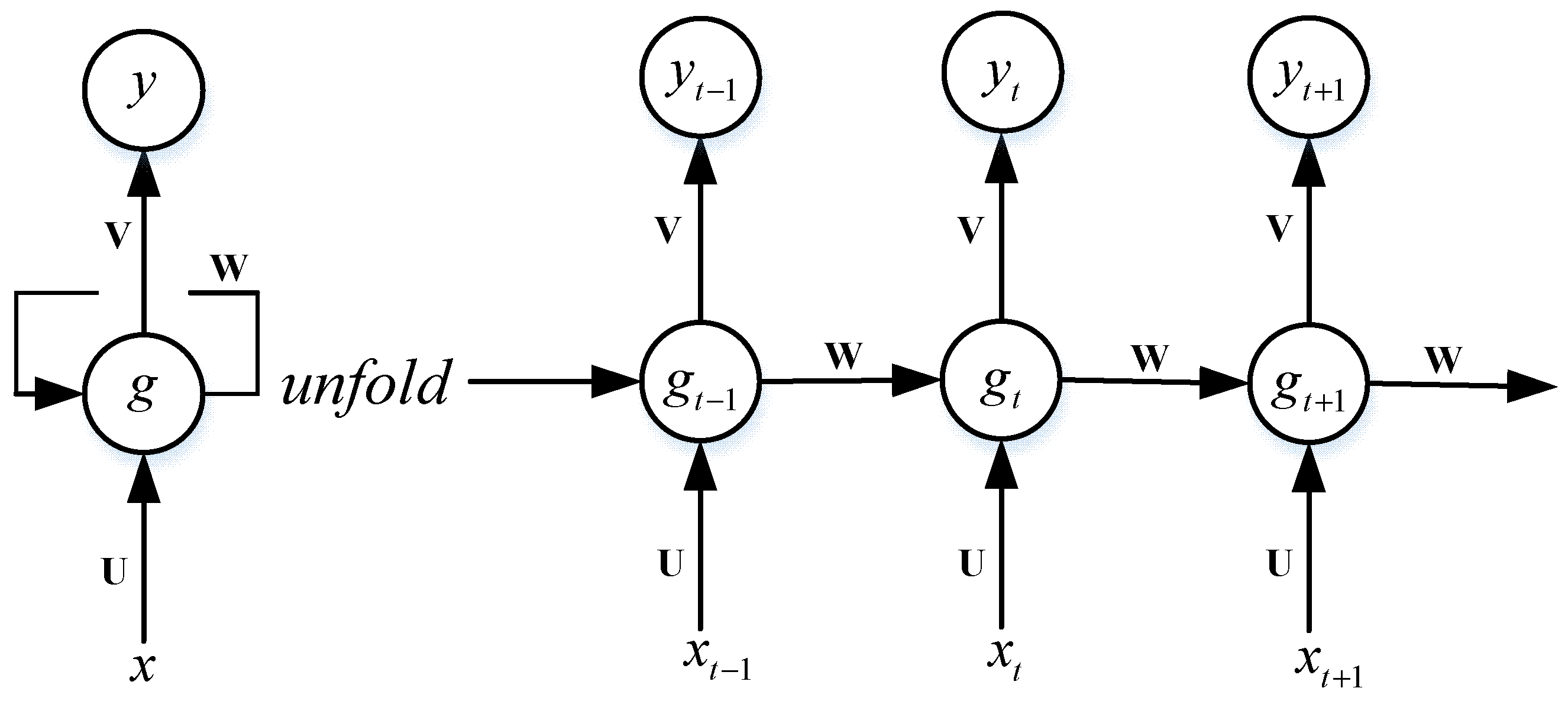
A RNN is a special kind of artificial neural network. It still consists of the input layer, the hidden layer, and the output layer [38,39]. The structure of the typical RNN model is shown in Figure 1. In the traditional feedforward NN, the nodes are connected layer by layer and there are no connections between the nodes at the same hidden layer. However, in the RNN, the nodes in the same hidden layer are connected with each other. The peculiarity is that a RNN can encode the prior information into the learning process of the current hidden layer, so the time series data can be learned efficiently. The mapping of one node can be represented as:
where represents the input at time ; is the hidden state at time , and it is also the memory unit of the network; and are the shared parameters in each layer; and represents the nonlinear function.
The connections between nodes in the RNN form a directed graph along a sequence. This allows it to exhibit dynamic temporal behavior for a time sequence. Unlike feedforward neural networks, RNNs can use their internal state (memory) to process sequences of inputs [38,39]. In theory, a RNN is suitable for predicting future values using the information from the past data. However, in practical applications, when the time interval between the previous information and the current prediction position is large, the RNN cannot memorize the previous information well, and there still exists the vanishing gradient problem, so the predicted results from the RNN are not satisfactory sometimes. In recent years, to solve this weakness and enhance the performance of the RNN, the LSTM network was proposed.
2.2. Long-Short-Term Memory Network
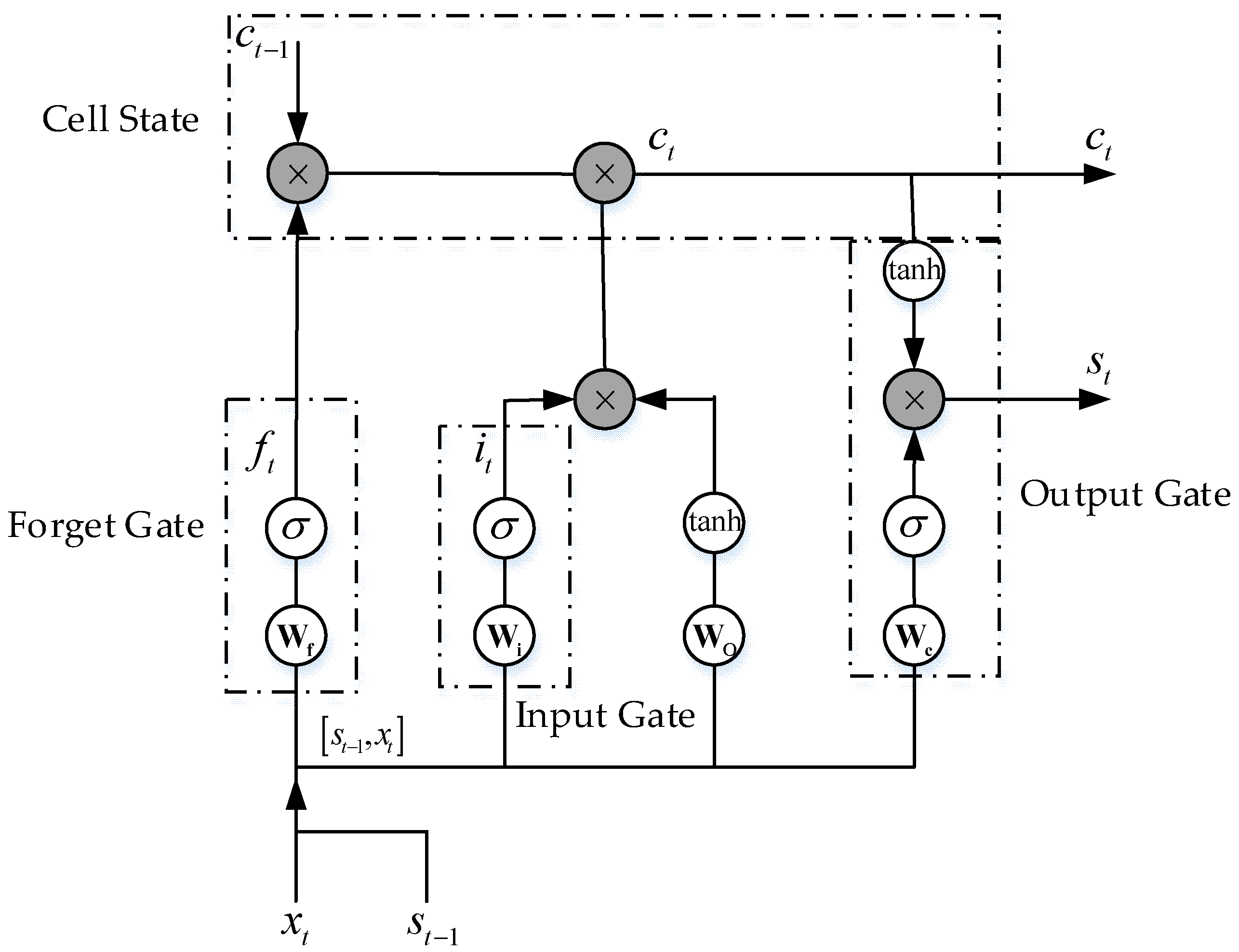
A LSTM network is a RNN which is composed of LSTM units [38,39]. The structure of the common LSTM unit is demonstrated in Figure 2. As shown in this figure, a common LSTM unit consists of a cell, an input gate, an output gate, and a forget gate. The cell is the memory in the LSTM which is used to remember the values over arbitrary time intervals. The “gate” of LSTM is a special network structure, whose input is a vector, and the output range is 0 to 1. When the output value is 0, no information is allowed to pass. When the output value is 1, all information is allowed to pass.
When the current input vector and the output vector are known, the calculation formula of the gate is expressed as follows:
where ; is the weight matrix; and is the bias vector.
In the LSTM, the role of the cell state is to record the current state. It is the core of the calculation node and can be computed as:
where is the weight matrix of the cell state; is the bias vector of the cell state; means the input gate, which determines how much of the input at the current time is saved in the cell state; and represents the forget gate used to help the network to forget the past input information and reset the memory cells. The calculation of the input gate and forget gate can be respectively expressed as:
where and are, respectively, the weight matrices of the input gate and forget gate, and and are, respectively, the bias vectors of the input gate and forget gate.
The output gate of the LSTM controls the information in the cell state of the current time to flow into the current output. The output can be expressed as:
where is the weight matrix in the output gate, and is the bias vector in the output gate.
The final output of the LSTM is computed as:
The training of the LSTM network usually adopts the back-propagation algorithm. For more details on the training and tuning of the LSTM model, please refer to [38].
2.3. Extreme Learning Machine
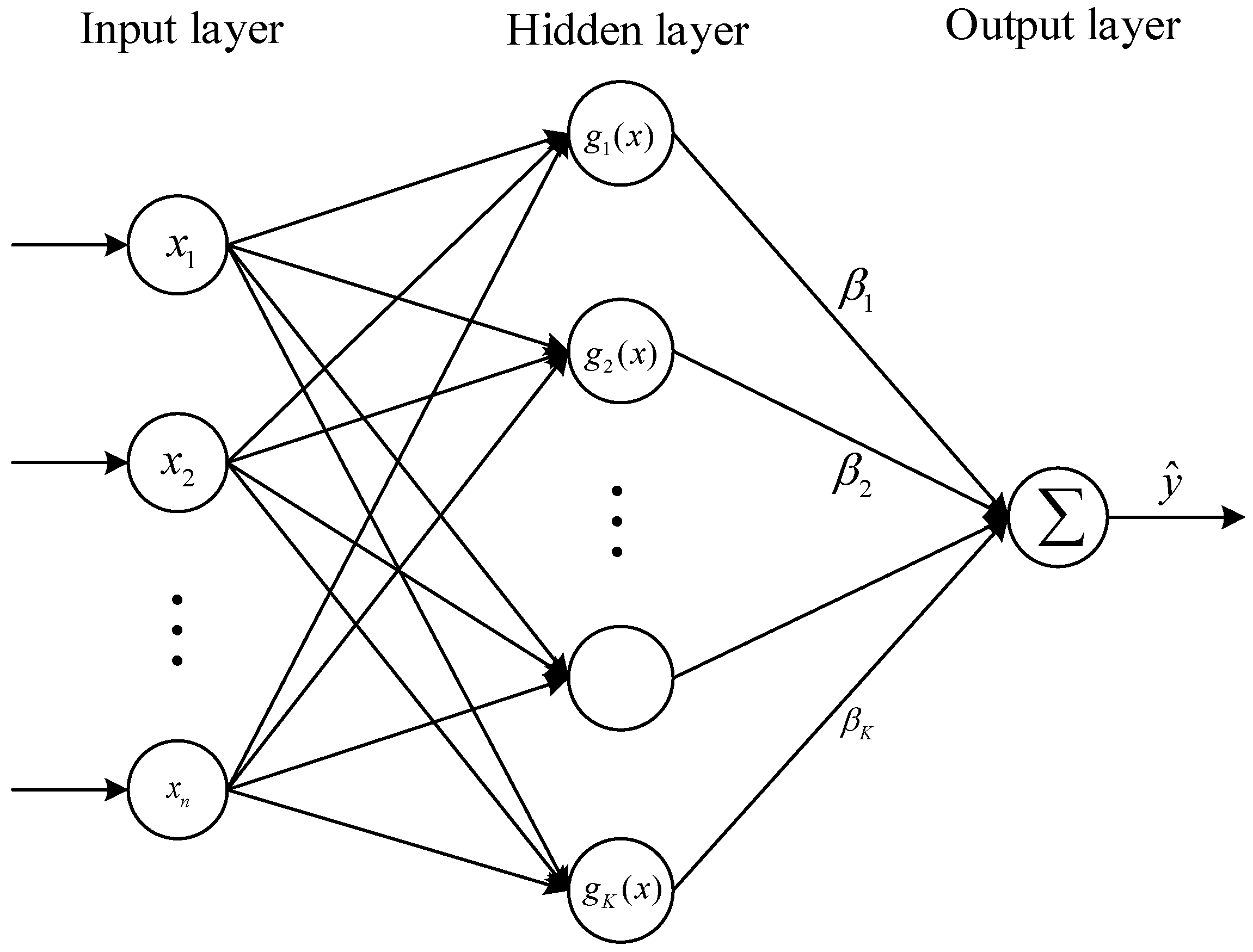
The ELM is one kind of the popular single hidden layer NNs [20]. The network structure of the ELM is shown in Figure 3. Being different from the gradient descent method (the back-propagation algorithm) commonly used in NN training process, in the ELM, its parameters before the hidden layer are randomly generated, and its weights between the hidden layer and output layer are determined by the least square method. Since there is no iterative process, the amount of calculation and the training time in the ELM can be greatly reduced. Thus, it has a very fast learning speed [20].
The input-output mapping of the ELM can be expressed as:
where represents the activation function, and:
Suppose that the training dataset is , then, the training process of the ELM can be summarized as follows [20].
Step 1: Set the number of hidden neurons and randomize the parameters in the activation functions;
Step 2: Calculate the output matrix as:
Step 3: Calculate the output weights as , where is the Moore–Penrose pseudo-inverse of the output matrix, and is the output vector and can be expressed as:
3. The Proposed Hybrid Model
In this section, the hybrid model combining the LSTM and the ELM will be proposed firstly. Then, the model evaluation indices will be presented. Finally, the data preprocessing will be introduced.
3.1. The Hybrid Model
The structure of the proposed hybrid model is demonstrated in Figure 4. As shown in this figure, once the data is input, the outputs of the LSTM model and the ELM model will be firstly calculated, then they will be ensembled by the linear regression method to generate the final output of the hybrid model.
In this hybrid model, the LSTM and ELM models can be constructed by the learning algorithms mentioned in the previous subsections. Then, to design this hybrid model, the only remaining task is to determine the parameters of the linear regression part.
Assume that, for the lth input in the aforementioned training dataset , the predicted outputs of the LSTM and ELM are, respectively, and , then we get the training dataset for the linear regression part as .
Suppose that the linear regression in the hybrid model is expressed as:
For the newly generated training dataset , we expect that:
Then, these equations can be rewritten in the matrix form as:
where:
As a result, the parameters of the linear regression part in the hybrid model can be determined as:
where is the Moore–Penrose pseudo-inverse of the matrix .
3.2. Model Evaluation Indices
In order to evaluate the performance of the proposed hybrid model, the following three indices, which are the mean absolute error (MAE), the root mean square error (RMSE), and the mean relative error (MRE), are adopted. The formulas for them can be expressed as:
where is the number of training or test samples, and are, respectively, the predicted values and real values of the electrical load.
The MAE, RMSE, and MRE are common measures of forecasting errors in time series analysis. They serve to aggregate the magnitudes of the prediction errors into a single measure. The MAE is an average of the absolute errors between the predicted values and actual observed values. In addition, the RMSE represents the sample standard deviation of the differences between the predicted values and the actual observed values. As larger errors have a disproportionately large effect on MAE and RMSE, they are sensitive to outliers. The MRE, also known as the mean absolute percentage deviation, can remedy this drawback, and it expresses the prediction accuracy as a percentage through dividing the absolute errors by their corresponding actual values. For prediction applications, the smaller the values of MAE, RMSE, and MRE, the better the forecasting performance will be.
3.3. Data Preprocessing
When the tanh function is selected as the LSTM activation function, its output value will be in the range of [–1, 1]. In order to ensure the correctness of the results from the LSTM model, the electrical load data need to be normalized in our experiments.
Suppose that the time series of the electrical load data is , then, the following equation is used to realize the normalization:
where and are, respectively, the minimum and maximum values of the electrical load data.
Then, we obtain the normalized electrical load data series as . Subsequently, this time series can be used to generate the training or testing data pairs as follows:
where in which .
4. Experiments and Comparisons
In this section, the proposed hybrid model will be applied to forecast the electrical load of the Albert area and the electrical load of one service restaurant. Detailed experiments will be conducted in these two experiments and comparisons with the LSTM, ELM, and SVR will also be made.
4.1. Electrical Load Forecasting of the Albert Area
4.1.1. Applied Dataset
The electrical load data used in this experiment was downloaded from the website of the Albert Electric System Operator (AESO) [43]. This historical electrical load dataset was collected by the Albert Electric System Operator (AESO) and provided for market participants. The electrical load data in this experiment was sampled from 1 January 2005 to 31 December 2016. Additionally, the data sampling period was one hour. This applied dataset has missing values, so, we filled in the missing values through the averaging filter to ensure the integrity and rationality of the data. Finally, this electrical load dataset contains a total of 105,192 samples. In our following experiment, the data samples from 2005 to 2015 are used for training while the data samples in 2016 are used for testing.
4.1.2. Experimental Setting
In order to determine the optimal structure of the LSTM model for the electrical load prediction, the following two design factors are considered in this paper: the number of hidden neurons and the number of input variables. The larger the number of hidden neurons, the better the modeling performance of the LSTM may be. However, with more hidden neurons, the greater the training time and the complexity of the LSTM. On the other hand, a small number of input variables will limit the prediction accuracy, while more input variables will increase the training difficulty.
In this experiment, we test five levels of the number of hidden neurons, which are 20, 40, 60, 80, and 100. Additionally, the number of the input variables is selected from eight levels, which are 5, 6, 7, 8, 9, 10, 11, and 12. Thus, 40 cases are given. Then, in each case, in order to consider the effects of the random initializations of the networks’ weights, 10 tests are run considering different random initializations. Additionally, in each case, the MAE, MRE, and RMSE are computed as the averages of those indices in the 10 runs. The averaged performances of the LSTM model in 40 cases in this experiment are shown in Table 1.
From Table 1, among all the 40 cases, the result of the 28th case is the best. That is to say, when the number of input variables is 10 and the number of hidden neurons is 60, the LSTM model can achieve the best performance. For the ELM, the number of neuron nodes is also be set to 60. The hybrid model also adopts the LSTM and ELM with the selected structure. Additionally, after being trained, the linear regression part of the hybrid model has the following expression:
Additionally, we use the software “libsvm” to realize the SVR prediction. In order to achieve as better performance as possible, the SVR is tuned by trial-and-error. The tuned SVR adopts the radial basis function as its kernel function, whose parameter gamma is set to be 0.001. The penalty coefficient of the SVR is tuned to be 100 for better performance, while the other parameters, including the loss function and the error band, are the defaults in the “libsvm”.
4.1.3. Experimental Results and Analysis
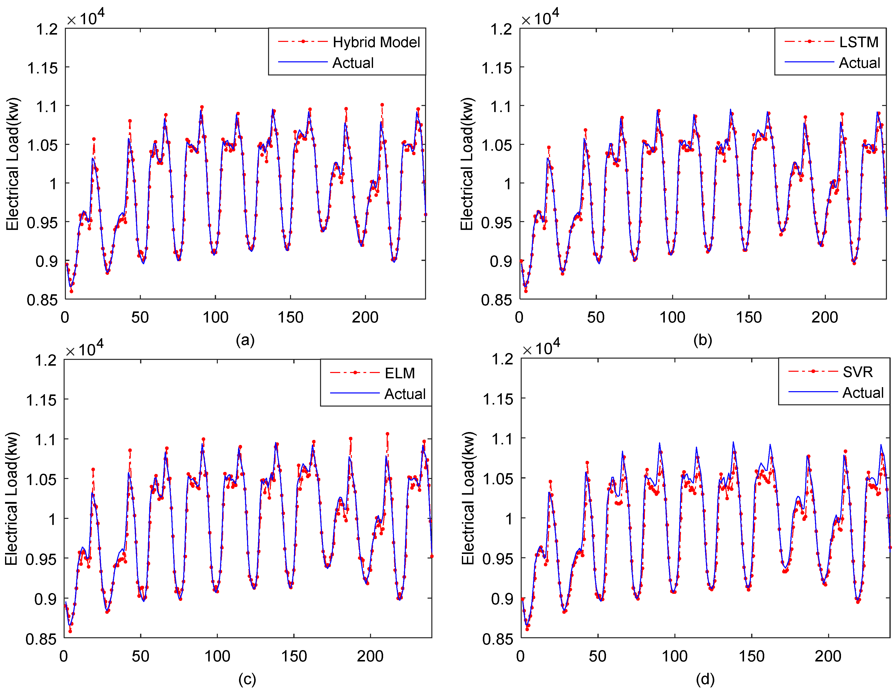
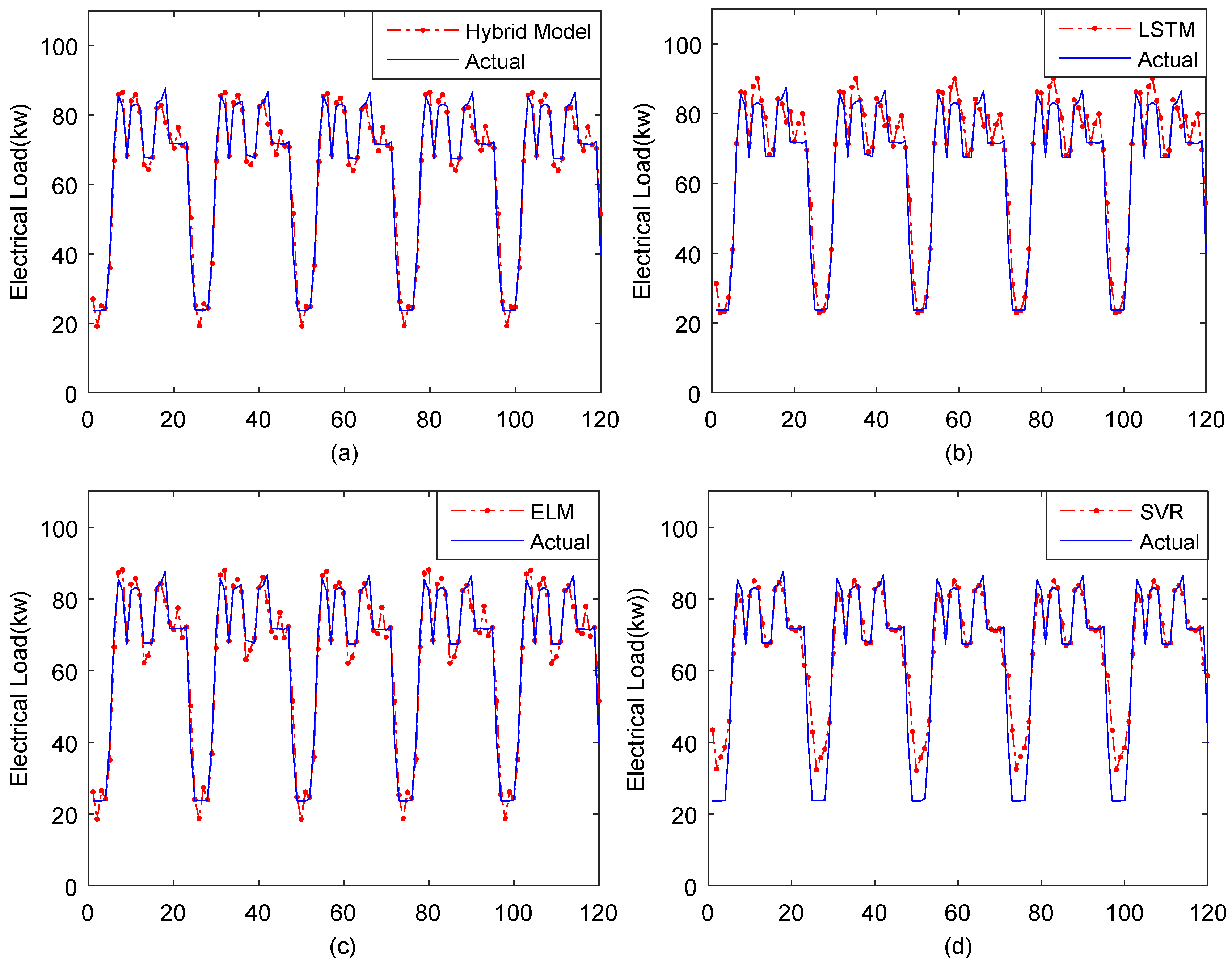
The prediction results of the four models in this application are shown in Figure 5. In order to show the details more clearly, in this figure we only plotted the prediction results of the last ten days in 2016. It can be seen from Figure 5 that the proposed hybrid model has much better performance compared with the other three models.
The performance indices of the four models are shown in Table 2. Obviously, the three indices of the proposed hybrid model are smaller than the other three models. From the point of view of these three indices, the performance of the proposed hybrid model can improve at least 5% compared to the LSTM, 8% compared to ELM, and 15% compared to SVR. In other words, in this experiment, Hybrid model > LSTM > ELM > SVR, where “>” means “performs better than”.
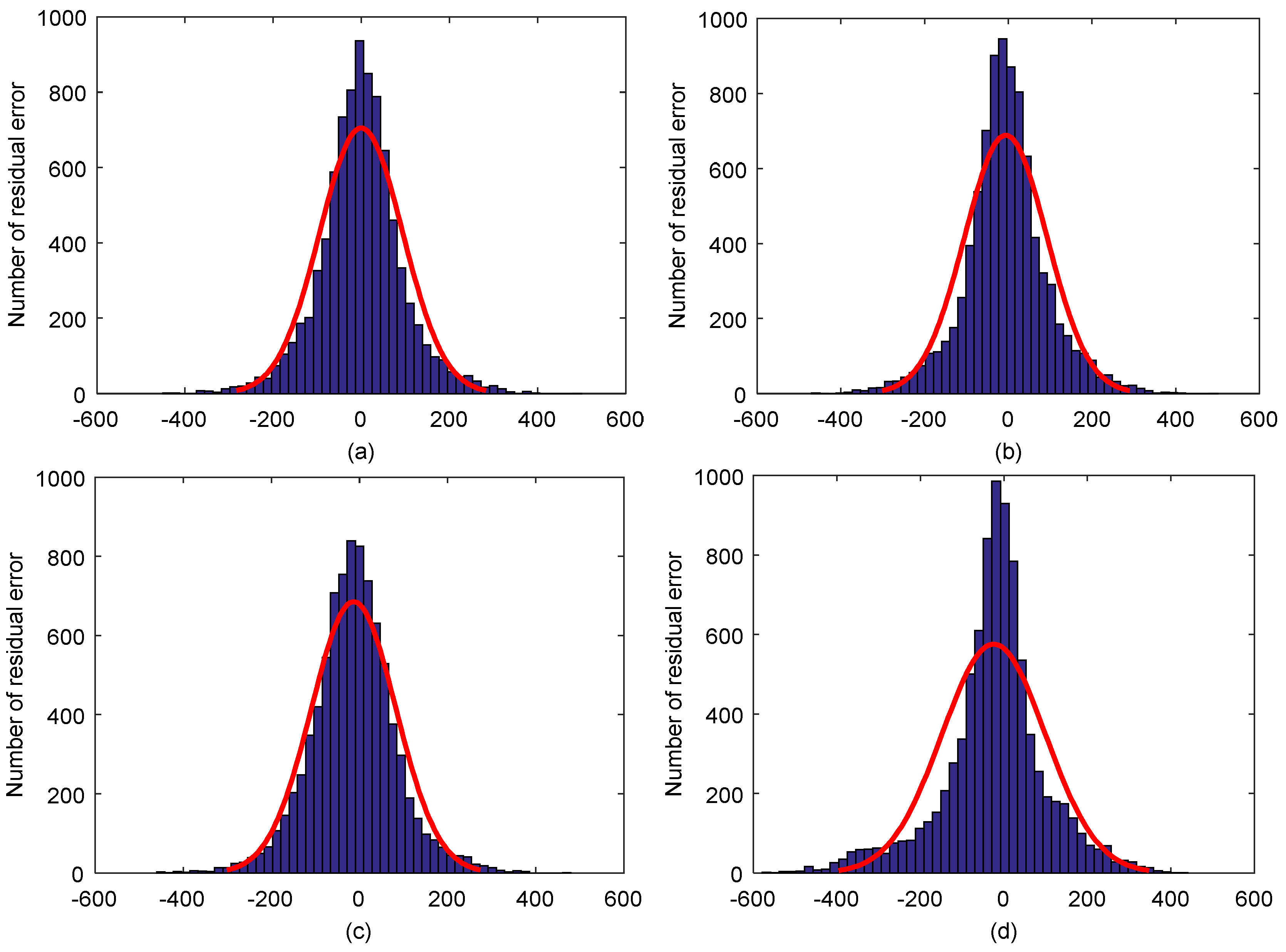
Figure 6 demonstrates the histograms of the hourly prediction errors in this experiment. Higher and narrower histogram around zero means better forecasting performance. From this figure, it is clear that the diagram of the hybrid model has much more errors locating around zero, which once again implies that the prediction performance of the proposed hybrid model is the best.
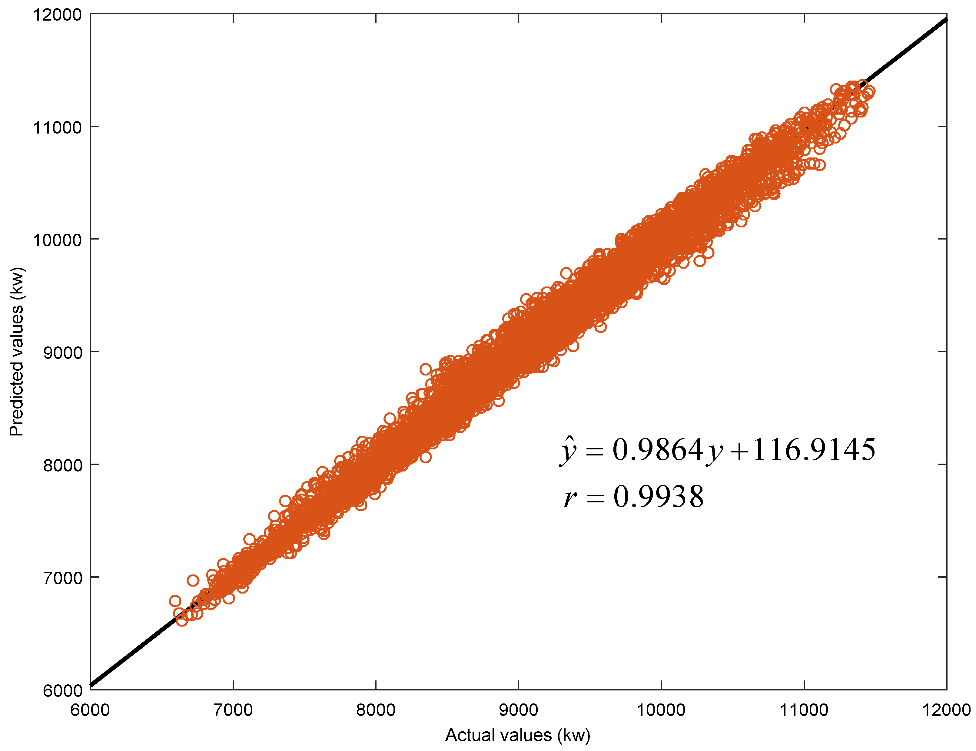
In order to better demonstrate the experimental performance of the proposed hybrid model, the scatter plots of the actual and predicted values of the electrical load in the first experiment are drawn in Figure 7. This figure also verifies that the proposed hybrid model can provide satisfied fitting performance.
4.2. Electrical Load Forecasting of One Service Restaurant
4.2.1. Applied Dataset
The electrical load dataset in the second experiment was downloaded from [44]. This dataset contains hourly load profile data for 16 commercial building types and residential buildings in the United States. In this study, we select the electrical load data of one service restaurant in Helena, MT, USA for our experiment. The selected time series data were collected from 1 January 2004 to 31 December 2004 with an hourly sampling period. Again, in this experiment, we apply the averaging filter to fill in the missing values. Hence, in total, we have 8760 samples. In our experiment, the data in the first ten months are chosen for training and the ones in the last two months are for testing.
4.2.2. Experimental Setting
The method for determining the optimal structure of the LSTM model is similar to that in the first experiment. In this application, the number of hidden neurons is also chosen from the same five levels, while the number of the input variables is tested among the same eight levels. As a result, there still exist 40 cases in this experiment. Again, in each case, 10 different random initializations are considered. The averaged indices of the LSTM model in 40 cases in this application are shown in Table 3.
From this table, we can observe that case 35 has the best performance. In other words, the optimal structure of the LSTM model has 12 input variables and 100 neurons in the hidden layer. Similarly, the number of hidden neurons in the ELM is set to be 100. Further, the hybrid model is constructed by ensembling these two LSTM and ELM models. The regression part for this ensembling is obtained after learning as follows:
Additionally, for the SVR in this application, we also use the radial basis function as the kernel function, but the parameter gamma is tuned to be 0.1, and the penalty coefficient is tuned to be 110. Again, the defaults in the “libsvm” are used for the other parameters, including the loss function and the error band in this application.
4.2.3. Experimental Results and Analysis
For the testing data, the forecasting results of the last five days from the four models are demonstrated in Figure 8. Additionally, in order to show the improvement of the proposed hybrid model, the performance indices of the four models in this application are listed in Table 4. From Figure 8 and Table 4, we once again observe that the proposed hybrid model can achieve the best performance in this electrical load forecasting application. Compared with the other three comparative methods, the improvement of the proposed hybrid model can achieve at least 33.3%, 31.6%, and 52.5% according to the indices MAE, MRE, and RMSE, respectively.
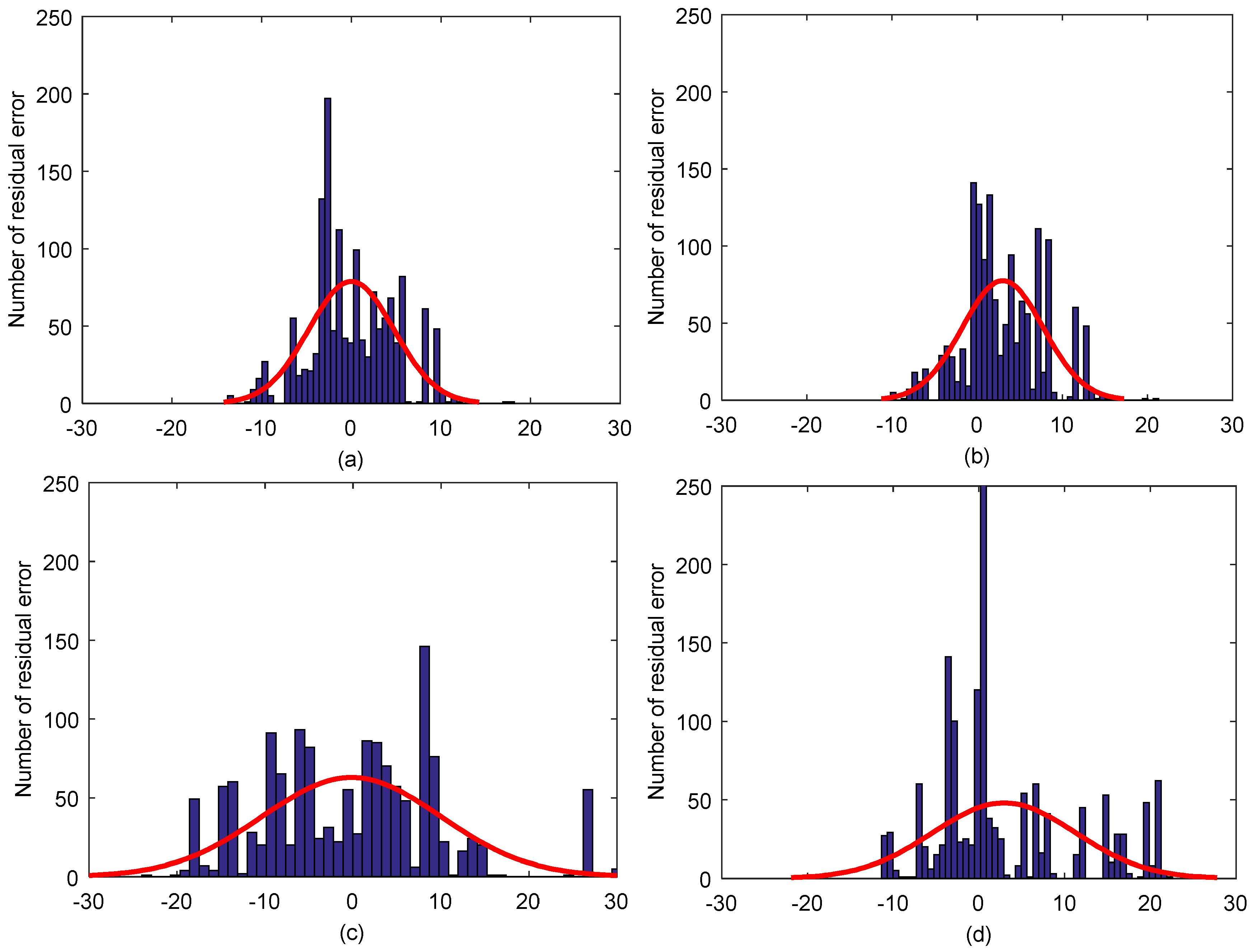
To further reflect the differences of the four methods, the histograms of their prediction errors in this application are demonstrated in Figure 9. From Figure 9a, we can observe that the mean of the forecasting errors of the proposed hybrid model is located around zero, which implies that the forecasting errors of the proposed hybrid model are relatively small. From Figure 9b, it can be seen that the center of the forecasting errors of the LSTM model is greater than zero. This means that the LSTM model has larger prediction errors than the hybrid model. Comparing Figure 9c,d with Figure 9a, we can find that the error histograms of the ELM and SVR are lower and fatter than that of the proposed hybrid model. Just as mentioned previously, the lower and flatter error histogram means the worse performance. We can also observe from Figure 9d that some forecasting errors of the SVR are very large. Overall, in this electrical load forecasting application, the hybrid model > LSTM > ELM > SVR again.
5. Conclusions
The short-term electrical load forecasting plays an important role in the efficient management of the power grid. This study presented one hybrid model for the short-term electrical load forecasting. The proposed hybrid model used the ELM method to model the shallow features of the electrical load and adopted the LSTM method to extract the deep patterns. In the hybrid model, the predicted results from the ELM and LSTM are ensembled by one linear regression which is determined by the least square method. Two real-world electrical load forecasting applications were also given to evaluate the performance of the proposed hybrid model. Experimental results demonstrated that the proposed hybrid model can give satisfactory prediction accuracy and can achieve the best results compared with the comparative methods. The experimental results also indicate that the LSTM can use its memory cells to learn and retain useful information in the historical data of electrical load for a long period of time, and use its forget gates to remove useless information, which makes the hybrid model have excellent learning performance and generalization ability. The proposed hybrid method can also be applied to some other time series prediction problems, e.g., building energy consumption prediction and traffic flow estimates.
However, in this study, our work only used the linear regression to ensemble the LSTM and the ELM. As the non-linear function may be better to accommodate the eventual nonlinearities when ensembling the LSTM and ELM, in our near-future study we will select appropriate non-linear functions to realize the ensembling. On the other hand, our work only attempts to use the data to realize the electrical load prediction without considering any practical information for electricity consumption-related principles. Our future study will also attempt to consider the electricity consumption-related principles to further improve the forecasting precision of the short-term electrical load.
Author Contributions
Chengdong Li and Guiqing Zhang have contributed to developing ideas about the hybrid prediction method and collecting the data. Liwen Xu and Xiuying Xie programmed the algorithm and tested it. All of the authors were involved in preparing the manuscript.
Acknowledgments
This work is supported by National Natural Science Foundation of China (61473176, 61105077, 61573225), the Natural Science Foundation of Shandong Province for Young Talents in Province Universities (ZR2015JL021), and the Taishan Scholar Project of Shandong Province of China (2015162).
Conflicts of Interest
The authors declare no conflict of interest.
References
- Global Power Report. Available online: http://www.powerchina.cn/art/2016/9/20/art_26_186950.html (accessed on 5 May 2018).
- Pappas, S.S.; Ekonomou, L.; Karamousantas, D.C.; Chatzarakis, G.E. Electricity demand loads modeling using AutoRegressive Moving Average (ARMA) models. Energy 2008, 33, 1353–1360. [Google Scholar] [CrossRef]
- Im, K.M.; Lim, J.H. A design of short-term load forecasting structure based on ARIMA using load pattern classification. Commun. Comput. Inf. Sci. 2011, 185, 296–303. [Google Scholar]
- Huang, S.J.; Shih, K.R. Short-term load forecasting via ARMA model identification including non-Gaussian process considerations. IEEE Trans. Power Syst. 2003, 18, 673–679. [Google Scholar] [CrossRef]
- Papalexopoulos, A.D.; Hesterberg, T.C. A regression-based approach to short-term system load forecasting. IEEE Trans. Power Syst. 1990, 5, 1535–1547. [Google Scholar] [CrossRef]
- Hong, T.; Gui, M.; Baran, M.E.; Willis, H.L. Modeling and forecasting hourly electric load by multiple linear regression with interactions. In Proceedings of the IEEE Power and Energy Society General Meeting, Providence, RI, USA, 25–29 July 2010; pp. 1–8. [Google Scholar]
- Vamvakas, P.; Tsiropoulou, E.E.; Papavassiliou, S. Dynamic provider selection & power resource management in competitive wireless communication markets. Mob. Netw. Appl. 2017, 7, 1–14. [Google Scholar]
- Tsiropoulou, E.E.; Katsinis, G.K.; Filios, A.; Papavassiliou, S. On the problem of optimal cell selection and uplink power control in open access multi-service two-tier femtocell networks. In Proceedings of the International Conference on Ad-Hoc Networks and Wireless, Benidorm, Spain, 22–27 June 2014; pp. 114–127. [Google Scholar]
- Cordeschi, N.; Amendola, D.; Shojafar, M.; Baccarelli, E. Performance evaluation of primary-secondary reliable resource-management in vehicular networks. In Proceedings of the IEEE 25th Annual International Symposium on Personal, Indoor, and Mobile Radio Communication, Washington, DC, USA, 2–5 September 2014; pp. 959–964. [Google Scholar]
- Cordeschi, N.; Amendola, D.; Shojafar, M.; Naranjo, P.G.V.; Baccarelli, E. Memory and memoryless optimal time-window controllers for secondary users in vehicular networks. In Proceedings of the International Symposium on Performance Evaluation of Computer and Telecommunication Systems, Chicago, IL, USA, 26–29 July 2015; pp. 1–7. [Google Scholar]
- Espinoza, M. Fixed-size least squares support vector machines: A large scale application in electrical load forecasting. Comput. Manag. Sci. 2006, 3, 113–129. [Google Scholar] [CrossRef]
- Chen, Y.B.; Xu, P.; Chu, Y.Y.; Li, W.L.; Wu, Y.T.; Ni, L.Z.; Bao, Y.; Wang, K. Short-term electrical load forecasting using the Support Vector Regression (SVR) model to calculate the demand response baseline for office buildings. Appl. Energy 2017, 195, 659–670. [Google Scholar] [CrossRef]
- Duan, P.; Xie, K.G.; Guo, T. T.; Huang, X.G. Short-term load forecasting for electric power systems using the PSO-SVR and FCM clustering techniques. Energies 2011, 4, 173–184. [Google Scholar] [CrossRef]
- Agarwal, V.; Bougaev, A.; Tsoukalas, L. Kernel regression based short-term load forecasting. In Proceedings of the International Conference on Artificial Neural Networks, Athens, Greece, 10–14 September 2006; pp. 701–708. [Google Scholar]
- Mordjaoui, M.; Haddad, S.; Medoued, A.; Laouafi, A. Electric load forecasting by using dynamic neural network. Int. J. Hydrog. Energy 2017, 28, 17655–17663. [Google Scholar] [CrossRef]
- Pan, L.N.; Feng, X.S.; Sang, F.W.; Li, L.J.; Leng, M.W. An improved back propagation neural network based on complexity decomposition technology and modified flower pollination optimization for short-term load forecasting. Neural Comput. Appl. 2017, 13, 1–19. [Google Scholar] [CrossRef]
- Leme, R.C.; Souza, A.C.Z.D.; Moreira, E.M.; Pinheiro, C.A.M. A hierarchical neural model with time windows in long-term electrical load forecasting. Neural Comput. Appl. 2006, 16, 456–470. [Google Scholar]
- Li, H.Z.; Guo, S.; Li, C.J.; Sun, J.Q. A hybrid annual power load forecasting model based on generalized regression neural network with fruit fly optimization algorithm. Knowl. Based Syst. 2013, 37, 378–387. [Google Scholar] [CrossRef]
- Salkuti, S.R. Short-term electrical load forecasting using radial basis function neural networks considering weather factors. Electri. Eng. 2018, 5, 1–11. [Google Scholar] [CrossRef]
- Huang, G.B.; Zhu, Q.Y.; Siew, C.K. Extreme learning machine: A new learning scheme of feedforward neural networks. In Proceedings of the IEEE International Joint Conference on Neural Networks, Budapest, Hungary, 25–29 July 2004; pp. 985–990. [Google Scholar]
- Zhu, Q.Y.; Qin, A.K.; Suganthan, P.N.; Huang, G.B. Rapid and brief communication: Evolutionary extreme learning machine. Pattern Recognit. 2005, 38, 1759–1763. [Google Scholar] [CrossRef]
- Ertugrul, O.F. Forecasting electricity load by a novel recurrent extreme learning machines approach. Int. J. Electr. Power Energy Syst. 2016, 78, 429–435. [Google Scholar] [CrossRef]
- Zhang, R.; Dong, Z.Y.; Xu, Y.; Meng, K.; Wong, K.P. Short-term load forecasting of Australian National Electricity Market by an ensemble model of extreme learning machine. IET Gener. Transm. Dis. 2013, 7, 391–397. [Google Scholar] [CrossRef]
- Kaelbling, L.P.; Littman, M.L.; Moore, A.W. Reinforcement learning: A survey. J. Artifi. Intell. Res. 1996, 4, 237–285. [Google Scholar]
- Boyan, J.A. Generalization in reinforcement learning: Safely approximating the value function. In Proceedings of the Neural Information Processings Systems, Denver, CO, USA, 27 November–2 December 1995; pp. 369–376. [Google Scholar]
- Xiong, R.; Cao, J.; Yu, Q. Reinforcement learning-based real-time power management for hybrid energy storage system in the plug-in hybrid electric vehicle. Appl. Energy 2018, 211, 538–548. [Google Scholar] [CrossRef]
- Li, C.D.; Ding, Z.X.; Zhao, D.B.; Yi, J.Q.; Zhang, G.Q. Building energy consumption prediction: An extreme deep learning approach. Energies 2017, 10, 1525. [Google Scholar] [CrossRef]
- Li, C.D.; Ding, Z.X.; Yi, J.Q.; Lv, Y.S.; Zhang, G.Q. Deep belief network based hybrid model for building energy consumption prediction. Energies 2018, 11, 242. [Google Scholar] [CrossRef]
- Dong, Y.; Liu, Y.; Lian, S.G. Automatic age estimation based on deep learning algorithm. Neurocomputing 2016, 187, 4–10. [Google Scholar] [CrossRef]
- Raveane, W.; Arrieta, M.A.G. Shared map convolutional neural networks for real-time mobile image recognition. In Distributed Computing and Artificial Intelligence, 11th International Conference; Springer International Publishing: Cham, Switzerland, 2014; pp. 485–492. [Google Scholar]
- Kumaran, N.; Vadivel, A.; Kumar, S.S. Recognition of human actions using CNN-GWO: A novel modeling of CNN for enhancement of classification performance. Multimed. Tools Appl. 2018, 1, 1–33. [Google Scholar] [CrossRef]
- Potluri, S.; Fasih, A.; Vutukuru, L.K.; Machot, F.A.; Kyamakya, K. CNN based high performance computing for real time image processing on GPU. In Proceedings of the Joint INDS'11 & ISTET'11, Klagenfurt, Austria, 25–27 July 2011; pp. 1–7. [Google Scholar]
- Ahmad, J.; Sajjad, M.; Rho, S.; Kwon, S.I.; Lee, M.Y.; Balk, S.W. Determining speaker attributes from stress-affected speech in emergency situations with hybrid SVM-DNN architecture. Multimed. Tools Appl. 2016, 1–25. [Google Scholar] [CrossRef]
- Wu, Z.Y.; Zhao, K.; Wu, X.X.; Lan, X.Y.; Meng, L. Acoustic to articulatory mapping with deep neural network. Multimed. Tools Appl. 2015, 74, 9889–9907. [Google Scholar] [CrossRef]
- Lv, Y.S.; Duan, Y.J.; Kang, W.W.; Li, Z.X.; Wang, F.Y. Traffic flow prediction with big data: A deep learning approach. IEEE T. Intell. Transp. Syst. 2015, 16, 865–873. [Google Scholar] [CrossRef]
- Ma, X.L.; Yu, H.Y.; Wang, Y.P.; Wang, Y.H. Large-scale transportation network congestion evolution prediction using deep learning theory. Plos One 2015, 10. [Google Scholar] [CrossRef] [PubMed]
- Yu, D.H.; Liu, Y.; Yu, X. A data grouping CNN algorithm for short-term traffic flow forecasting. In Asia-Pacific Web Conference; Springer: Cham, Switzerland, 2016; pp. 92–103. [Google Scholar]
- Hochreiter, S.; Schmidhuber, J. Long short-term memory. Neural Comput. 1997, 9, 1735–1780. [Google Scholar] [CrossRef] [PubMed]
- Che, Z.; Purushotham, S.; Cho, K.; Sontag, D.; Liu, Y. Recurrent neural networks for multivariate time series with missing values. Sci. Rep. 2018, 8, 6085. [Google Scholar] [CrossRef] [PubMed]
- Lipton, Z.C.; Kale, D.C.; Wetzel, R. Modeling Missing Data in Clinical Time Series with RNNs. Available online: http://proceedings.mlr.press/v56/Lipton16.pdf (accessed on 5 July 2018).
- Ma, X.; Tao, Z.; Wang, Y.; Yu, H.; Wang, Y. Long short-term memory neural network for traffic speed prediction using remote microwave sensor data. Transp. Res. Part C 2015, 54, 187–197. [Google Scholar] [CrossRef]
- Karim, F.; Majumdar, S.; Darabi, H.; Chen, S. LSTM fully convolutional networks for time series classification. IEEE Access 2018, 6, 1662–1669. [Google Scholar] [CrossRef]
- AESO Electrical Load Data Set. Available online: https://www.aeso.ca. (accessed on 12 March 2018).
- Commercial and Residential Buildings’ Hourly Load Dataset. Available online: https://openei.org/datasets/dataset/commercial-and-residential-hourly-load-profiles-for-all-tmy3-locations-in-the-united-states. (accessed on 13 April 2018).
Figure 1.
The structure of the typical RNN model.

Figure 2.
The structure of the LSTM unit.

Figure 3.
The structure of the ELM.

Figure 4.
The structure of the proposed hybrid model.

Figure 5.
Experimental results of the last ten days in 2016 in the first experiment: (a) Hybrid model; (b) LSTM, (c) ELM; (d) SVR.
Figure 5.
Experimental results of the last ten days in 2016 in the first experiment: (a) Hybrid model; (b) LSTM, (c) ELM; (d) SVR.

Figure 6.
Histograms of the hourly prediction errors in the first experiment: (a) Hybrid model; (b) LSTM; (c) ELM; and (d) SVR.
Figure 6.
Histograms of the hourly prediction errors in the first experiment: (a) Hybrid model; (b) LSTM; (c) ELM; and (d) SVR.

Figure 7.
The actual and predicted values of the electrical load in the first experiment.

Figure 8.
Experimental results of the last five days in the second application: (a) Hybrid model; (b) LSTM; (c) ELM; and (d) SVR.
Figure 8.
Experimental results of the last five days in the second application: (a) Hybrid model; (b) LSTM; (c) ELM; and (d) SVR.

Figure 9.
Histograms of the prediction errors in thesecond experiment, (a) Hybrid model; (b) LSTM; (c) ELM; and (d) SVR.
Figure 9.
Histograms of the prediction errors in thesecond experiment, (a) Hybrid model; (b) LSTM; (c) ELM; and (d) SVR.


Table 1.
The averaged performances of the LSTM model in 40 cases in the first experiment.
| Trial | Input | Cell | Averaged Indices | Trial | Input | Cell | Averaged Indices | ||||
|---|---|---|---|---|---|---|---|---|---|---|---|
| MAE | MRE(%) | RMSE | MAE | MRE(%) | RMSE | ||||||
| 1 | 5 | 20 | 116.9954 | 1.2601 | 152.1007 | 21 | 9 | 20 | 102.1704 | 1.0997 | 132.9284 |
| 2 | 5 | 40 | 97.2733 | 1.0570 | 129.7889 | 22 | 9 | 40 | 122.0178 | 1.3104 | 151.9188 |
| 3 | 5 | 60 | 84.5351 | 0.9317 | 116.7891 | 23 | 9 | 60 | 95.1910 | 1.0435 | 122.9191 |
| 4 | 5 | 80 | 89.2817 | 0.9798 | 121.4982 | 24 | 9 | 80 | 80.6772 | 0.8834 | 108.8855 |
| 5 | 5 | 100 | 86.1510 | 0.9516 | 117.5446 | 25 | 9 | 100 | 90.6934 | 0.9839 | 122.7209 |
| 6 | 6 | 20 | 84.5489 | 0.9283 | 116.2049 | 26 | 10 | 20 | 98.7483 | 1.0667 | 127.0956 |
| 7 | 6 | 40 | 85.0707 | 0.9425 | 117.9868 | 27 | 10 | 40 | 91.7649 | 0.9960 | 119.4111 |
| 8 | 6 | 60 | 97.7385 | 1.0591 | 129.7166 | 28 | 10 | 60 | 72.2753 | 0.7963 | 98.4589 |
| 9 | 6 | 80 | 115.2194 | 1.2475 | 146.6029 | 29 | 10 | 80 | 73.5594 | 0.8078 | 99.5021 |
| 10 | 6 | 100 | 84.7226 | 0.9298 | 118.0570 | 30 | 10 | 100 | 82.0465 | 0.8944 | 109.2512 |
| 11 | 7 | 20 | 91.4179 | 1.0080 | 120.6575 | 31 | 11 | 20 | 73.3172 | 0.8060 | 98.6403 |
| 12 | 7 | 40 | 82.4949 | 0.9090 | 112.7130 | 32 | 11 | 40 | 76.3391 | 0.8406 | 102.6357 |
| 13 | 7 | 60 | 86.2502 | 0.9427 | 116.7535 | 33 | 11 | 60 | 79.0162 | 0.8680 | 104.7912 |
| 14 | 7 | 80 | 98.2174 | 1.0788 | 126.8882 | 34 | 11 | 80 | 85.3047 | 0.9272 | 112.1438 |
| 15 | 7 | 100 | 82.4535 | 0.9047 | 114.1381 | 35 | 11 | 100 | 105.8272 | 1.1464 | 132.3876 |
| 16 | 8 | 20 | 125.2901 | 1.3474 | 161.0009 | 36 | 12 | 20 | 77.5761 | 0.8551 | 102.5785 |
| 17 | 8 | 40 | 81.4138 | 0.8948 | 110.8346 | 37 | 12 | 40 | 93.2179 | 1.0102 | 120.6827 |
| 18 | 8 | 60 | 84.5120 | 0.9297 | 114.3067 | 38 | 12 | 60 | 81.2607 | 0.8938 | 106.8901 |
| 19 | 8 | 80 | 106.8368 | 1.1719 | 138.6301 | 39 | 12 | 80 | 128.2620 | 1.3791 | 160.0733 |
| 20 | 8 | 100 | 113.2714 | 1.2239 | 144.1222 | 40 | 12 | 100 | 124.7561 | 1.3343 | 163.9346 |
Table 2.
The performance indices of the four models in the first experiment.
| MAE | MRE(%) | RMSE | |
|---|---|---|---|
| Hybrid model | 68.7121 | 0.7565 | 93.2667 |
| LSTM | 72.0921 | 0.7924 | 98.6150 |
| ELM | 85.2096 | 0.9272 | 121.0129 |
| SVR | 81.3732 | 0.8884 | 115.8054 |
Table 3.
The averaged indices of the LSTM model in the second experiment.
| Trial | Input | Cell | Averaged Indices | Trial | Input | Cell | Averaged iIndices | ||||
|---|---|---|---|---|---|---|---|---|---|---|---|
| MAE | MRE(%) | RMSE | MAE | MRE(%) | RMSE | ||||||
| 1 | 6 | 20 | 7.1771 | 12.9736 | 9.6727 | 21 | 10 | 20 | 7.7198 | 13.9318 | 9.9992 |
| 2 | 6 | 40 | 6.2598 | 12.5989 | 9.3245 | 22 | 10 | 40 | 7.0582 | 13.0492 | 9.6955 |
| 3 | 6 | 60 | 5.5457 | 10.8710 | 8.3062 | 23 | 10 | 60 | 5.5835 | 10.0200 | 8.0960 |
| 4 | 6 | 80 | 5.5134 | 10.6229 | 8.2383 | 24 | 10 | 80 | 6.4581 | 11.5403 | 9.0721 |
| 5 | 6 | 100 | 7.1821 | 12.4820 | 9.3755 | 25 | 10 | 100 | 5.9818 | 11.0428 | 8.6531 |
| 6 | 7 | 20 | 7.5924 | 14.3682 | 9.9352 | 26 | 11 | 20 | 7.0673 | 13.5552 | 9.7034 |
| 7 | 7 | 40 | 6.6790 | 13.1658 | 8.9878 | 27 | 11 | 40 | 6.6684 | 12.7804 | 9.4788 |
| 8 | 7 | 60 | 6.6408 | 13.2102 | 9.2235 | 28 | 11 | 60 | 6.8561 | 13.5773 | 9.3759 |
| 9 | 7 | 80 | 6.5768 | 12.0001 | 8.7904 | 29 | 11 | 80 | 4.8765 | 8.8409 | 7.1536 |
| 10 | 7 | 100 | 6.2907 | 11.0141 | 8.4172 | 30 | 11 | 100 | 5.2019 | 9.4162 | 6.9256 |
| 11 | 8 | 20 | 7.1725 | 14.1086 | 9.9249 | 31 | 12 | 20 | 6.9364 | 12.7357 | 9.1828 |
| 12 | 8 | 40 | 7.7985 | 15.1546 | 10.3129 | 32 | 12 | 40 | 6.9170 | 12.7038 | 9.1602 |
| 13 | 8 | 60 | 7.1521 | 13.3672 | 9.8928 | 33 | 12 | 60 | 7.5057 | 13.7293 | 9.5874 |
| 14 | 8 | 80 | 6.9347 | 14.0792 | 9.9348 | 34 | 12 | 80 | 5.2464 | 10.3753 | 7.2903 |
| 15 | 8 | 100 | 6.0706 | 11.9748 | 8.6654 | 35 | 12 | 100 | 4.2324 | 7.9345 | 5.7119 |
| 16 | 9 | 20 | 6.3518 | 12.7758 | 9.3983 | 36 | 13 | 20 | 6.3514 | 12.7800 | 8.8737 |
| 17 | 9 | 40 | 7.3086 | 14.3657 | 9.7797 | 37 | 13 | 40 | 6.3419 | 12.4733 | 9.0717 |
| 18 | 9 | 60 | 6.4742 | 12.0802 | 9.2994 | 38 | 13 | 60 | 5.3390 | 10.7757 | 7.1112 |
| 19 | 9 | 80 | 5.7523 | 11.1158 | 8.2278 | 39 | 13 | 80 | 5.2022 | 10.2410 | 6.5495 |
| 20 | 9 | 100 | 5.9189 | 10.8050 | 8.2184 | 40 | 13 | 100 | 5.3477 | 10.8264 | 6.9637 |
Table 4.
The performance indices of the four models in the second experiment.
| MAE | MRE(%) | RMSE | |
| Hybrid Model | 2.8782 | 5.4335 | 3.6224 |
| LSTM | 4.2631 | 7.9125 | 5.6178 |
| ELM | 5.7569 | 10.5350 | 6.7282 |
| SVR | 5.9182 | 16.7053 | 8.5685 |
© 2018 by the authors. Licensee MDPI, Basel, Switzerland. This article is an open access article distributed under the terms and conditions of the Creative Commons Attribution (CC BY) license (http://creativecommons.org/licenses/by/4.0/).
Share and Cite
MDPI and ACS Style
Xu, L.; Li, C.; Xie, X.; Zhang, G. Long-Short-Term Memory Network Based Hybrid Model for Short-Term Electrical Load Forecasting. Information 2018, 9, 165. https://doi.org/10.3390/info9070165
AMA Style
Xu L, Li C, Xie X, Zhang G. Long-Short-Term Memory Network Based Hybrid Model for Short-Term Electrical Load Forecasting. Information. 2018; 9(7):165. https://doi.org/10.3390/info9070165
Chicago/Turabian StyleXu, Liwen, Chengdong Li, Xiuying Xie, and Guiqing Zhang. 2018. "Long-Short-Term Memory Network Based Hybrid Model for Short-Term Electrical Load Forecasting" Information 9, no. 7: 165. https://doi.org/10.3390/info9070165
Note that from the first issue of 2016, this journal uses article numbers instead of page numbers. See further details here.