Aerial-Image Denoising Based on Convolutional Neural Network with Multi-Scale Residual Learning Approach

Abstract

Aerial images are subject to various types of noise, which restricts the recognition and analysis of images, target monitoring, and search services. At present, deep learning is successful in image recognition. However, traditional convolutional neural networks (CNNs) extract the main features of an image to predict directly and are limited by the requirements of the training sample size (i.e., a small data size is not successful enough). In this paper, using a small sample size, we propose an aerial-image denoising recognition model based on CNNs with a multi-scale residual learning approach. The proposed model has the following three advantages: (1) Instead of directly learning latent clean images, the proposed model learns the noise from noisy images and then subtracts the learned residual from the noisy images to obtain reconstructed (denoised) images; (2) The developed image denoising recognition model is beneficial to small training datasets; (3) We use multi-scale residual learning as a learning approach, and dropout is introduced into the model architecture to force the network to learn to generalize well enough. Our experimental results on aerial-image denoising recognition reveal that the proposed approach is highly superior to the other state-of-the-art methods.

1. Introduction

As one of the classical problems in aerial imaging, aerial images for regional scenes, searching, and military scouting are subject to various types and degrees of noise, which may occur during transmission and acquisition. The appearance of noise in aerial images interferes with the quality of the original images, which has direct or indirect influences that complicate the timely recognition, analysis, target monitoring, and search services [1]. Therefore, image denoising is a crucial issue in the field of computer vision that has been widely discussed and studied by researchers [2,3,4]. At present, most of the existing denoising methods mainly focus on the scenario of additive white Gaussian noise (AWGN), whereby an observed noisy image $y$ is modeled as a combination of a clean image $x$ and AWGN $v$; that is, $y=x+v$. Using a general model, Elad & Aharon [5] presented sparse and redundant representations over learned dictionaries, whereby the proposed algorithm simultaneously trained a dictionary on its content using the K-SVD algorithm. However, its computational complexity is one of the shortcomings of this algorithm.

In recent years, with the development of deep learning, the research results of deep architecture have shown good performance [6,7,8,9]. In the task of image denoising, Frost et al. [10] and Kuan et al. [11] proposed spatial linear filters that assume that the resulting values of image filtering are linear with respect to the original image, by searching for the correlation between the intensity of the center pixel in the moving window and the average intensity of the filter window. Therefore, the spatial linear filter achieves a trade-off between the constant all-pass identity filter in the edge-containing region and balance in the uniform region. However, the spatial linear filter methods are not enough to integrally preserve edges and details and are unable to preserve the average value, especially when the equivalent number of look (ENL) of the original Synthetic Aperture Radar (SAR) image is very small. To address this problem, Zhang et al. [12] considered that image speckle noise can be expressed more accurately through nonlinear models than through linear models and proposed a novel deep-neural-network-based approach for SAR image despeckling, learning a nonlinear end-to-end mapping between the speckled and clean SAR images by a dilated residual network (SAR-DRN), which enlarges the receptive field and maintains the filter size and layer depth. Likewise, Wei et al. [13] proposed the deep residual pan-sharpening neural network (DRPNN); that is, the concept of residual learning was introduced to form a very deep convolutional neural network (CNN) to make full use of the high nonlinearity of the deep learning models, which overcomes the drawbacks of the previously proposed methods and performs high-quality fusion of Panchromatic (PAN) and Multi-spectral (MS) images. Furthermore, Yuan et al. [14] introduced multi-scale feature extraction and residual learning into the basic CNN architecture and propose a multi-scale and -depth CNN for the pan-sharpening of remote sensing imagery that overcomes some shortcomings; for example, in the Component Substitution (CS) and Multiresolution Analysis (MRA) based fusion methods, the transformation from observed images to fusion targets is not rigorously modeled, and distortion in the spectral domain is very common. In the Model-based optimization (MBO)-based methods, the linear simulation from the observed and fusion images is still a limitation, especially when the spectral coverages of the PAN and MS images do not fully overlap and lead to the fusion process being highly nonlinear. Very recently, Zhang et al. [15] proposed an image denoising model using residual learning of deep CNNs (feed-forward denoising CNN—DnCNN) that has provided promising performance among the state-of-the-art methods. Specifically, the model utilizes residual learning and batch normalization to speed up the training process as well as boost the denoising performance.

As mentioned above, using the deep learning method, it has been explained that if the model is able to be trained with a very large data size, the deep architecture will provide a competitive result [16,17]. That is to say, these deep learning techniques require a large training dataset to establish a prediction model to provide better model performance, which brings about a serious problem: not only do they need to consume a lot of precious time, but the image datasets of the target region search are often also limited. Therefore, it is still an open field of research to apply deep learning to image-processing recognition problems with small datasets.

In this paper, to improve the model denoising recognition performance for small training datasets, following Zhang et al. [15], with our own modified architecture, we propose an aerial-image denoising recognition model based on a CNN with an improved multi-scale residual learning approach. Firstly, differently from [15], the image denoising recognition model developed by us is beneficial to small training datasets. Secondly, instead of directly outputting a denoised image, we separate the noise from a noisy image by a deep CNN model, and then the denoised image is obtained by subtracting the residual from the noisy observation. Finally, multi-scale residual learning is used as a learning algorithm, and batch normalization and dropout are also incorporated to speed up the training process and improve the model’s denoising performance.

The rest of the paper is organized as follows. Section 2 presents related work, Section 3 explains the proposed aerial-image denoising, the experimental results and evaluation are elaborated upon in Section 4, and finally Section 5 provides the conclusion of the paper.

2. Related Work

In this section, we give a brief review of the residual learning network (ResNet). A comprehensive review on the ResNet can be found in [18,19,20,21,22,23,24,25].

Compared with shallow neural networks, deep networks have a higher training error and test error, and deep-level network structure training is also very difficult [18,19]. Supposing there exists a shallow network, then there should be such a deep network that is made up of multiple $x\to x$ mappings that are based on the shallow network, and the training error of the deep neural network should not be higher than that of the corresponding shallow network. However, it is very difficult to use multiple nonlinear layers to fit a $x\to x$ direct mapping [20,21,22].

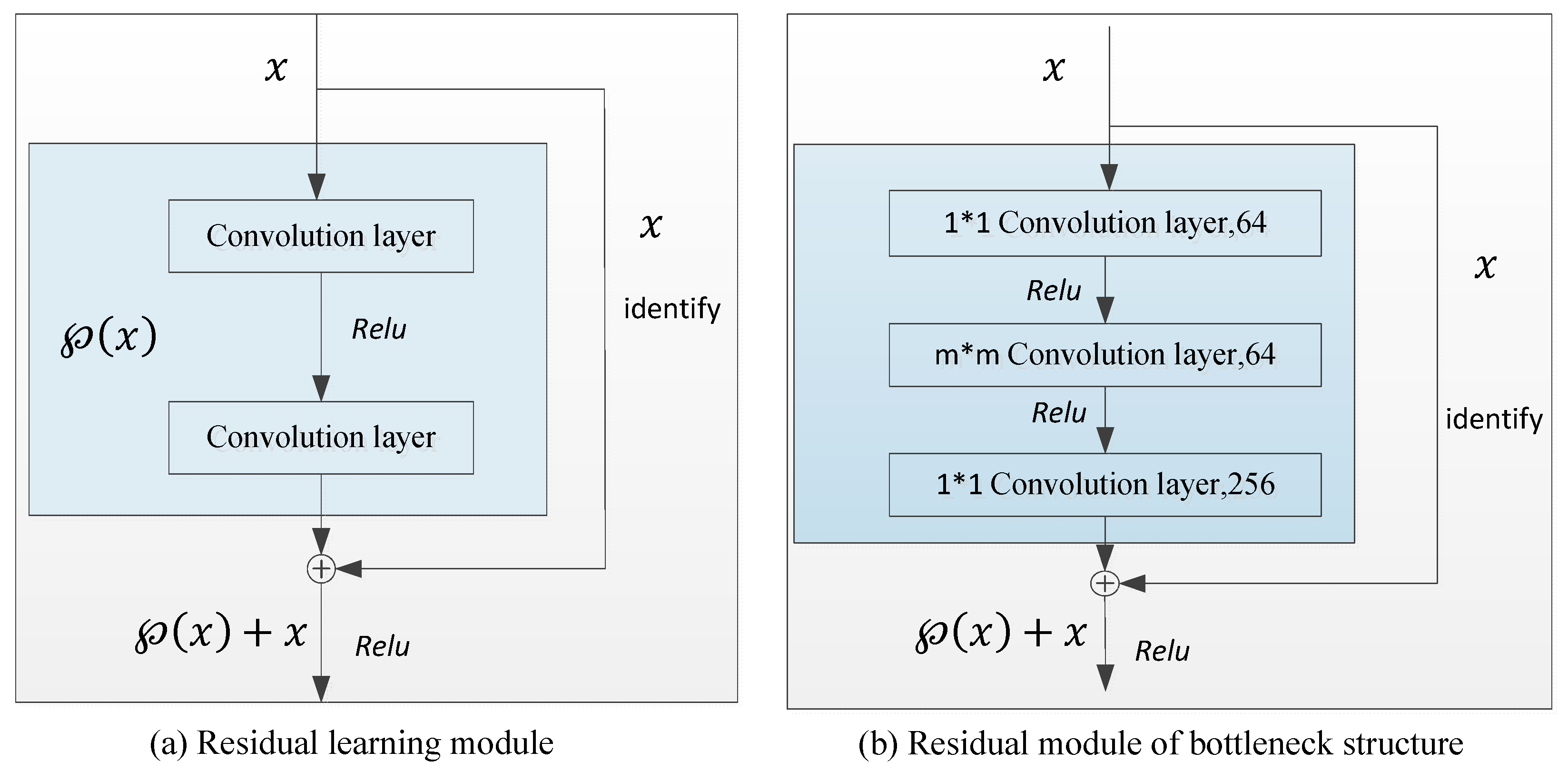
To overcome the above-stated problem, the residual learning approach along with some other approaches was introduced. The ResNet can be defined as $y=\wp \left(\left\{W_i\right\},x\right)+x$, where $\wp \left(\left\{W_i\right\},x\right)$ is the residual mapping function to be learned, $y$ is the output vector of the considered layers, and $x$ is the input vector of the considered layers. As shown in Figure 1a, $\wp =W_{2}Relu\left(W_{1}x\right)$, and $Relu$ is defined as $Relu\left(x\right)=max\left\{0,x\right\}$.

Furthermore, the idea of residual learning is illustrated. We assume that the target mapping $\mathcal{H}\left(x\right)$ is a sub-module of the neural network $\mathsf{\phi }$ that we wish to learn and that $\mathcal{H}\left(x\right)$ may be very complex and difficult to learn. Now, instead of learning $\mathcal{H}\left(x\right)$ directly, the sub-module $\mathsf{\phi }$ learns a residual function $\wp \left(x\right)$ as

$$\wp \left(x\right)=\mathcal{H}\left(x\right)-x.$$

(1)

The original mapping function $\check{x}$ can be expressed as

$$\check{x}=\wp \left(x\right)+x.$$

(2)

That is, $\mathsf{\phi }$ can be composed of two parts: a linear direct mapping $x\to x$ and a nonlinear mapping $\wp \left(x\right)$. If the direct mapping $x\to x$ is optimal, the learning algorithm can easily set the weight parameters of the nonlinear mapping $\wp \left(x\right)$ to 0. If there is no direct mapping, it is very difficult for the nonlinear mapping $\wp \left(x\right)$ to learn the linear mapping $x\to x$. Additionally, He Kaiming’s [26] experiments showed that such a residual structure in the extraction of the image texture and detail features is a significant result.

At present, the ResNet is mainly composed of multiple residual learning modules. However, the consumption in stacking a number of residual learning modules to build a deep neural network is still a little large. Therefore, Zhang et al. [15] presented a residual module structure called a bottleneck, as shown in Figure 1b. Additionally, with the residual learning strategy, a new method named the DnCNN [15] recently showed excellent performance, implicitly removing the latent clean image in the hidden layers. This property motivated us to train a single DnCNN model to tackle several general image denoising tasks, such as Gaussian denoising, single-image super-resolution, and JPEG image deblocking.

In addition, the bottleneck structure module is the key for the ResNet to achieve hundreds or thousands of layers. In Figure 1b, there are three layers in total for the nonlinear part of the bottleneck structure, one $\mathrm{m}\ast \mathrm{m}\left(\mathrm{m}=3\right)$ convolution and two 1∗1 convolutions. Assuming that the dimension of the input data $x$ is 256, the first 1∗1 convolution can reduce the dimensions; at the same time, it also implements cross-channel information fusion to some extent and reduces the input dimension to 64. The second 1∗1 convolution plays a major role in raising the dimension, which causes the output dimension to return back to 256. The input and output dimensions of the middle $\mathrm{m}\ast \mathrm{m}$ convolution fall from the original 256 to 64 by the two 1∗1 convolutions, which greatly reduces the number of parameters and also increases the module depth [23,24]. In order to boost the denoising performance and improve image denoising recognition as much as possible, the bottleneck residual learning module is used to replace the ordinary residual learning module [25].

3. Proposed Aerial-Image Denoising

3.1. The Proposed Method Formulation

At present, all the image denoising methods have a common formulation, as follows:

$$y=x+v,$$

(3)

where $y$ is the observed noisy image generated as the addition of the clean image x and some noise v.

Most of the discriminative denoising models aim to learn a mapping function (Equation (4)) to predict the latent clean image from y:

$$\mathcal{H}\left(y\right)\approx x.$$

(4)

Unlike previous methods, for aerial-image denoising, we follow DnCNN [15] and adopt the residual learning formulation to learn the residual mapping, as follows:

$${\wp }_1\left(y\right)\approx v.$$

(5)

Thus, we have the original function $\check{x}$:

$$\check{x}=y-{\wp }_1\left(y\right).$$

(6)

Formally, to learn the trainable parameters $\lambda$ in the aerial-image denoising model, the averaged mean-square error between the desired image residuals $\left\{{\Delta }_t\right\}$ and estimated residuals $\left\{\wp \right\}$ from noisy input

$$\ell \left(\lambda \right)=\frac{1}{2N}{\displaystyle \sum }_{t=1}^N{\Vert \wp -{\Delta }_t\Vert }_F^2=\frac{1}{2N}{\displaystyle \sum }_{t=1}^N\wp \left(y_t;\lambda \right)-{\left(y_t-x_t\right)}_F^2$$

(7)

can be adopted as the loss function of the residual estimation, where ${\left\{\left(y_t;x_t\right)\right\}}_{t=1}^N$ are $N$ pairs of the noisy–clean training image (patch) and ${\Vert .\Vert }_F^2$ is the Frobenius norm, which, for a matrix $H$, can be calculated by the following formula:

$${\Vert H\Vert }_F^2={{\displaystyle \sum }}_{i,j}{\left|h_{ij}\right|}^2.$$

(8)

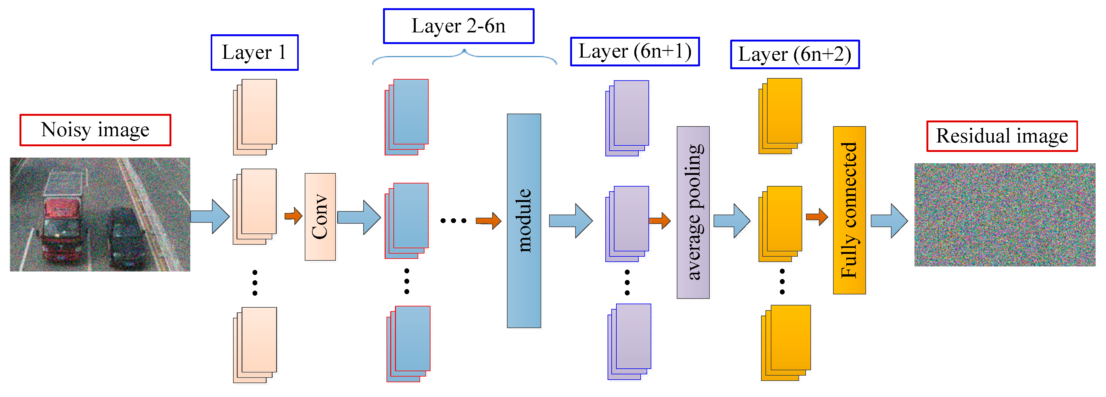
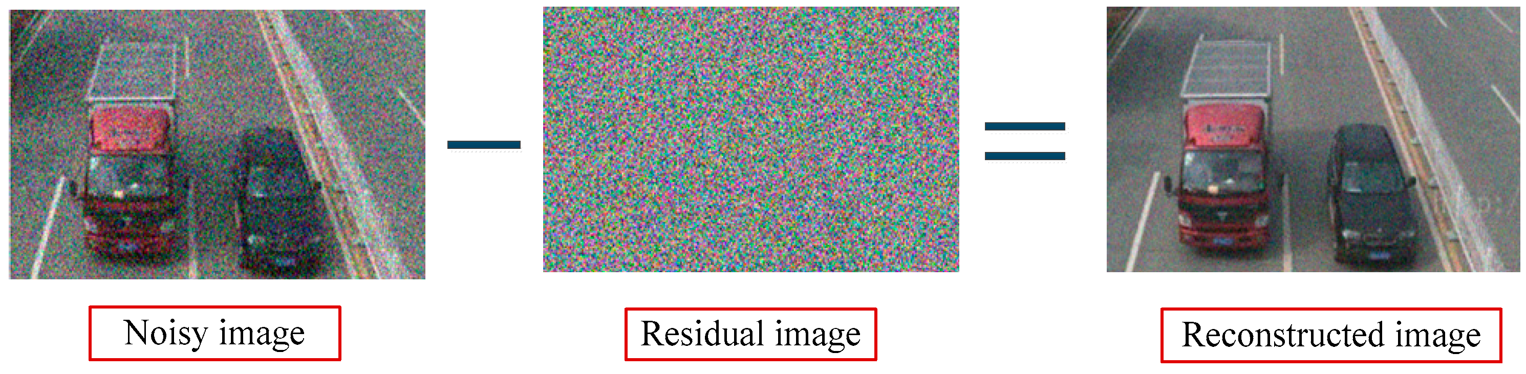
The architecture of the proposed aerial-image denoising model for learning $\wp \left(y\right)$ as shown in Figure 2 and Figure 3 illustrates that the reconstructed denoised image $\check{x}$ is obtained by subtracting the residual image ${\wp }_1\left(y\right)$ from the noisy observation image $y$. In the following, we explain the architecture of the multi-scale learning module for the aerial-image denoising model.

3.2. Multi-Scale Learning Module

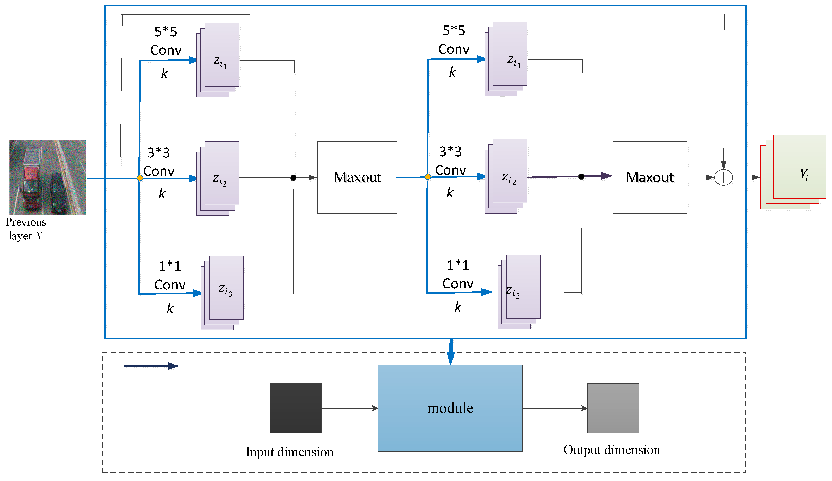
It is assumed that the output of the previous layer $X_{i-1}$ is composed of the $n_{i-1}$ feature mappings ($\mathrm{i}.\mathrm{e}.,n_{i-1}$ channels). Firstly, to produce a set of feature mappings $z_{i_k}$, multi-scale filters are applied to the input data, as follows:

$$z_{i_k}=W_{i_k}\ast \left(X_{i-1}\right)+B_{i_k}$$

(9)

where $W_{i_k}$ and $B_{i_k}$ are the convolutional filters and biases of the $k$th type of the $i$th layer, respectively, and $W_{i_k}$ includes $n_l$ filters of size $n_{i-1}\times f_{i_k}\times f_{i_k}$.

Secondly, each convolution produces $n_l$ feature maps. Therefore, the multi-scale convolution [24] is composed of $K\times n_i$ feature maps. The feature maps are divided into $n_l$ nonoverlapping groups, and the $t$th group is made up of $K$ feature maps, that is, $z_{i_1}^t,z_{i_2}^t,z_{i_3}^t,\cdots ,z_{i_{\mathrm{k}}}^t$; then maximum pooling across $z_{i_1}^t,z_{i_2}^t,z_{i_3}^t,\cdots ,z_{i_k}^t$ is performed by the maxout activation function $\delta (.)$. The function $Y_i^t\left(x,y\right)$,

$$Y_i^t\left(x,y\right)=\delta \left(z_{i_1}^t\left(x,y\right),z_{i_2}^t\left(x,y\right),z_{i_3}^t\left(x,y\right),\cdots ,z_{i_k}^t\left(x,y\right)\right),$$

(10)

is the maxout output of the $t$th group at the position $\left(x,y\right)$, where $z_{i_p}^t\left(x,y\right)\left(p=1,2,\dots ,k\right)$ is the data at a particular position $\left(x,y\right)$ in the $p$th feature map for the $t$th group.

In our paper, the multi-scale convolutional layer comprises three $\left(K=3\right)$ types of filters, $f_{i_1}=5\times 5,f_{i_2}=3\times 3,\mathrm{and}{f}_{i_3}=1\times 1$, as shown in Figure 4. Across the feature maps, the maxout function executes maximum element-wise pooling. During each iteration of the training process, the activation function ensures that the unit with the maximum value in the group is activated. Conversely, the convolution layer feeds the feature map to the maxout activation function.

The difference is that instead of the single 3∗3 convolution kernel in the convolution module, the multiple 1∗1, 3∗3, and 5∗5 convolution kernels are used, so that the convolution layer can observe the input data from different scales, so as to help the different convolution kernels converge to different values, which effectively avoids the collaborative work of the network [27,28].

In Figure 4, $k$ is the scaling parameter, and the three convolutions of unit width are $1\ast 1\ast 16$, $3\ast 3\ast 16$, and $5\ast 5\ast 16$. Then after the transformation of the scaling parameter $k$, the network width is as follows:

$$3\to 3\ast k.$$

(11)

The corresponding three convolution kernels are as follows:

$$\begin{array}{c}1\ast 1\ast 16\to 1\ast 1\ast 16\ast k,\\ 3\ast 3\ast 16\to 3\ast 3\ast 16\ast k,\\ 5\ast 5\ast 16\to 5\ast 5\ast 16\ast k.\end{array}$$

(12)

For the traditional ResNet, when the network depth reaches a certain degree, the effect of the network becomes less obvious [26]. However, the proposed multi-scale ResNet not only increases the network depth, but also makes the network training very easy. The experimental results show the improvement in performance, as detailed in Section 4.2.

3.3. Dropout

Considering the excellence in dropout [6] for CNNs, we incorporated dropout for the image denoising recognition [29,30], where dropout is explained hereunder.

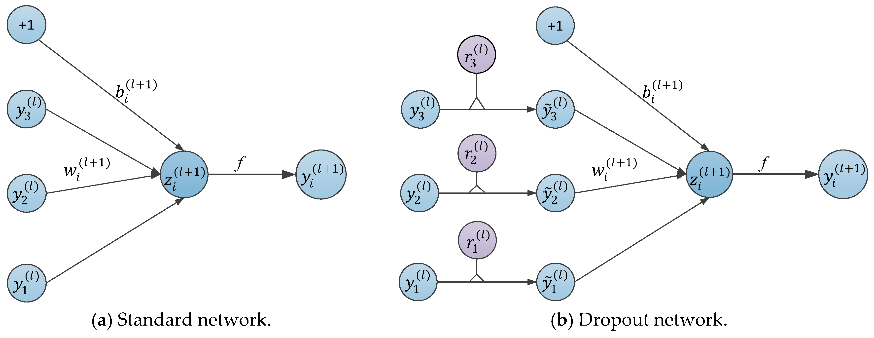
We assume that a neural network with $L$ hidden layers and the feed-forward operation of a standard neural network can be described as follows and can be seen in Figure 5a:

$$z_i^{\left(l+1\right)}=b_i^{\left(l+1\right)}+{\mathit{w}}_i^{\left(l+1\right)}·{\mathit{y}}^l\left(i=1,2,3,\cdots \right)$$

(13)

$$y_i^{\left(l+1\right)}=f\left(z_i^{\left(l+1\right)}\right)\left(i=1,2,3,\cdots \right)$$

(14)

where $l\in \left\{1,2,3,\cdots ,L\right\}$ represents the hidden layers of the network; ${\mathit{y}}^{\left(l\right)}$ represents the vector of outputs from layer $l$ (where ${\mathit{y}}^{\left(0\right)}=\mathit{x}$ is the input); ${\mathit{b}}^{\left(l\right)}$ and $W^{\left(l\right)}$ are the biases and weights of layer $l$, respectively; ${\mathit{z}}^{\left(l\right)}$ represents the vector of inputs into layer $l$; $i$ is any hidden unit; and $f$ is any activation function, such as

$$f\left(x\right)=\frac{1}{1+\exp \left(-x\right)}.$$

(15)

However, with dropout, the feed-forward operation can be expressed as follows and can be seen in Figure 5b:

$$r_j^{\left(l\right)}~\mathrm{Bernoulli}\left(p\right)\left(j=1,2,3,\cdots \right)$$

(16)

$${\tilde{y}}^{\left(l\right)}=r^{\left(l\right)}\ast y^{\left(l\right)}$$

(17)

$$z_i^{\left(l+1\right)}=b_i^{\left(l+1\right)}+w_i^{\left(l+1\right)}·{\tilde{y}}^l\left(i=1,2,3,\cdots \right)$$

(18)

$$y_i^{\left(l+1\right)}=f\left(z_i^{\left(l+1\right)}\right)\left(i=1,2,3,\cdots \right)$$

(19)

where $\mathrm{Bernoulli}()$ is the binomial distribution function and $p$ is the probability that a neuron is discarded, ranging in interval [0, 1], where the probability of being retained is $1-p$; $r^{\left(l\right)}$ is a vector of independent Bernoulli random variables for any layer $l$, and each random variable has a probability $p$ of being 1. To create the thinned outputs ${\tilde{y}}^{\left(l\right)}$, the vector is sampled and multiplied with the output elements of the layer, $y^{\left(l\right)}$. Then the process in which ${\tilde{y}}^{\left(l\right)}$ is used as input to the next layer begins to be applied for each layer.

In the multi-scale learning module, when the input and output neurons remain unchanged, half of the hidden neurons in the network are deleted randomly (temporary), so that the corresponding parameters will not be updated when the network is propagating in reverse. At the time of training, the dropout is equivalent to training a subnet of the whole network every time. If there are $n$ nodes in the network, the number of available subnets should be $2^n$. When $n$ is large enough, the subnets used in each training will not be the same. Finally, the whole network can be regarded as the average of the multiple subnet models. By doing this, the training set can avoid overfitting of a certain subnet and enhance the generalization ability of the network.

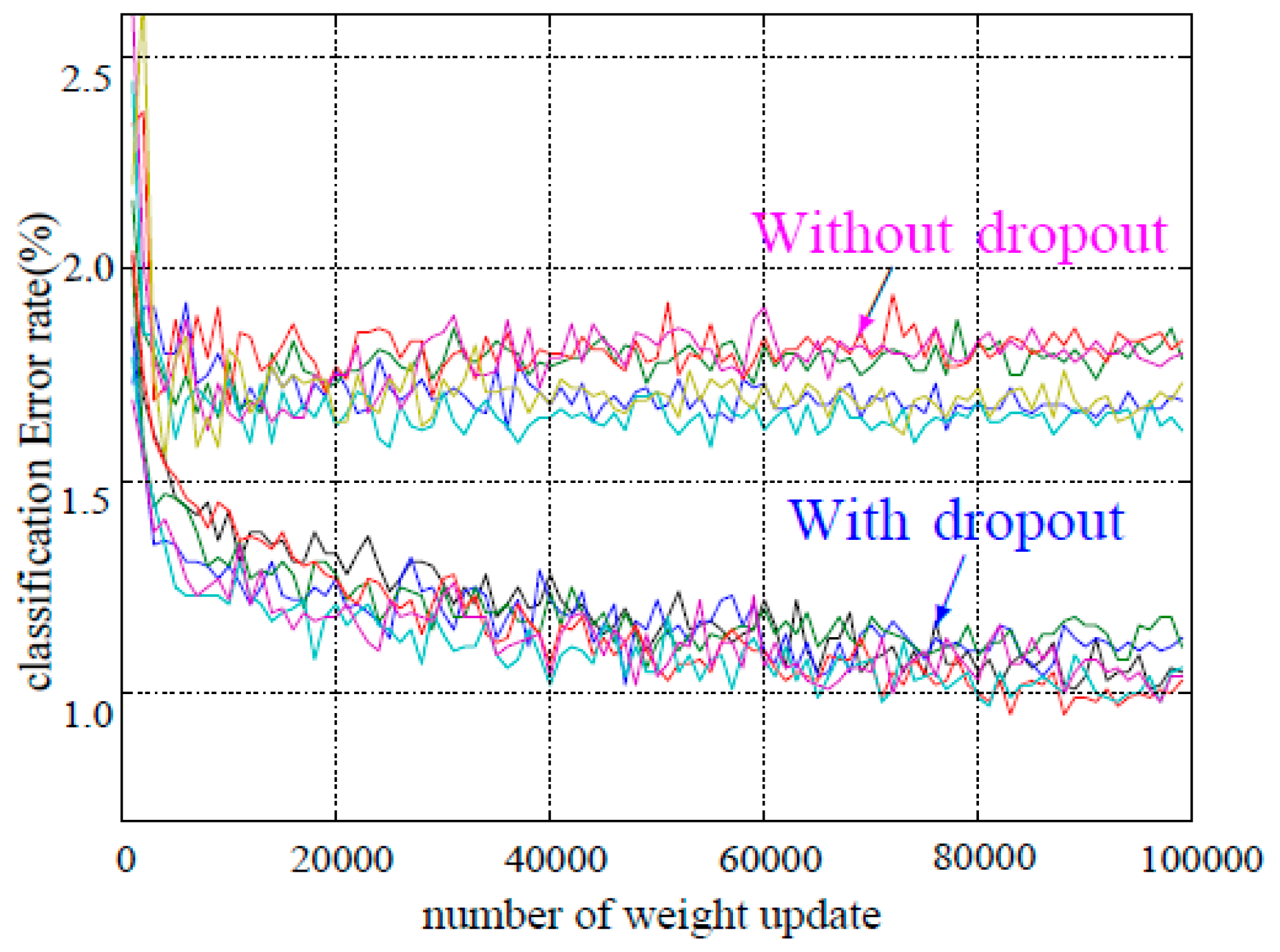
As described above, dropout helps the network retain robustness. Figure 6 shows the test error rates obtained for many different datasets (CIFAR-10, MNIST, etc.) as training progressed. As seen from two separate clusters of trajectories, the same datasets trained with and without dropout had significantly different test errors, and dropout brought a great improvement across all architectures. For our aerial-image denoising model, we found that incorporating dropout boosted the accuracy of the model and made the training process faster. The experimental results show that the dropout location and drop ratio $p$ affected the network performance, as detailed in Section 4.2.2.

4. Experimental Results and Setting

The main purpose of the experimental work of this paper was to confirm the performance of our proposed approach in the aerial-image denoising recognition model.

4.1. System Environment

The computer configuration used in the experimental environment was as shown in

Table 1. The machine configuration used in experimental environment.

Computer Configuration
Processor	Intel(R) Core(TM) i7-7700HQ CPU @ 2.90 GHz
GPU	NVIDIA GeForce GTX1050 Ti
RAM	8 GB
Hard disk	SSD 256 GB
Operating system	Windows 7 @ 64 bit
Test framework	Tensorflow

.

In our experiment, the model for Gaussian denoising was trained with noise levels $\mathsf{\sigma }=10$ $\mathsf{\sigma }=15$, and $\mathsf{\sigma }=25$ independently. Firstly, we considered the images of the Caltech [31] database to train the model. The database is a publicly available aerial database that comprises an aircraft dataset and a vehicle dataset. We mixed 475 images from the vehicle dataset and 350 images from the aircraft dataset to train the model. Finally, 55 images were randomly selected from the two datasets, which were not included in the training period but were used for the test model.

4.2. Parameter Setting Analysis

4.2.1. Experimental Parameters

In the experiment, the momentum random gradient descent method was used. At the 50th and 100th epochs, the learning rate increased by a factor of 0.1, and the total number of epoch runs was 150.The experiment ran on two blocks of NVIDIA GeForce GTX1050 Ti, and mini-batch had 100 samples for each GPU. In addition, other parameters are shown in

Table 2. The parameter in experimental environment.

Parameter
Loss Function	Initial Learning Rate	Drop Probability	Momentum	Weight Decay
Cross-entropy	0.1	0.3	0.9	0.0005

.

4.2.2. Selecting Dropout Location

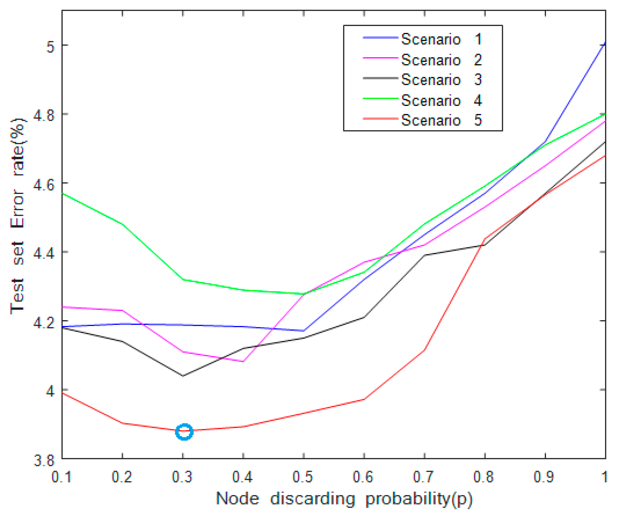
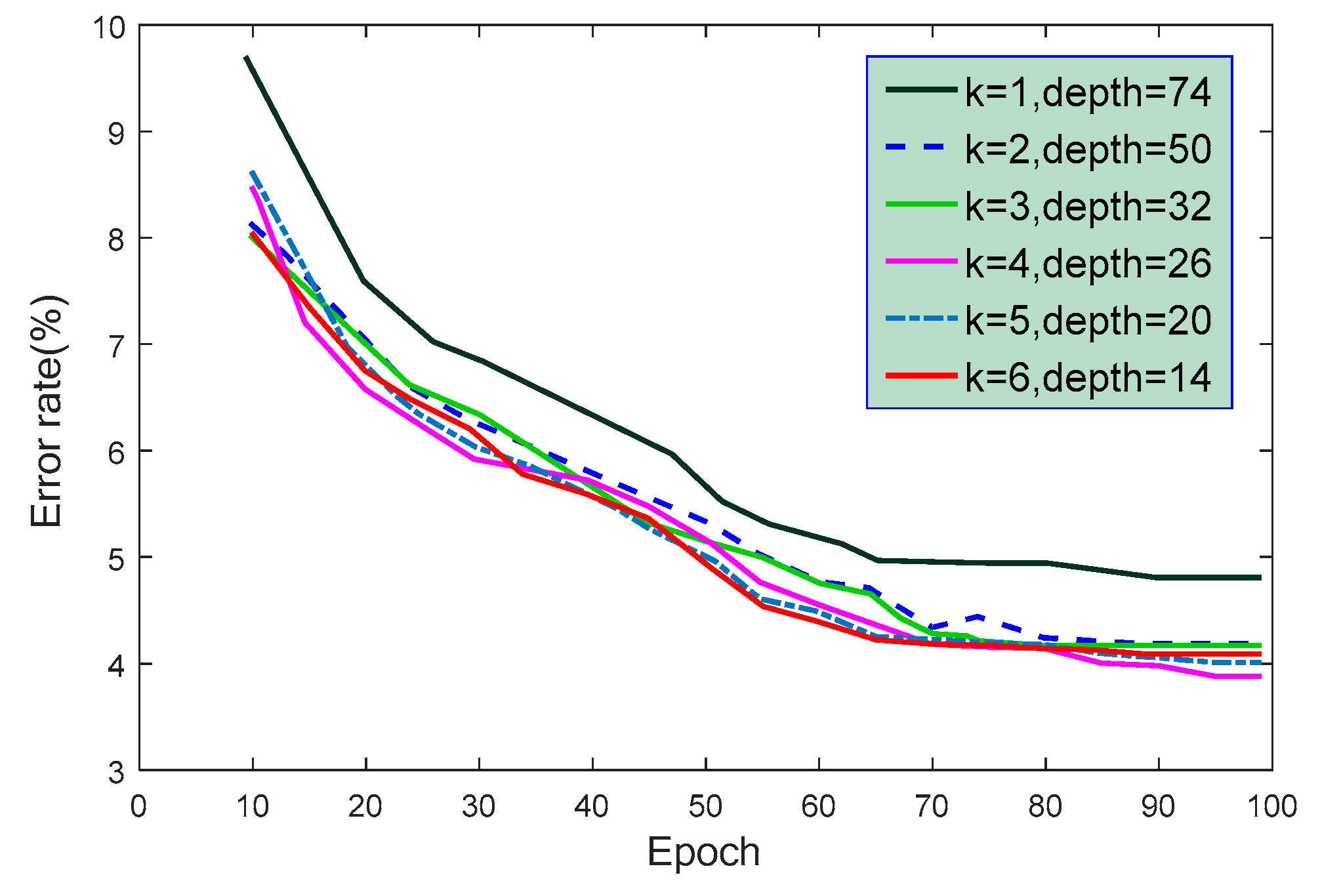
From Section 3.3, we know that dropout can effectively avoid network overfitting and improve the denoising performance. Therefore, it is necessary to discuss the influence of dropout location on the network performance. Figure 7 and Figure 8 show the different dropout locations in the multi-scale residual learning module and the influence of parameter $p$ (drop ratio) on the network image denoising recognition performance, respectively.

From Figure 8, we can see that in Scenario 5, when $p$ was 0.3, the error rate of the test set was the smallest, 3.88%. On the contrary, in Scenario 4, when $p$ was 0.3, the error rate of the test set was the largest, 4.32%. Therefore, for the proposed multi-scale ResNet, we adopted Scenario 5, that the node discarding probability $p$ is 0.3 and a dropout layer is added before the full connection layer.

4.2.3. Network Depth

Instead of the network depth being based on the experience, the optimal network depth was acquired through the experiments. The multi-scale ResNet structure includes $3n$ multi-scale residual learning modules with two layers of convolution for each learning module, and the entire network has $\left(6n+2\right)$ layers. In addition, there is a scaling parameter $k$ for each convolution layer. Each layer consists of three different scale convolutions 1∗1, 3∗3, and 5∗5, and the network width is $3\ast k$. In order to explore the effect of different scaling parameters and depths on the network performance, we conducted some experiments on the Caltech dataset. The results are shown in Figure 9 and

Table 3. The error rate of test set under different network structures, where $k$ is the scaling parameter and $n$ is the number of learning modules.

Model States
Model Number	$\mathit{k}$	$\mathit{n}$	Network Depth	Parameters	Error Rate
i	1	12	74	12.9 M	4.813%
ii	1	16	98	18.7 M	4.913%
iii	1	20	122	22.8 M	4.965%
iv	2	8	50	36.1 M	4.191%
v	3	5	32	47.8 M	4.178%
vi	3	6	38	59.1M	4.238%
vii	4	4	26	66.4 M	3.883%
viii	5	3	20	76.4 M	4.012%
ix	6	2	14	81.3 M	4.099%

.

It can be seen from Table 3 that with the increase in the parameter $k$, the network depth decreased. However, the model became more and more complex, and more and more parameters needed to be trained. Accordingly, the recognition error rate of the model for the test set also became continually lower. In Table 3, the scaling parameter of model 8 was 5, which was larger than that of model 7, and the number of parameters was also more than 10 M, but the accuracy rate declined. The main reasons may be that the structure of model 8 was too complex and the number of parameters was too great, which increased the training difficulty, and a slight overfitting phenomenon occurred. In addition, we can see from Figure 3 that with the increase in training times, the error rate tended to be stable. Therefore, in the experiment, in order to obtain the best network effect, the scaling parameter was set to 4 and the network depth was set to about 26.

To further evaluate the performance of the proposed model, it was necessary to test the running state of the model under conditions of different scaling parameters and network depths, as shown in

Table 4. The running state of model under different scaling parameters and network depths, where “—” indicates that GPU resources were exhausted and could not be trained (blue font indicates the best).

Model State
$\mathit{k}$	$\mathit{n}$	Network Depth	Parameters (M)	Training Situation	Error Rate (%)
1	20	122	22.8	Normal training	4.965
1	21	128	25.3	—
1	22	134	26.8	—
2	8	50	36.1	Normal training	4.229
2	9	56	40.9	—
2	10	62	43.9	—
3	6	38	59.1	Normal training	4.232
3	7	44	68.0	—
3	8	50	69.5	—
4	4	26	66.4	Normal training	3.883
4	5	32	83.6	—
4	6	38	88.5	—
5	3	20	76.4	Normal training	4.012
5	4	26	105.5	—
5	5	32	108.3	—
6	2	14	81.3	Normal training	4.099
6	3	20	110.2	—
6	4	26	114.7	—

.

As we can see from Table 4, with the increase in the scaling parameter $k$, the number of parameters of the network training also increased. When the scaling parameter was 4, the network could only be added to 26 layers, and the training parameter is 66.4 M. When the number of layers was increased, the GPU resources were exhausted. In addition, when the scaling parameter increased to 5, 76.4 M parameters could be trained at most. In addition, when the number of parameters reached about 70 M, the proposed multi-scale ResNet algorithm did not have serious overfitting problems.

It also can be seen from Table 4 that the proposed multi-scale ResNet (scaling parameter of 4 and network depth of 26) was the best. The error rate on the Caltech dataset was about 3.883%. To further study the impact of the network depth on the network performance, we fixed the scaling parameters to 4, slightly adjusting the number of groups of learning modules.

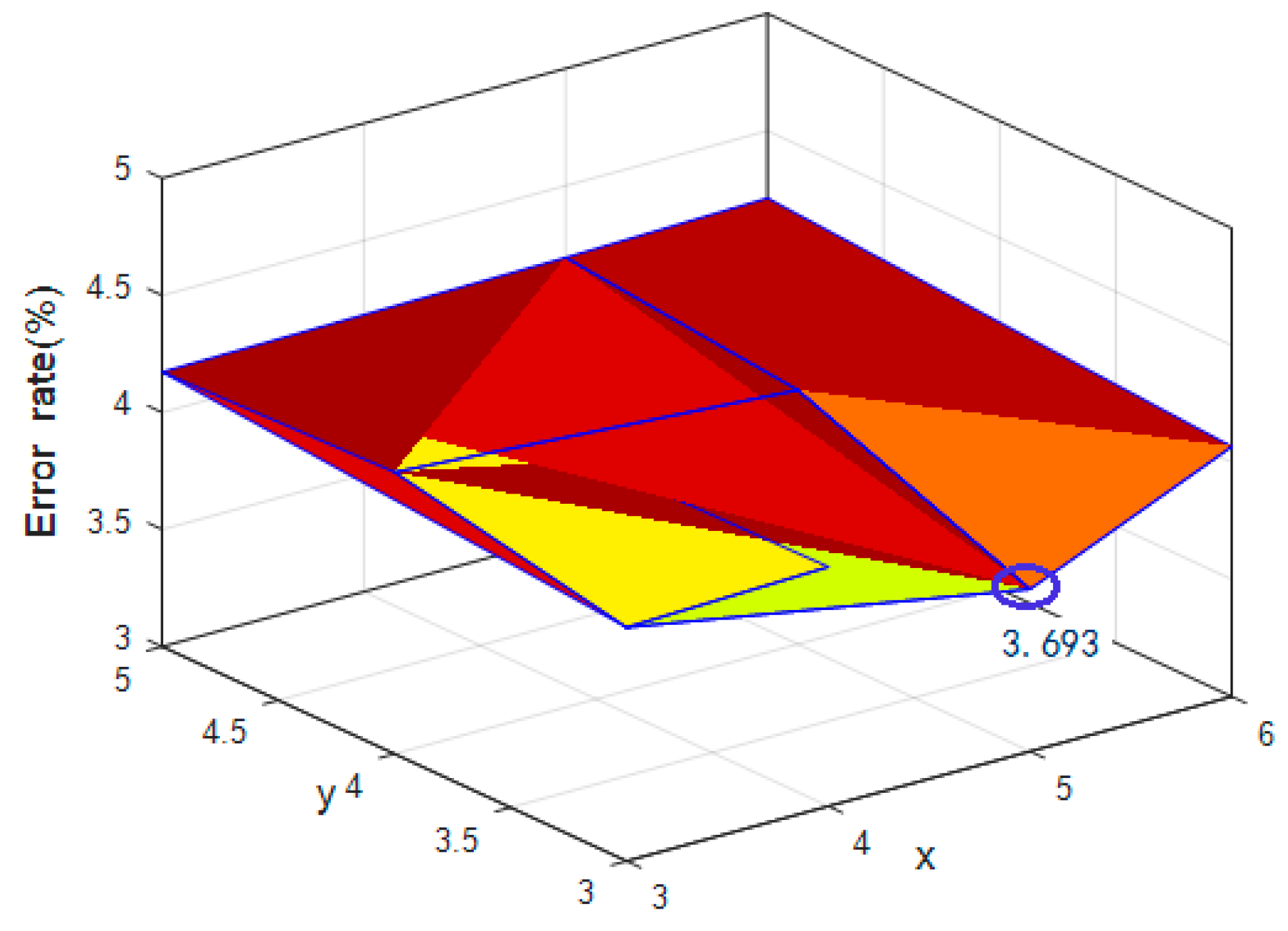
The multi-scale ResNet consists of three groups of learning modules, and each group contains $n$ learning modules. To obtain the ideal number groups of learning modules, we changed the numbers of learning modules in each group so that they were not completely equal. Supposing that the numbers of learning modules in the groups are x, y, and z ($x$ being the number of modules close to the input layer, $y$ being the number of modules close to the output layer, and $z$ being the fixed scaling parameter), the value of $z$ was 4, and the values of $x$ and $y$ were changed. The experimental results are shown in Figure 10.

As can be seen from Figure 10, when $x$ = 5, $y$ = 3, and $z$ = 4, the error rate was 3.693%, which was much better than for all variables being equal to 4. This indicates that appropriately increasing the number of modules that are close to the input layer can better capture the original features of the picture and help to improve the network performance. In the next part, we describe the use of these parameters to evaluate our proposed aerial-image denoising recognition methods.

4.2.4. Model Architecture

In this study, as we have shown in the model architecture in Figure 2, the model was trained by the minimizing the cost function in Equation (11), and the model architecture had a depth of (6n + 2) layers. The image size of 32∗32∗3 was inputted and passed through the 3∗3 convolution kernel with 16 convolution kernels, and the output of the model was 32∗32∗16; then these data were passed through the 6n convolution layers and average pool layer, followed by a dropout operation, and were finally passed through a full connection layer and subjected to a softmax operation. In this model, residual learning was adopted to learn the mapping $\wp \left(y\right),$ and batch normalization was incorporated to increase the model’s accuracy and speed up the training performance. It was seen that the proposed multi-scale ResNet for a small training dataset has promising advantages for training deep networks and further improves the network accuracy.

4.3. Comparison with State-of-the-Art Algorithms

In this section, we use the optimal parameters that were obtained in Section 4.2 to evaluate the recognition ability of the proposed improved multi-scale residual neural network learning approach. We compared our results with other aerial-image denoising methods from the existing literature, such as PNN [32], BM3D [33], SRCNN [34], WNNM [35], and DnCNN [15], where x = 5, y = 3, and z = 4. The experimental results revealed that our model benefits from multi-scale residual learning, parameter setting, and particular image sizes, as can be seen in

Table 5. The average results of our aerial-image model, where the multi-scale residual learning network (ResNet) was the proposed aerial-image denoising method in the paper. The corresponding experimental parameters were $x$ = 5, $y$ = 3, scaling parameter $z$ = 4, and network depth of 26 (blue font indicates the best).

Noise Level ($\mathsf{\sigma }$)	Methods	Image Size of 64 × 64, with Dropout
PSNR/SSIM	PNN	Multi-Scale ResNet	SRCNN	BM3D	WNNM	DnCNN
$\mathsf{\sigma }$ = 10	38.485/0.9000	39.482/0.9271	38.551/0.9211	38.494/0.9004	38.494/0.9001	39.466/0.9271
$\mathsf{\sigma }$ = 15	36.388/0.8881	38.607/0.9202	37.112/0.9000	36.993/0.9001	36.379/0.8746	38.007/0.9202
$\mathsf{\sigma }$ = 25	35.553/0.7003	36.998/0.9193	36.996/0.9303	36.261/0.9184	36.118/0.7839	36.767/0.9192

. Figure 11, Figure 12, Figure 13, Figure 14, Figure 15 and Figure 16 show the randomly selected images reconstructed by the model trained with the training sample.

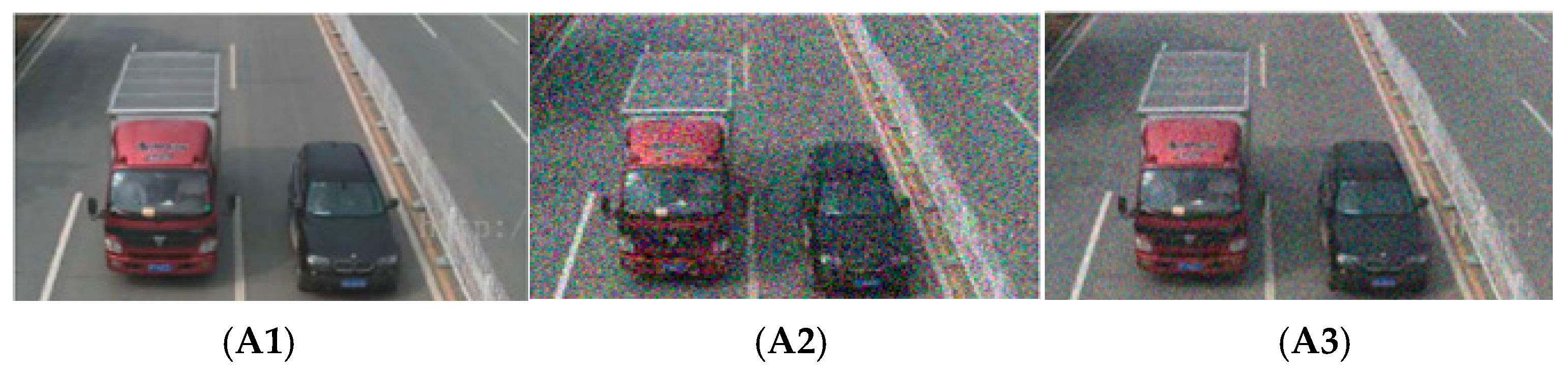
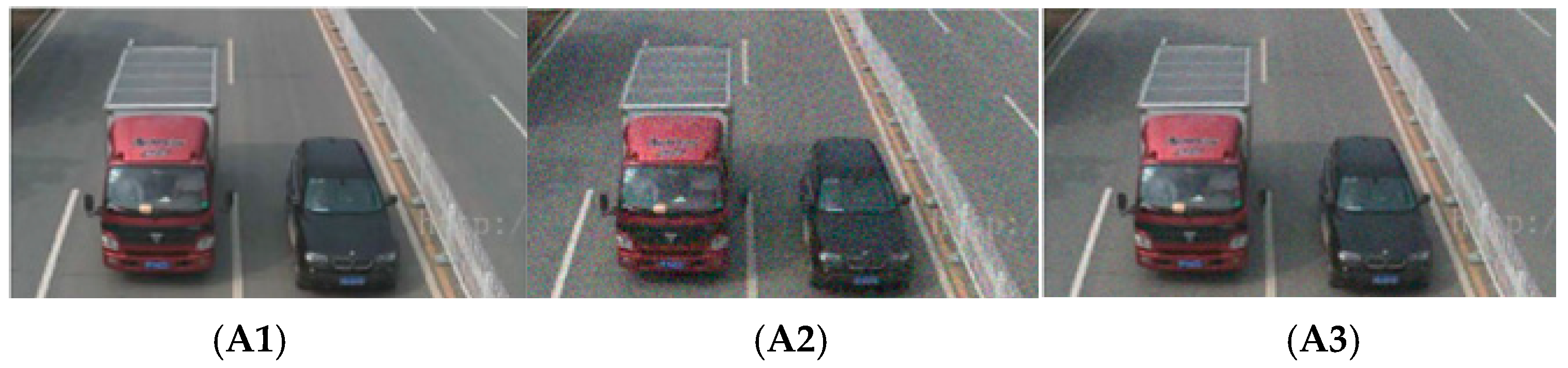
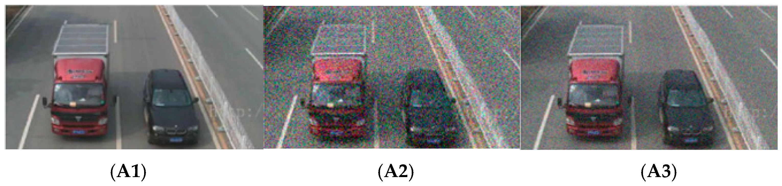
Figure 11, Figure 12, Figure 13, Figure 14, Figure 15 and Figure 16 with different noise parameters are used for comparison to illustrate our experimental results. We randomly selected some images from the test model, as shown in Figure 11, Figure 12 and Figure 13, which show the evaluation of the proposed model trained on 825 images, each with an image size of 64 × 64. From the three figures, we can see that the reconstructed images were similar to the original images; Figure 11 shows the effect better, as the reconstructed image was more similar to the original image because of low noise ($\mathsf{\sigma }=10$). A similar conclusion can be observed by comparing Figure 14, Figure 15 and Figure 16 (Figure 14 is the most apparent).

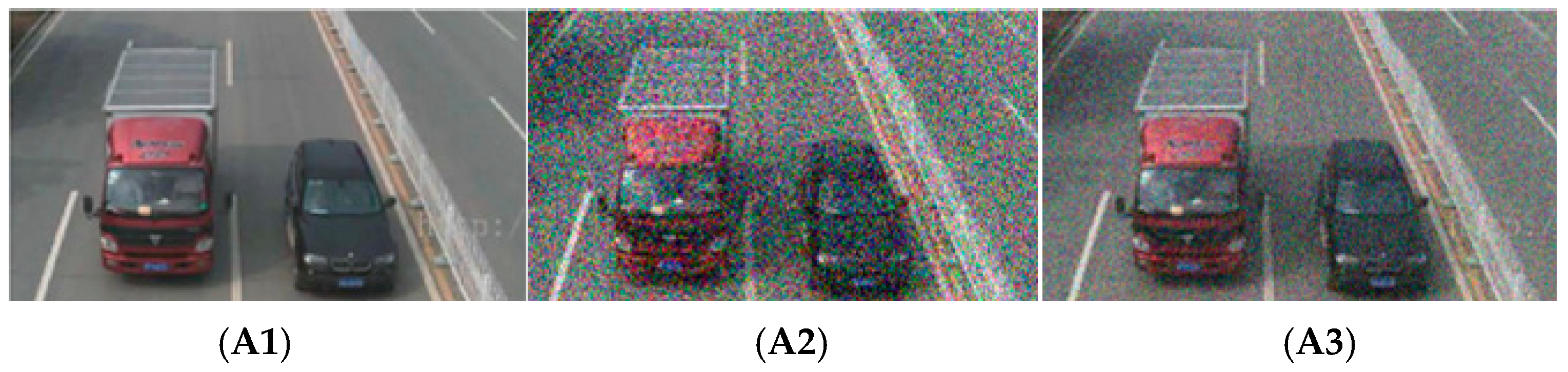
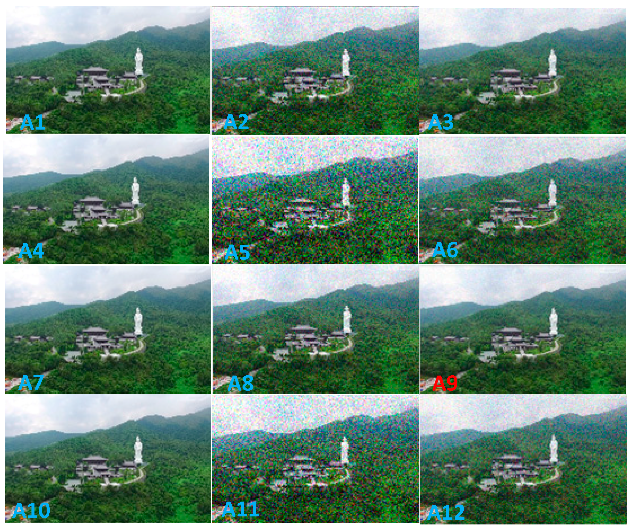
Figure 14, Figure 15 and Figure 16 also represent the evaluation of the proposed model trained on 825 images, each with an image size of 180 × 180. Compared with Figure 11, the reconstructed images of Figure 14 are more similar to the original image, which implies the proposed model benefited from a particular image size. Furthermore, comparing Figure 12 and Figure 15 and Figure 13 and Figure 16 separately, a similar conclusion can be observed. The same conclusion is also reached from Figure 17.

We compared our model performance with images of the same image size. Table 5 shows the average results of the proposed model trained on an image size of 64 × 64, the training sample size of 825 images, and with dropout; it can be seen that the proposed model improved the reconstructed image quality by about 0.167/0.001 over the DnCNN and by about 0.931/0.006 over the SRCNN at $\mathsf{\sigma }$ = 10 and was better than the other methods in terms of PSNR/SSIM values at $\mathsf{\sigma }=10$, $\mathsf{\sigma }=15$, and $\mathsf{\sigma }=25$.

Similarly,

Table 6. The average results of our aerial-image model, where the multi-scale residual learning network (ResNet) was the proposed aerial-image denoising method in the paper. The corresponding experimental parameters were $x$ = 5, $y$ = 3, scaling parameter $z$ = 4, and network depth of 26 (blue font indicates the best).

Noise Level ($\mathsf{\sigma }$)	Methods	Image Size of 180 × 180, with Dropout
PSNR/SSIM	PNN	Multi-Scale ResNet	SRCNN	BM3D	WNNM	DnCNN
$\mathsf{\sigma }$= 10	40.114/0.9009	40.987/0.9652	40.478/0.9622	40.115/0.9195	40.114/0.9191	40.582/0.9642
$\mathsf{\sigma }$ = 15	38.572/0.9441	40.208/0.9597	39.442/0.9501	39.028/0.9447	39.005/0.9448	39.881/0.9597
$\mathsf{\sigma }$ = 25	37.316/0.9311	38.448/0.9421	37.411/0.9400	37.401/0.9338	37.189/0.9278	37.644/0.9420

exhibits the model performance with an image size of 180 × 180, the training sample size of 825 images, and with dropout. Again, it can be seen that the proposed model improved the average reconstructed image quality at $\mathsf{\sigma }=10$, $\mathsf{\sigma }=15,$ and $\mathsf{\sigma }=25$. However, in comparison with the results in Table 5 and Table 6, we found this image size affected the model performance; the performance of the model trained on the image size of 180 × 180 with dropout was better than that with the image size of 64 × 64 with dropout. This conclusion is consistent with the above (Figure 11, Figure 12, Figure 13, Figure 14, Figure 15 and Figure 16). Furthermore, comparing Table 6 and

Table 7. The average results of our aerial-image model, where the multi-scale residual learning network (ResNet) was the proposed aerial-image denoising method in the paper. The corresponding experimental parameters were $x$ = 5, $y$ = 3, scaling parameter $z$ = 4, and network depth of 26 (blue font indicates the best).

Noise Level ($\mathsf{\sigma }$)	Methods	Image Size of 180 × 180, without Dropout
PSNR/SSIM	PNN	Multi-Scale ResNet	SRCNN	BM3D	WNNM	DnCNN
$\mathsf{\sigma }$ = 10	37.660/0.8796	39.481/0.9424	38.003/0.9008	38.104/0.9103	37.661/0.9001	38.117/0.9424
$\mathsf{\sigma }$ = 15	36.782/0.8982	38.115/0.9331	37.180/0.9115	37.178/0.9112	36.703/0.8954	37.380/0.9321
$\mathsf{\sigma }$ = 25	35.116/0.8716	36.662/0.9004	35.333/0.8894	35.371/0.8990	35.003/0.8541	35.773/0.9010

, we also found that the incorporation of dropout for image recognition (dropout location is critical) significantly improved the model network performance. This conclusion is consistent with Section 4.2.2.

5. Summary and Conclusions

In this paper, we propose an efficient deep CNN model for the denoising of aerial images with a small training dataset. Unlike most of the aerial-image denoising methods, which approximate a latent clean image from an observed noisy image, the proposed model approximates the noise from the observed noisy image. By combining multi-scale residual learning and dropout, regarding the influence of the network depth and the number of learning modules in each group on the network performance, we not only speed up the training process, but also improve the denoising performance of the model. More importantly, although the deep architecture has a better performance with a large training dataset, the proposed aerial-image denoising model was trained with small dataset and achieved competitive results. With a small training dataset, the experimental results showed that the proposed aerial-image denoising model has better performance than the existing image denoising methods. In the future, the performance expectation of the model will be improved by stacking more multi-scale competitive modules.

References

- Naylor, B.J.; Endress, B.A.; Parks, C.G. Multiscale Detection of Sulfur Cinquefoil Using Aerial Photography. Rangel. Ecol. Manag. 2005, 58, 447–451. [Google Scholar] [CrossRef]
- Chang, S.G.; Yu, B.; Vetterli, M. Adaptive wavelet thresholding for image denoising and compression. IEEE Trans. Image Process. 2000, 9, 1532–1546. [Google Scholar] [CrossRef] [PubMed] [Green Version]
- Dong, W.; Zhang, L.; Shi, G.; Li, X. Nonlocally Centralized Sparse Representation for Image Restoration. IEEE Trans. Image Process. 2013, 22, 1618–1628. [Google Scholar] [CrossRef] [PubMed]
- Hou, Y.; Zhao, C.; Yang, D.; Cheng, Y. Comments on “Image Denoising by Sparse 3-D Transform-Domain Collaborative Filtering”. IEEE Trans. Image Process. 2011, 1, 268. [Google Scholar]
- Elad, M.; Aharon, M. Image Denoising Via Learned Dictionaries and Sparse representation. In Proceedings of the 2006 IEEE Computer Society Conference on Computer Vision and Pattern Recognition, New York, NY, USA, 17–22 June 2006; pp. 895–900. [Google Scholar]
- Hinton, G.E.; Srivastava, N.; Krizhevsky, A.; Sutskever, I.; Salakhutdinov, R.R. Improving neural networks by preventing co-adaptation of feature detectors. Comput. Sci. 2012, 3, 212–223. [Google Scholar]
- Schmidhuber, J. Deep learning in neural networks: An overview. Neural Netw. 2015, 61, 85–117. [Google Scholar] [CrossRef] [PubMed] [Green Version]
- Tan, Z.; Wei, H.; Chen, Y.; Du, M.; Ye, S. Design for medical imaging services platform based on cloud computing. Int. J. Big Data Intell. 2016, 3, 270. [Google Scholar] [CrossRef]
- Yu, S.; Cheng, Y.; Su, S.; Cai, G.; Li, S. Stratified pooling based deep convolutional neural networks for human action recognition. Multimedia Tools Appl. 2017, 76, 13367–13382. [Google Scholar] [CrossRef]
- Frost, V.; Stiles, J.; Shanmugan, K.; Holtzman, J. A model for radar images and its application to adaptive digital filtering of multiplicative noise. IEEE Trans. Pattern Anal. Mach. Intell. 1982, 2, 157–166. [Google Scholar] [CrossRef]
- Kuan, D.; Sawchuk, A.; Strand, T.; Chavel, P. Adaptive noise smoothing filter for images with signal-dependent noise. IEEE Trans. Pattern Anal. Mach. Intell. 1985, 2, 165–177. [Google Scholar] [CrossRef]
- Zhang, Q.; Yuan, Q.; Li, J.; Yang, Z.; Ma, X. Learning a dilated residual network for SAR image despeckling. Remote Sens. 2017, 10, 196. [Google Scholar] [CrossRef]
- Wei, Y.; Yuan, Q.; Shen, H.; Zhang, L. Boosting the accuracy of multispectral image pansharpening by learning a deep residual network. IEEE Geosci. Remote Sens. Lett. 2017, 14, 1795–1799. [Google Scholar] [CrossRef]
- Yuan, Q.; Wei, Y.; Meng, X.; Shen, H.; Zhang, L. A multiscale and multidepth convolutional neural network for remote sensing imagery pan-sharpening. IEEE J. Sel. Top. Appl. Earth Obs. Remote Sens. 2018, 11, 978–989. [Google Scholar] [CrossRef]
- Zhang, K.; Zuo, W.; Chen, Y.; Meng, D.; Zhang, L. Beyond a Gaussian Denoiser: Residual Learning of Deep CNN for Image Denoising. IEEE Trans. Image Process. 2017, 26, 3142–3155. [Google Scholar] [CrossRef] [PubMed] [Green Version]
- Oliveira, T.P.; Barbar, J.S.; Soares, A.S. Computer network traffic prediction: A comparison between traditional and deep learning neural networks. Int. J. Big Data Intell. 2016, 3, 28–37. [Google Scholar] [CrossRef]
- Krizhevsky, A.; Sutskever, I.; Hinton, G.E. Imagenet classification with deep convolutional neural networks. In Proceedings of the 25th International Conference on Neural Information Processing Systems, Lake Tahoe, NV, USA, 3–8 December 2012; Curran Associates Inc.: Red Hook, NY, USA, 2012; Volume 1, pp. 1097–1105. [Google Scholar]
- Greenspan, H.; Ginneken, B.V.; Summers, R.M. Guest editorial deep learning in medical imaging: Overview and future promise of an exciting new technique. IEEE Trans. Med. Imaging 2016, 35, 1153–1159. [Google Scholar] [CrossRef]
- Gebraeel, N.Z.; Lawley, M.A. A neural network degradation model for computing and updating residual life distributions. IEEE Trans. Autom. Sci. Eng. 2008, 5, 154–163. [Google Scholar] [CrossRef]
- Sun, J.; Cao, W.; Xu, Z.; Ponce, J. Learning a convolutional neural network for non-uniform motion blur removal. In Proceedings of the 2015 IEEE Conference on Computer Vision and Pattern Recognition (CVPR), Boston, MA, USA, 7–12 June 2015; pp. 769–777. [Google Scholar]
- Dhungel, N.; Carneiro, G.; Bradley, A.P. A deep learning approach for the analysis of masses in mammograms with minimal user intervention. Med. Image Anal. 2017, 37, 114–128. [Google Scholar] [CrossRef] [PubMed] [Green Version]
- Bruna, J.; Sprechmann, P.; LeCun, Y. Super-resolution with deep convolutional sufficient statistics. arXiv 2015, arXiv:1511.05666. [Google Scholar]
- Qin, P.; Cheng, Z.; Cui, Y.; Zhang, J.; Miao, Q. Research on Image Colorization Algorithm Based on Residual Neural Network. In CCF Chinese Conference on Computer Vision; Springer: Singapore, 2017; pp. 608–621. [Google Scholar]
- Szegedy, C.; Liu, W.; Jia, Y.; Sermanet, P.; Reed, S.; Anguelov, D.; Erhan, D.; Vanhoucke, V.; Rabinovich, A. Going deeper with convolutions. In Proceedings of the 2015 IEEE Conference on Computer Vision and Pattern Recognition (CVPR), Boston, MA, USA, 7–12 June 2015; pp. 1–9. [Google Scholar]
- Murad, A.; Pyun, J.-Y. Deep Recurrent Neural Networks for Human Activity Recognition. Sensors 2017, 17, 2556. [Google Scholar] [CrossRef] [PubMed]
- He, K.; Zhang, X.; Ren, S.; Sun, J. Identity Mappings in Deep Residual Networks. In Proceedings of the 14th European Conference on Computer Vision, Amsterdam, The Netherlands, 11–14 October 2016; pp. 630–645. [Google Scholar]
- Rajkomar, A.; Lingam, S.; Taylor, A.G.; Blum, M.; Mongan, J. High-throughput classification of radiographs using deep convolutional neural networks. J. Digit. Imaging 2017, 30, 95–101. [Google Scholar] [CrossRef] [PubMed]
- Ioffe, S.; Szegedy, C. Batch Normalization: Accelerating Deep Network Training by Reducing Internal Covariate Shift. arXiv 2015, arXiv:1502.03167. [Google Scholar]
- Dahl, G.E.; Sainath, T.N.; Hinton, G.E. Improving deep neural networks for LVCSR using rectified linear units and dropout. In Proceedings of the 2013 IEEE International Conference on Acoustics, Speech and Signal Processing, Vancouver, BC, Canada, 26–31 May 2013; Volume 26, pp. 8609–8613. [Google Scholar]
- Srivastava, N.; Hinton, G.; Krizhevsky, A.; Sutskever, I.; Salakhutdinov, R. Dropout: A simple way to prevent neural networks from overfitting. J. Mach. Learn. Res. 2014, 15, 1929–1958. [Google Scholar]
- Clevert, D.A.; Unterthiner, T.; Hochreiter, S. Fast and accurate deep network learning by exponential linear units (ELUs). arXiv 2015, arXiv:1511.07289. [Google Scholar]
- Masi, G.; Cozzolino, D.; Verdoliva, L.; Scarpa, G. Pansharpening by convolutional neural networks. Remote Sens. 2016, 8, 594. [Google Scholar] [CrossRef]
- Dabov, K.; Foi, A.; Katkovnik, V.; Egiazarian, K. Image denoising by sparse 3-D transform-domain collaborative filtering. IEEE Trans. Image Process. 2007, 16, 2080–2095. [Google Scholar] [CrossRef] [PubMed]
- Dong, C.; Loy, C.C.; He, K.; Tang, X. Image super-resolution using deep convolutional networks. IEEE Trans. Pattern Anal. Mach. Intell. 2016, 38, 295–307. [Google Scholar] [CrossRef] [PubMed]
- Schmidt, U.; Roth, S. Shrinkage fields for effective image restoration. In Proceedings of the 2014 IEEE Conference on Computer Vision and Pattern Recognition, Columbus, OH, USA, 23–28 June 2014; pp. 2774–2781. [Google Scholar]
Figure 1.
Residual learning network.
Figure 2.
The architecture of the model for aerial-image denoising; is the number of learning modules (the size of is discussed in Section 4.2.3), and the module is a multi-scale residual learning module (see Figure 4).
Figure 3.
Reconstruction phase of the proposed model.
Figure 4.
Multi-scale residual learning module.
Figure 5.
A comparison of the basic operations between the standard and dropout networks.
Figure 6.
Test error for different datasets with and without dropout.
Figure 7.
The module structure of different dropout locations.
Figure 8.
The influence of parameter and dropout for multi-scale residual learning network (ResNet).
Figure 9.
The curve for the training times and the error rates for the test set.
Figure 10.
The error rate of test set under different learning module numbers (where z = 4).
Figure 11.
Vehicle images: model performance trained with 64 × 64 image size. (A1) The original image; (A2) the noisy image; (A3) denoised image with .
Figure 12.
Figure 13.
Figure 14.
Vehicle images: model performance trained with 180 × 180 image size. (A1) The original image; (A2) the noisy image; (A3) denoised image with .
Figure 15.
Figure 16.
Figure 17.
Aerial images: model performance trained with 180 × 180 image size. (A1,A4,A7,A10) Original images; (A2) noisy image with 64 × 64 image size and ; (A3) denoised image with 64 × 64 image size and ; (A5) noisy image with 64 × 64 image size and ; (A6) denoised image with 64 × 64 image size and ; (A8) noisy image with 180 × 180 image size and ; (A9) denoised image with 180 × 180 image size and ; (A11) noisy image with 180 × 180 image size and ; (A12) denoised image with 180 × 180 image size and .