A Hybrid Model for Monthly Precipitation Time Series Forecasting Based on Variational Mode Decomposition with Extreme Learning Machine


School of Electronic Engineering, Xi’an University of Posts and Telecommunications, Xi’an 710121, China
*
Authors to whom correspondence should be addressed.
Information 2018, 9(7), 177; https://doi.org/10.3390/info9070177
Submission received: 21 June 2018
/
Revised: 14 July 2018
/
Accepted: 15 July 2018
/
Published: 20 July 2018
Abstract
:The matter of success in forecasting precipitation is of great significance to flood control and drought relief, and water resources planning and management. For the nonlinear problem in forecasting precipitation time series, a hybrid prediction model based on variational mode decomposition (VMD) coupled with extreme learning machine (ELM) is proposed to reduce the difficulty in modeling monthly precipitation forecasting and improve the prediction accuracy. The monthly precipitation data in the past 60 years from Yan’an City and Huashan Mountain, Shaanxi Province, are used as cases to test this new hybrid model. First, the nonstationary monthly precipitation time series are decomposed into several relatively stable intrinsic mode functions (IMFs) by using VMD. Then, an ELM prediction model is established for each IMF. Next, the predicted values of these components are accumulated to obtain the final prediction results. Finally, three predictive indicators are adopted to measure the prediction accuracy of the proposed hybrid model, back propagation (BP) neural network, Elman neural network (Elman), ELM, and EMD-ELM models: mean absolute error (MAE), root mean squared error (RMSE), and mean absolute percentage error (MAPE). The experimental simulation results show that the proposed hybrid model has higher prediction accuracy and can be used to predict the monthly precipitation time series.
1. Introduction
Precipitation is the main source of recharge for water resources, and it is also a key component of the water cycle. The changing trend of precipitation affects human life and social development directly or indirectly [1]. The scientific prediction of precipitation is the basis for improving the accuracy and practicality of water resources forecasting and hydrological forecasting, which is of great significance for the rational use of water resources and the improvement of industrial and agricultural production [2,3]. There are many factors affecting precipitation, such as local topography, climatic zones, human activities, and so on. In addition, the fact that China’s ongoing observation of rainfall data is not comprehensive means that there are problems such as short observation sequences and incomplete data, so the prediction of regional precipitation is still a question worth studying [4,5]. The complex features of the precipitation time series make it a great challenge to accurately predict changes in precipitation.
At present, there are many methods for forecasting precipitation time series. In probability statistics, these mainly include quantitative prediction models, such as Markov models [6,7], Grey models (GM) [8,9], and so forth. Although the above models can make multistep predictions of precipitation, they can only indicate that a trend of precipitation increases. In the time series study of precipitation, models such as the autoregressive moving average (ARMA) model and the autoregressive integrated moving average (ARIMA) model, and so forth, have been widely used to predict precipitation [10,11,12]. However, these are all linear models, and the prediction of the nonlinear time series of precipitation is not effective. BP neural network has been used to predict monthly precipitation and has higher accuracy than traditional time series models [13]. With the rise of neural networks, more and more methods are being used in the meteorological field. Hartmann et al. [14] used multilayer perceptual feed-forward neural network to predict summer rainfall in the Yangtze River basin. Ramana [15] applied wavelet neural network (WNN) in the prediction of monthly precipitation in Darjeeling, eastern India. Xie et al. [16] employed support vector regression (SVR) to predict the urban PM2.5 concentration in China. Zou et al. [17] adopted an improved extreme learning machine (ELM) in the forecasting of temperature and humidity in solar greenhouses. Li et al. [18] used the least squares support vector machine (LSSVM) to predict the annual runoff in the Xinjiang region. Niu et al. [19] introduced a novel model—extreme learning machine (ELM) improved by quantum-behaved particle swarm optimization (QPSO) algorithm to forecast daily runoff data.
Empirical mode decomposition (EMD), wavelet decomposition, and other methods provide a new idea for processing nonlinear signals. EMD has been applied to the decomposition prediction of nonlinear time series [20,21], but EMD has the effect of mode mixing and point effects [22]. The introduction of ensemble empirical mode decomposition (EEMD) [23] and variational mode decomposition (VMD) [24] has improved the mode mixing to some extent. Especially VMD transforms signal decomposition into nonrecursive variational mode decomposition model. Its number of components is also less than that of EMD and EEMD, and it shows better noise robustness. VMD has been widely used in many fields, such as prediction of stock price [25], short-term load [26] and solar irradiation [27], fault diagnosis [28,29], feature extraction [30,31], and so on. In order to improve the prediction accuracy, the hybrid model combined with a single model has been widely used in the field of prediction. Wang et al. [32] developed a new model of EMD-ELM to predict the hourly solar radiation, and the results showed the superiority of the model. Niu et al. [33] applied the EEMD combined with LSSVM for day-ahead PM2.5 concentration prediction and obtained accurate results. Zhang et al. [34] proposed a new hybrid model, EEMD with Elman neural network, for annual runoff time series forecasting in the Dongting Lack basin, and the results showed that this proposed model gave a good performance. The hybrid forecasting model formed by combining VMD with other algorithms has been successfully applied in many fields. Lahmiri [25] proposed a hybrid model combining VMD and BP neural network for intraday stock price forecasting, and the results showed that this proposed model gave a good performance. Liang et al. [26] developed a hybrid model based on VMD and Particle Swarm Optimization (PSO) optimized deep belief network (DBN) to predict short-term load; compared with other single models, the results illustrated the superior performance of the proposed model. Zhang et al. [27] utilized VMD and PSO optimized least squares support vector machine to predict the solar irradiation, and experiment results showed that the combined prediction method was more accurate and provided guidance for the study of solar irradiation. Fan et al. [35] used the VMD to decompose the wind speed series, then applied the optimized relevance vector machine (RVM) for short-term wind speed interval prediction. The hybrid model greatly reduced the complexity of the data and improved the prediction accuracy. Sun et al. [36] applied the VMD and Spiking Neural Networks (SNNs) hybrid prediction model in the actual intercontinental exchange (ICE) carbon price data. Simulation results and analysis suggest that the proposed VMD-SNN forecasting model outperforms conventional models in terms of forecasting accuracy and reliability.
As reviewed before, the hybrid model has better prediction accuracy than the single model. Therefore, in this paper, a new hybrid model based on VMD coupled with ELM neural network is proposed for monthly precipitation time series forecasting. First, the original monthly precipitation time series were decomposed into several relatively stable intrinsic mode functions (IMFs) by using VMD. Then, an ELM prediction model was established for each IMF. Next, the predicted values of these components were accumulated to obtain the final prediction results. Finally, three predictive indicators were adopted to measure the prediction accuracy of the BP model: the ELM model, the EMD-ELM model, and the VMD-ELM model. In order to test this new hybrid model, the monthly precipitation in the past 60 years from Yan’an City and Huashan Mountain, Shaanxi Province, was used as a case study.
This paper is organized as follows: Section 2 briefly describes the basic theory of VMD, ELM, and the hybrid VMD-ELM; Section 3 provides the case study analysis, which introduces the research data and performs decomposition preprocessing, the evaluation index of the prediction accuracy, and the analysis of the prediction results of each model; Section 4 presents the conclusion of the paper.
2. Basic Theory
2.1. Variational Mode Decomposition
VMD is an effective signal decomposition method. Its overall framework is a variational problem [24,26], which is different from the EMD of circular filtering. Each IMF is assumed to be a finite bandwidth with a different center frequency and the goal is to minimize the sum of the estimated bandwidths for each IMF. The algorithm can be divided into the structure and solution of the variational problem. The detailed description is as follows:
1. The structure of variational problem
The VMD algorithm converts the signal decomposition into an iterative solution process of the variational problem. The original signal is decomposed into K mode functions , such that the sum of the estimated bandwidths for each mode function is minimized. Its constrained variational model is constructed as follows:
where represents the frequency center of each IMF, ; .
2. The solution of variational problem
The above constrained variational problem can be changed into a nonbinding variational problem by introducing a quadratic penalty factor and Lagrange multipliers , where guarantees the reconstruction accuracy of the signal and maintains the rigor of the constraint. The augmented Lagrange is denoted as:
The alternate direction method of multipliers (ADMM) is used to solve (2), then the , and are updated alternately (n represents the number of iterations), which is given by:
where is equal to the wiener filtering results of the current remaining amount . is the center of gravity of the power spectrum of the current IMF, performing inverse Fourier transform on to obtain the real part .
Given a discriminant accuracy e > 0, the convergence condition of the stop iteration is as follows:
The specific process of the VMD algorithm is summarized as follows:
- Step 1:
- Initialize , , , and .
- Step 2:
- Update the value of , , and according to Equations (3)–(5).
- Step 3:
- Judge whether or not the convergence condition (6) is met, then repeat the above steps to update parameters until the convergence stop condition is satisfied.
- Step 4:
- The corresponding mode subsequences are obtained according to the given model number.
2.2. Extreme Learning Machine
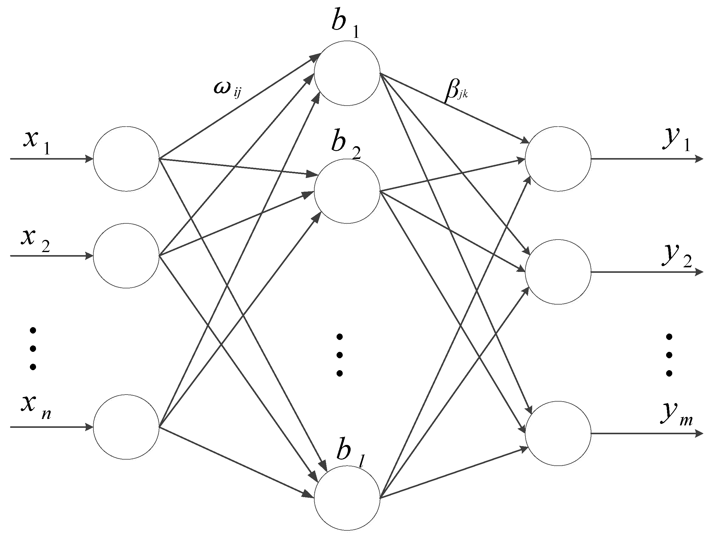
Extreme learning machine (ELM) is a new algorithm proposed by Huang et al. [37] for developing by single-hidden layer feedforward neural networks (SLFNs). ELM greatly improves the learning speed and generalization performance of the network, and overcomes these problems of local minimum, overfitting, and inappropriate choice of learning rate that are common in traditional gradient algorithms. In recent years, it has been widely used in time series prediction and has achieved good predictive effect [38]. The structure of typical SLFNs is shown in Figure 1.
The model consists of three layers, including an input layer, a hidden layer, and an output layer. The input layer and the hidden layer neurons, and the hidden layer and the output layer neurons are fully connected. Among them, the input layer has n neurons, that is, there are n input variables. The hidden layer has l neurons, the output layer has m neurons, that is, there are m output variables. Suppose there are N different random samples , where , , the SLFNs model for which the incentive function is can be expressed as:
where is the connection weight vector between the ith hidden layer neuron and the input layer neuron, and the connection weight vector between the ith hidden layer neuron and the output layer neuron is . is the threshold of the ith hidden layer and is the output value of the node.
The goal of SLFNs learning is to minimize the output error, which can be expressed as:
The parameters and satisfy the following formula:
and the above formula can be expressed as a matrix:
where H is the hidden layer output matrix of the neural network, and the specific form is as follows:
The connection weight vector can be obtained by solving the least squares solution of the following equation:
and the solution is:
where is the Moore–Penrose generalized inverse of matrix H.
The algorithm of ELM is as follows:
- Step 1:
- Determine the number of hidden layer neurons. Randomly initialize input layer weight and hidden layer threshold .
- Step 2:
- Calculate the hidden layer output matrix H.
- Step 3:
- Calculate the output weight .
Compared with the traditional neural network algorithm (such as BP neural network), ELM does not need to set a large number of network training parameters artificially. It only needs to set the number of hidden layer nodes and select the activation function type according to the problem to be solved. During the execution of the algorithm, there is no need to adjust input weight and hidden layer threshold, and a unique optimal solution is generated. Therefore, compared with the traditional gradient-based learning algorithm, ELM has the advantages of fast learning and good generalization performance. In the prediction field, it has also achieved better performance than BP neural network and radial basis function (RBF) neural network [39].
2.3. The Proposed Hybrid VMD-ELM Model
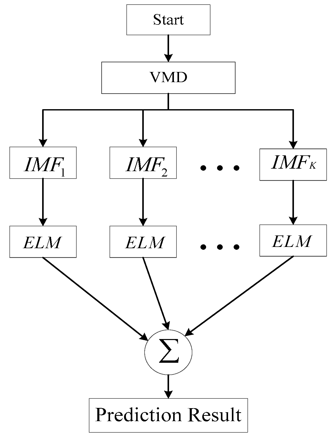
Since precipitation is affected by many factors, the precipitation time series has complicated nonlinear characteristics. Modeling with a single predictive model is difficult. Therefore, a hybrid forecasting model based on VMD and ELM is proposed to improve the prediction accuracy of monthly precipitation time series. The VMD algorithm is utilized to decompose the monthly precipitation time series into several relatively stable IMFs and reduce the difficulty of modeling. Then, the IMFs are easily predicted by using ELM. Finally, the predicted values of these components are aggregated as the final prediction results. Figure 2 clearly shows the workflow chart of the proposed hybrid VMD-ELM forecasting model in detail. The VMD-ELM model contains four main steps as follows:
- Step 1:
- Load the original data, and the data is decomposed into a set of IMFs by using VMD method.
- Step 2:
- Set up an ELM prediction model for each IMF. Divide the data of each IMF component into training samples and test samples and all samples are normalized.
- Step 3:
- Determine the number of input layers, output layers, and hidden layers of the ELM model.
- Step 4:
- The established ELM model is used to predict each IMF. The reconstructed IMFs are the final prediction results for the monthly precipitation time series.
3. Data Simulation and Analysis
3.1. Data Decomposition Preprocessing
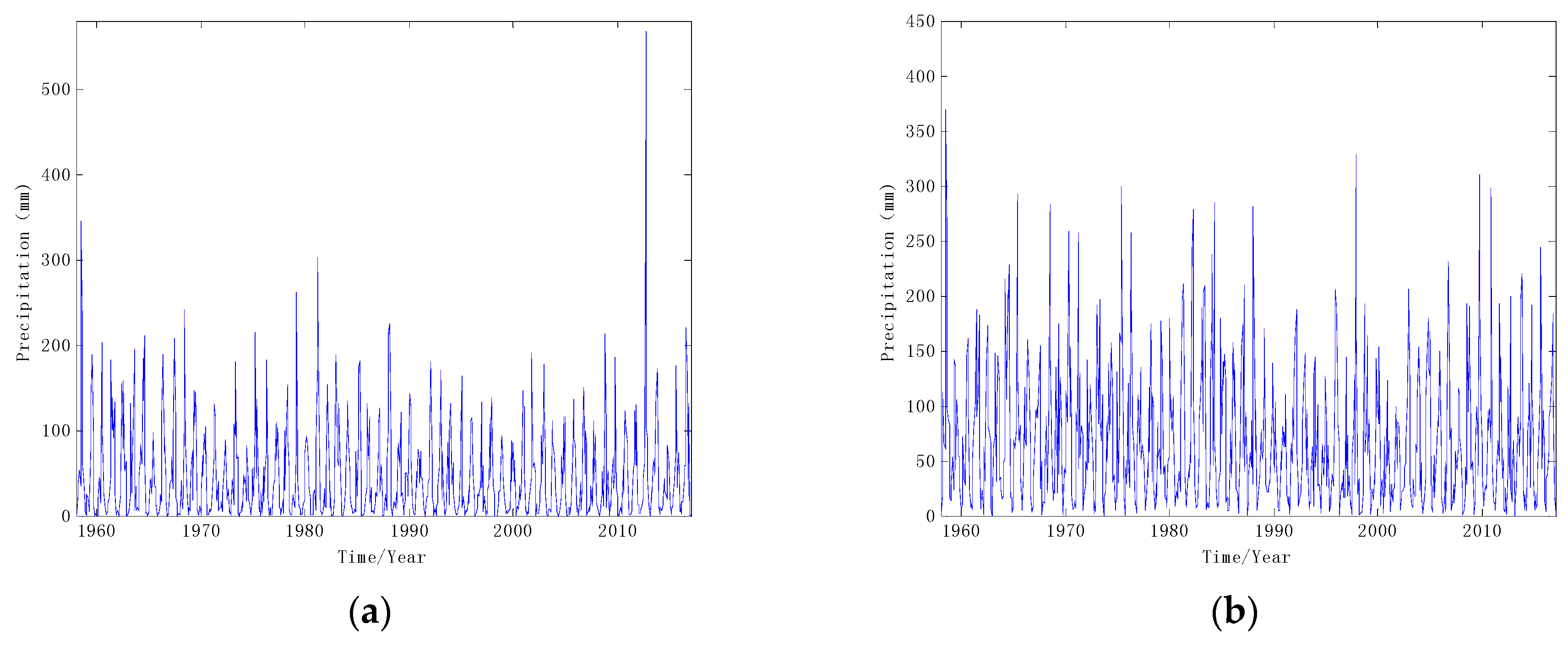
Shaanxi Province is located in the northwest of China, across the north temperate zone and subtropical zone, and it is a continental monsoon climate as a whole. Yan’an City is located in the southern half of Shaanxi Province. The landform is dominated by the loess plateau and hills. The area belongs to the plateau continental monsoon climate. The average annual precipitation is more than 500 mm, and the rainfall is unevenly distributed during the year. Precipitation is mainly concentrated from June to September. Huashan is located in Huayin City of Shaanxi Province. It was called “west high mountain” in ancient times and is one of the famous five high mountains in China. Huashan is far away from the ocean and lies between 30° and 60° in the north latitude of the west wind belt, which belongs to the warm temperate continental monsoon climate. The average annual precipitation has been about 900 mm for many years. This paper takes the monthly precipitation data of Yan’an and Huashan for a total of 60 years from 1958 to 2017. The data is from the China Meteorological Data Service Center (http://data.cma.cn/). The time series of monthly precipitation in the two places for 60 years are shown in Figure 3.
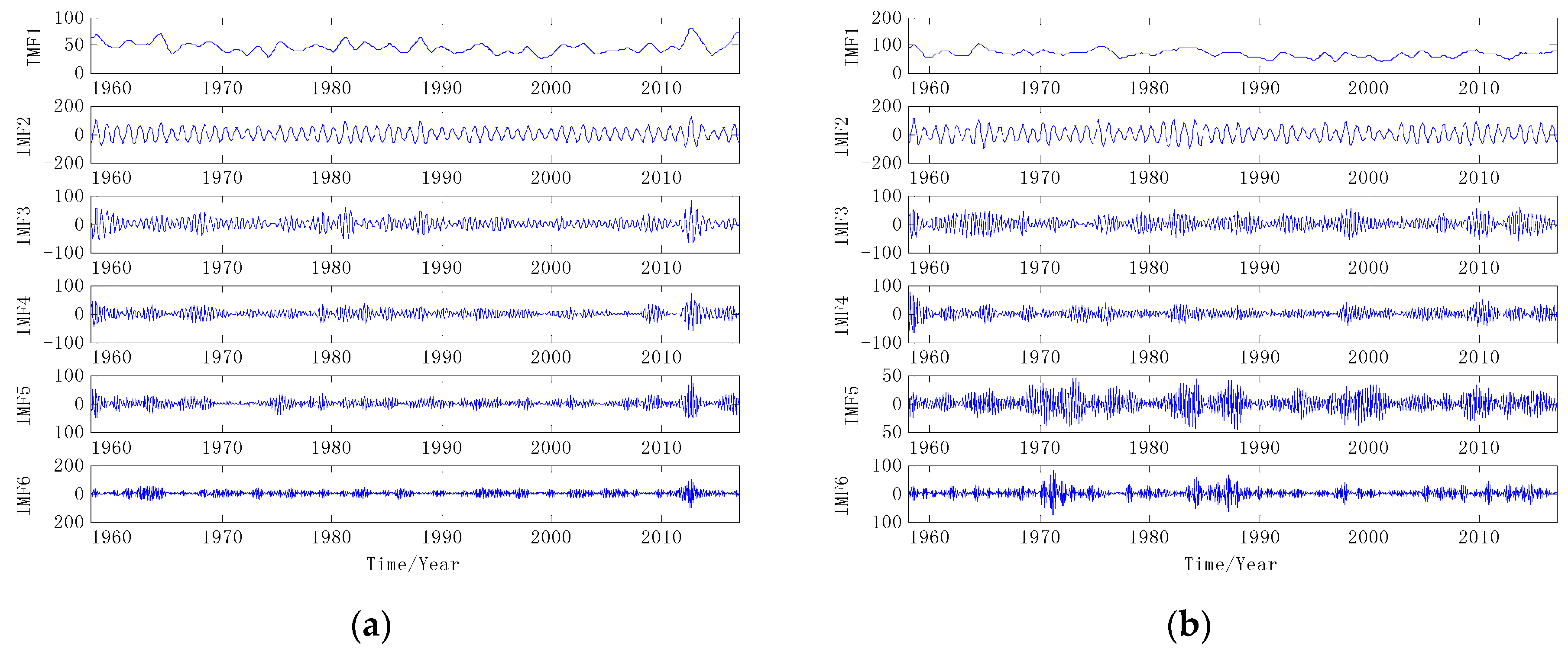
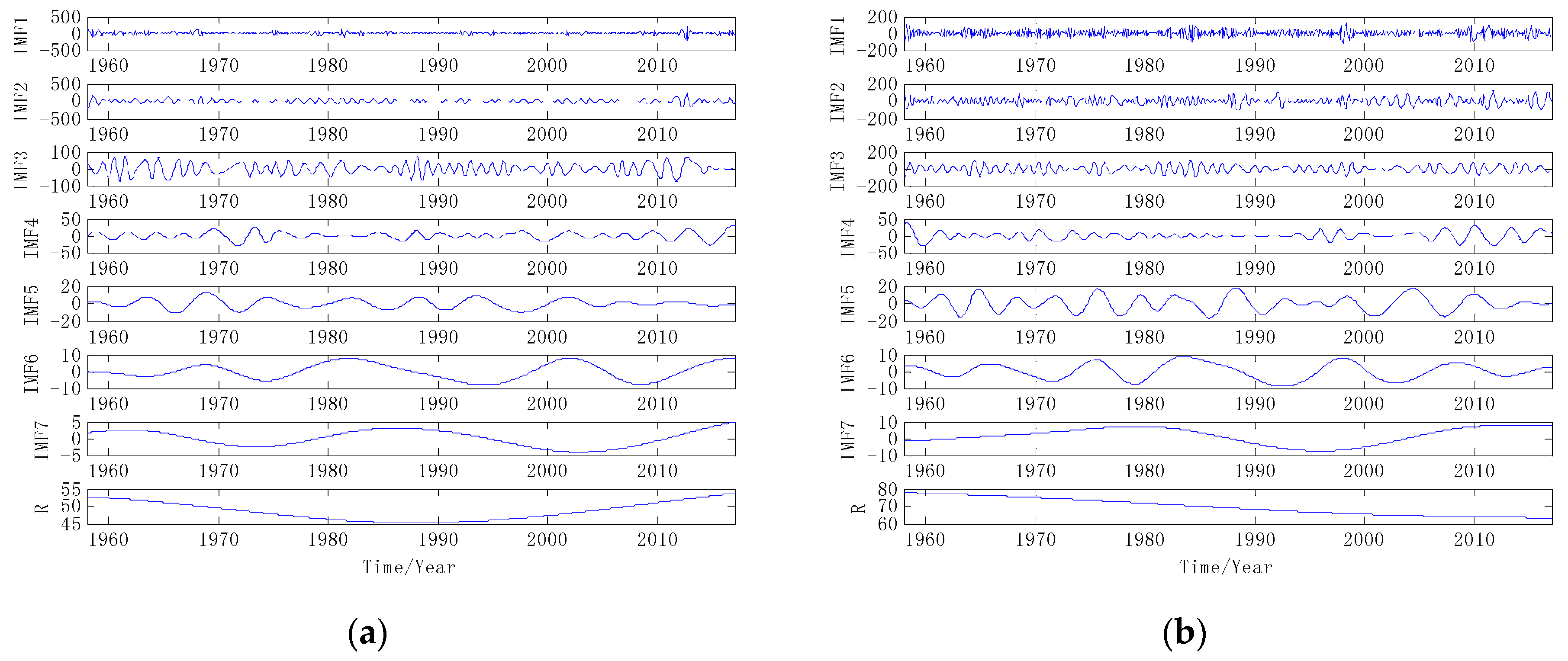
Given the nonlinearity of the monthly precipitation series, there will be a greater error with direct prediction. In order to improve the accuracy of prediction, the data complexity needs to be reduced. The original data is decomposed to several IMFs by using VMD. The number of IMFs K is set before proceeding with the VMD method. However, we can see from the previous test that for these two groups of precipitation time series, the following IMFs tend to be similar when K > 6, so we chose K = 6 in this paper. The results of VMD are shown in Figure 4. The same data samples are also decomposed by EMD as shown in Figure 5.
As shown in Figure 4 and Figure 5, two samples of precipitation time series are decomposed into 6 IMFs by VMD, and 7 IMFs and one remainder are obtained by EMD. From the decomposition results, it can be seen that the trend of the high frequency IMFs decomposed by the VMD method is relatively stable, which is conducive to prediction. Although the low-frequency component fluctuates greatly, the prediction error is limited. Because the final VMD forecast result is an accumulation of each IMF’s forecast result, the characteristics of the VMD result help to improve the prediction accuracy. However, end-point effects occur during the decomposition process of EMD. Large fluctuations occur at both ends of the IMF component and affect all IMFs continuously. As a result, the prediction result of EMD has a large error. Therefore, IMFs decomposed by VMD are more suitable for the establishment of hybrid forecasting model than IMFs decomposed by EMD [40].
3.2. Performance Standards of Prediction Accuracy
This study uses the following three error indicators to evaluate the performance of the proposed hybrid prediction model: mean absolute error (MAE), root mean squared error (RMSE), and mean absolute percentage error (MAPE). The error of prediction value is quantified by using the performance indexes of MAE, RMSE, and MAPE. The smaller the value, the better the prediction accuracy. These formulas are as follows:
where is forecast data, is original data.
3.3. Component Prediction and Reconstruction
There are a total of 720 values for monthly precipitation data from 1958 to 2017. After the decomposition of the original monthly precipitation time series into 6 IMFs by employing the VMD method, we use the ELM model to train and predict each IMF component. The number of nodes in the input layer is 5, the number of nodes in the hidden layer is 15, and the number of nodes in the output layer is 1. The first five values of each IMF component are used to predict the sixth value. 720 values can be divided into 715 sets of data, where the former 667 sets of data are used as the train data, and the latter 48 sets of data are used as the forecast data. Activation function is radial basis function. Before training the ELM model, all the values of IMFs are normalized to improve the efficiency of the ELM model. The normalization formula is defined as follows:
where is the normalized data, is the original data, is the maximum value, and is the minimum value.
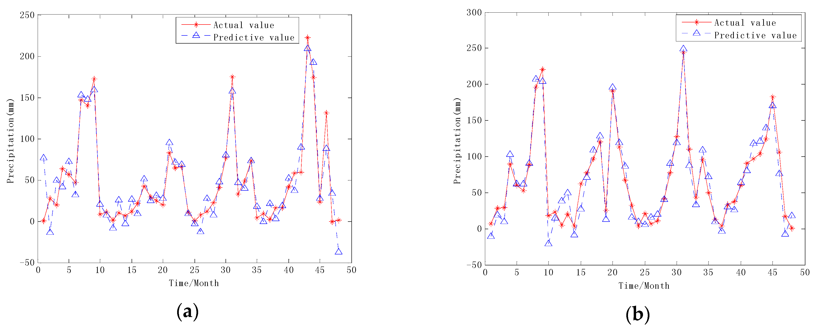
The ELM prediction model is established for each IMF, and the predicted values of each IMF component are reconstructed as the final prediction results of the hybrid VMD-ELM model. The prediction results are as shown in Figure 6.
As can be seen from Figure 6, the red line represents the actual monthly precipitation data, and the blue line represents the predicted value of the combined forecast model. It can be seen that the VMD-ELM model proposed in this paper is good for fitting the original data and can predict the monthly precipitation in Yan’an and Huashan very well.
3.4. Results Analysis and Performance Comparison
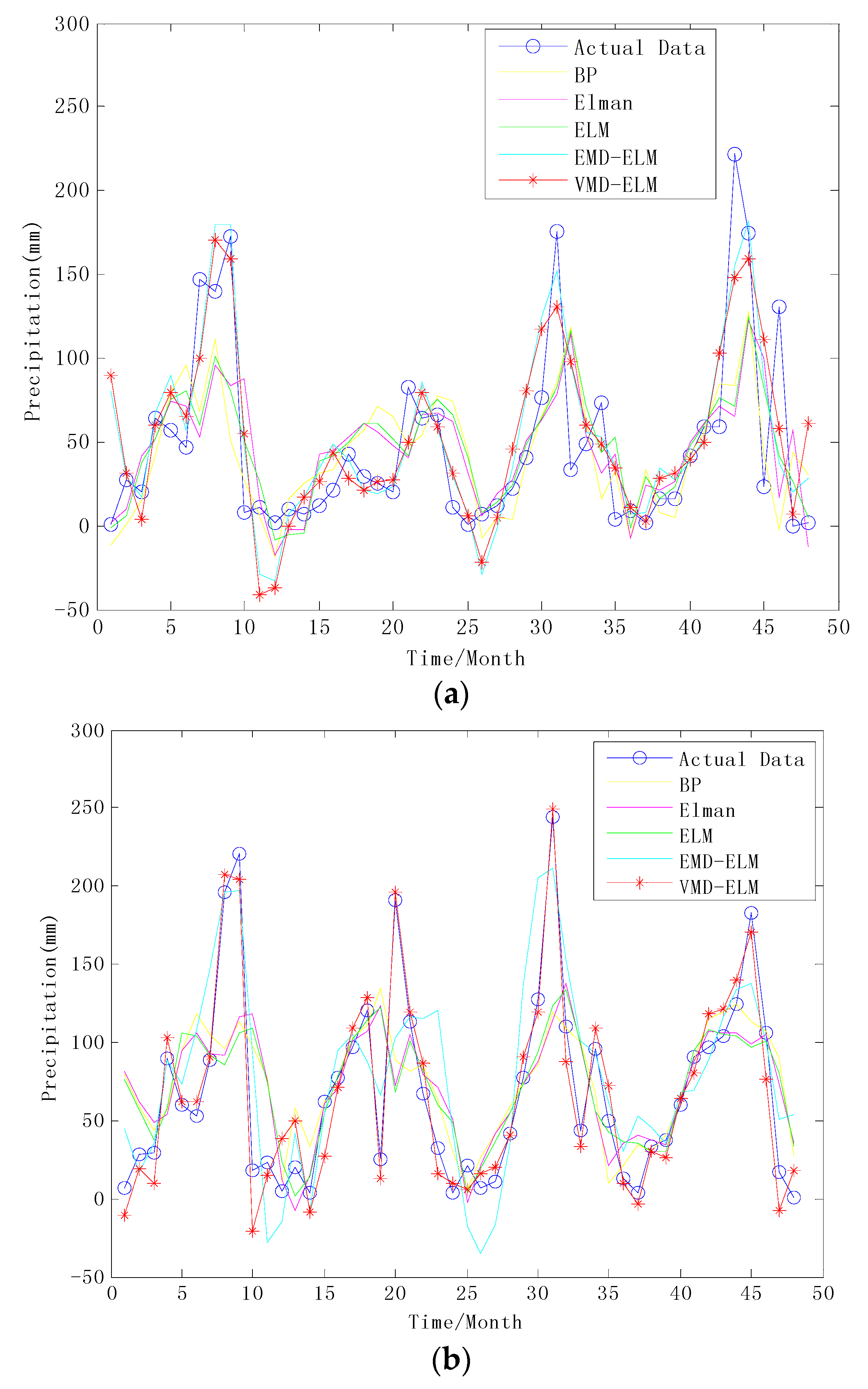
For comparison purposes, all data samples are applied to the BP model, Elman model, ELM model, and EMD-ELM model in this paper, and the predicted results of the hybrid VMD-ELM model are compared with other models. The predicted results of all models are illustrated in Figure 7. It can be seen from Figure 7 that each model gives different forecast results for the two monthly precipitation time series. It is evident that the BP model, compared to the other models, gives the worst results for the Yan’an and Huashan, and the prediction effect of a single ELM model is somewhat better than that of the BP model. The hybrid EMD-ELM and VMD-ELM models perform better than the single BP, Elman, and ELM models for the two cases. Moreover, the predictive effect of VMD-ELM is significantly better than that of EMD-ELM, especially in the prediction of Huashan monthly precipitation time series. The performance index values of each model are intuitively given in Table 1.
From Table 1, it can be seen that the BP model has the worst prediction results, which is the reason for the inherent drawback itself. Moreover, the ELM model improves the slow learning speed of the BP neural network and defects of easily falling into the local minimum, and the error performance values are less than for the BP model. Furthermore, the prediction effects of the two hybrid models, EMD-ELM and VMD-ELM, are better than those of the other single models, especially for VMD-ELM, which is the best. The hybrid VMD-ELM model achieves smaller MAE, RMSE, and MAPE values than the other four models for monthly precipitation time series in Yan’an and Huashan. Thus, the proposed hybrid model can predict the variation trend of the monthly precipitation time series well, which shows it is a good prediction model.
4. Conclusions
The reliable and accurate estimation of precipitation trends is essential in order to manage water resources and carry out hydrological forecasts. In this paper, a hybrid forecasting model based on VMD and ELM is proposed and applied to the prediction of monthly precipitation in Yan’an and Huashan. The original data are decomposed into several relatively stable IMFs by using VMD, and then each IMF is predicted by the ELM model. Finally, the predicted results of each IMF component are aggregated as the final prediction results. The three performance indicators MAE, RMSE, and MAPE are employed to measure the prediction accuracy of BP, Elman, ELM, EMD-ELM, and VMD-ELM models. Based on analysis of the research results, the MAE, RMSE, and MAPE values of the hybrid VMD-ELM forecasting model proposed in this paper are the smallest. In other words, compared with other models, the hybrid model improves the prediction accuracy and reduces errors.
The hybrid VMD-ELM prediction model proposed in this paper can effectively improve the accuracy of precipitation forecasting, and it has the following advantages: (a) VMD is used to decompose the original data, and it has solved the problems of mode mixing and end-point effects in the EMD process, reduced the data complexity, and facilitated the prediction modeling. (b) ELM has greatly improved the defects of the traditional algorithms, such as slow training speed and ease of falling into local minimum, and it has good generalization performance. (c) The hybrid VME-ELM model is first used to forecast monthly precipitation. Through the study and analysis of the monthly precipitation cases in Yan’an and Huashan over the past 60 years, it is shown that the prediction results of the hybrid model are more accurate. The results from this research will be beneficial for sustainable water resource management. Of course, it also has a good reference value for forecasting actual problems accurately, such as short-time traffic flow and other time series.
Author Contributions
G.L., X.M. and H.Y. conceived the idea and research theme. X.M. designed and performed the experiments. G.L., X.M. and H.Y. analyzed the experimental results. G.L., X.M. and H.Y. wrote and revised the paper.
Funding
This work was supported by the National Natural Science Foundation of China (No. 51709228).
Conflicts of Interest
The authors declare no conflict of interest.
References
- Xu, X.C.; Zhang, X.Z.; Dai, E.F.; Song, W. Research of trend variability of precipitation intensity and their contribution to precipitation in China from 1961 to 2010. Geogr. Res. 2014, 33, 1335–1347. [Google Scholar] [CrossRef]
- Huang, X.Y.; Li, Y.H.; Feng, J.Y.; Wang, J.S.; Wang, Z.L.; Wang, S.J.; Zhang, Y. Climate characteristics of precipitation and extreme drought events in northwest China. Acta Ecol. Sin. 2015, 35, 1359–1370. [Google Scholar] [CrossRef]
- Jin, L.Y.; Fu, J.L.; Chen, F.H. Spatial differences of precipitation over northwest China during the last 44 years and its response to global warming. Sci. Geogr. Sin. 2005, 25, 567–572. [Google Scholar] [CrossRef]
- Wu, C.L.; Chau, K.W.; Fan, C. Prediction of rainfall time series using modular artificial neural networks coupled with data-preprocessing techniques. J. Hydrol. 2010, 389, 146–167. [Google Scholar] [CrossRef] [Green Version]
- Jiao, G.M.; Guo, T.L.; Ding, Y.J. A new hybrid forecasting approach applied to hydrological data: A case study on precipitation in Northwestern China. Water 2016, 8, 367. [Google Scholar] [CrossRef]
- Ma, Z.Q.; Xu, M.X.; Yu, W.Y.; Wen, S.Y. Statistic Markovian model for predicting of annual precipitation. J. Nat. Resour. 2010, 25, 1033–1041. [Google Scholar]
- Qian, J.Z.; Zhu, X.Y.; Wu, J.F. Time Series-Markov prediction model for precipitation in the course of evaluation of groundwater resources. Sci. Geogr. Sin. 2001, 21, 350–353. [Google Scholar] [CrossRef]
- Zhang, X.; Ren, Y.T.; Wang, F.L.; Fu, Q. Prediction of annual precipitation based on improved Grey Markov model. Math. Pract. Theory 2011, 41, 51–57. [Google Scholar]
- Li, C.Y.; Gu, Y.G. Application of Grey forecasting model to area rainfall prediction in upstream of Chanjiang River. Meteorol. Sci. Technol. 2003, 31, 223–225. [Google Scholar] [CrossRef]
- Chi, D.C.; Zhang, T.N.; Wu, X.M.; Zhang, L.F. Application of ARMA model in the annual precipitation forecast of Taizi River. J. Shenyang Agric. Univ. 2012, 43, 607–610. [Google Scholar] [CrossRef]
- Yang, Q.M. Extended complex autoregressive model of low-frequency rainfalls over the lower reaches of Yangtze River valley for extended range forecast in 2013. Acta Phys. Sin. 2014, 63. [Google Scholar] [CrossRef]
- Huang, H.; Cai, R.; Aili, N.; Mu, Z.X. Coupling prediction for annual precipitation in Xinjiang based on ARIMA and GA-Elman neural network. Xinjiang Agric. Sci. 2015, 52, 1093–1098. [Google Scholar] [CrossRef]
- Liu, L.; Ye, W. Precipitation prediction of time series model based on BP artificial neural network. J. Water Resour. Water Eng. 2010, 21, 156–159. [Google Scholar]
- Hartmann, H.; Becker, S.; King, L. Predicting summer rainfall in the Yangtze River basin with neural networks. Int. J. Climatol. 2010, 28, 925–936. [Google Scholar] [CrossRef]
- Ramana, R.V. Monthly rainfall prediction using wavelet neural network analysis. Water Resour. Manag. 2013, 27, 3697–3711. [Google Scholar] [CrossRef]
- Xie, Y.H.; Zhang, M.M.; Yang, L.; Zhang, H.D. Predicting urban PM2.5 concentration in China Using support vector regression. Comput. Eng. Des. 2015, 36, 3106–3111. [Google Scholar] [CrossRef]
- Zou, W.D.; Zhang, B.H.; Yao, F.X.; He, C.X. Verification and forecasting of temperature and humidity in solar greenhouse based on improved extreme learning machine algorithm. Trans. Chin. Soc. Agric. Eng. 2015, 31, 194–200. [Google Scholar] [CrossRef]
- Li, Y.B.; You, F.; Huang, Q.; Xu, J.X. Least squares support vector machine model of multivariable prediction of stream flow. J. Hydroelectr. Eng. 2010, 29, 28–33. [Google Scholar]
- Niu, W.J.; Feng, Z.K.; Cheng, C.T.; Zhou, J.Z. Forecasting Daily Runoff by Extreme Learning Machine Based on Quantum-Behaved Particle Swarm Optimization. J. Hydrol. Eng. 2018, 23. [Google Scholar] [CrossRef]
- Xu, S.L.; Niu, R.Q. Displacement prediction of Baijiabao landslide based on empirical mode decomposition and long short-term memory neural network in Three Gorges area, China. Comput. Geosci. 2018, 111, 87–96. [Google Scholar] [CrossRef]
- Zhu, B.X.; Han, D.; Wang, P.; Wu, Z.C.; Zhang, T.; Wei, Y.M. Forecasting carbon price using empirical mode decomposition and evolutionary least squares support vector regression. Appl. Energy 2017, 191, 521–530. [Google Scholar] [CrossRef]
- Xiao, Y.; Yin, F.L. Decorrelation EMD: A new method to eliminating mode mixing. J. Vib. Shock 2015, 34, 25–29. [Google Scholar] [CrossRef]
- Wu, Z.H.; Huang, N.E. Ensemble empirical mode decomposition: A noise-assisted data analysis method. Adv. Adapt. Data Anal. 2009, 1, 1–41. [Google Scholar] [CrossRef]
- Dragomiretskiy, K.; Zosso, D. Variational mode decomposition. IEEE Trans. Signal Process. 2014, 62, 531–544. [Google Scholar] [CrossRef]
- Lahmiri, S. Intraday stock price forecasting based on variational mode decomposition. J. Comput. Sci. 2016, 12, 23–27. [Google Scholar] [CrossRef]
- Liang, Z.; Sun, G.Q.; Li, H.C.; Wei, Z.N.; Zang, H.Y.; Zhou, Y.Z.; Chen, S. Short-term load forecasting based on VMD and PSO optimized deep belief network. Power Syst. Technol. 2018, 42, 598–606. [Google Scholar] [CrossRef]
- Zhang, D.Y.; Wu, X.T.; Yuan, X.H.; Yuan, Y.B.; Xu, H.P. Prediction of solar irradiation based on improved LSSVM model. Water Resour. Power 2017, 35, 205–208. [Google Scholar]
- Li, K.; Su, L.; Wu, J.; Wang, H.; Chen, P. A Rolling Bearing Fault Diagnosis Method Based on Variational Mode Decomposition and an Improved Kernel Extreme Learning Machine. Appl. Sci. 2017, 7, 1004. [Google Scholar] [CrossRef]
- Liu, C.L.; Wu, Y.J.; Zhen, C.G. Rolling bearing fault diagnosis based on variational mode decomposition and fuzzy C means clustering. Proc. Chin. Soc. Electr. Eng. 2015, 35, 3358–3365. [Google Scholar] [CrossRef]
- Cai, W.N.; Yang, Z.J.; Wang, Z.J.; Wang, Y.L. A new compound fault feature extraction method based on multipoint kurtosis and variational mode decomposition. Entropy 2018, 7, 521. [Google Scholar] [CrossRef]
- Li, Y.X.; Li, Y.A.; Chen, X.; Yu, J. Denoising and Feature Extraction Algorithms Using NPE Combined with VMD and Their Applications in Ship-Radiated Noise. Symmetry 2017, 9, 256. [Google Scholar] [CrossRef]
- Wang, S.X.; Wang, Y.W.; Liu, Y.; Zhang, N. Hourly solar radiation forecasting based on EMD and ELM neural network. Electr. Power Autom. Equip. 2014, 34, 7–12. [Google Scholar] [CrossRef]
- Niu, M.F.; Gan, K.; Sun, S.L.; Li, F.Y. Application of decomposition-ensemble learning paradigm with phase space reconstruction for day-ahead PM2.5 concentration forecasting. J. Environ. Manag. 2017, 196, 110–118. [Google Scholar] [CrossRef] [PubMed]
- Zhang, X.K.; Zhang, Q.W.; Zhang, G.; Nie, Z.N.; Gui, Z.F. A hybrid model for annual runoff time series forecasting using Elman neural network with ensemble empirical mode decomposition. Water 2018, 10, 416. [Google Scholar] [CrossRef]
- Fan, L.; Wei, Z.N.; Li, H.J.; Kwork, W.C.; Sun, G.Q.; Sun, Y.H. Short-term wind speed interval prediction based on VMD and BA-RVM algorithm. Electr. Power Autom. Equip. 2017, 37, 93–100. [Google Scholar] [CrossRef]
- Sun, G.; Chen, T.; Wei, Z.N.; Sun, Y.H.; Zang, H.X.; Chen, S. A carbon price forecasting model based on variational mode decomposition and spiking neural networks. Energies 2016, 9, 54. [Google Scholar] [CrossRef]
- Huang, G.B.; Qin, Y.Z.; Chee, K.S. Extreme learning machine: Theory and applications. Neurocomputing 2006, 70, 489–501. [Google Scholar] [CrossRef] [Green Version]
- Lian, C.; Zeng, Z.G.; Yao, W.; Tang, H.M. Ensemble of extreme learning machine for landslide displacement prediction based on time series analysis. Neural Comput. Appl. 2014, 24, 99–107. [Google Scholar] [CrossRef]
- Cui, D.W. Application of extreme learning machine to total phosphorus and total nitrogen forecast in lakes and reservoirs. Water Resour. Prot. 2013, 29, 61–66. [Google Scholar] [CrossRef]
- Naik, J.; Dash, S.; Dash, P.K.; Bisos, R. Short Term Wind Power Forecasting using Hybrid Variational Mode Decomposition and Multi-Kernel Regularized Pseudo Inverse Neural Network. Renew. Energy 2018, 118, 180–212. [Google Scholar] [CrossRef]
Figure 1.
The structure of typical SLFNs.

Figure 2.
The flowchart of VMD-ELM prediction model.

Figure 3.
Monthly Precipitation Time Series from 1958 to 2017 of (a) Yan’an; (b) Huashan.

Figure 4.
The results of VMD method (a) Yan’an; (b) Huashan.

Figure 5.
The results of EMD method (a) Yan’an; (b) Huashan.

Figure 6.
The monthly precipitation time series prediction results of hybrid VMD-ELM model. (a) Yan’an; (b) Huashan.
Figure 6.
The monthly precipitation time series prediction results of hybrid VMD-ELM model. (a) Yan’an; (b) Huashan.

Figure 7.
Performance comparison of the prediction results of monthly precipitation for the BP, Elman, ELM, EMD-ELM, and VMD-ELM models. (a) Yan’an; (b) Huashan.
Figure 7.
Performance comparison of the prediction results of monthly precipitation for the BP, Elman, ELM, EMD-ELM, and VMD-ELM models. (a) Yan’an; (b) Huashan.


Table 1.
Predictive performance comparison of each model.
| Place | Models | Error Indicators | ||
|---|---|---|---|---|
| MAE | RMSE | MAPE | ||
| Yan’an | BP | 33.0841 | 49.7006 | 3.3536 |
| Elman | 32.7371 | 47.2576 | 2.7936 | |
| ELM | 30.5377 | 43.6451 | 2.7622 | |
| EMD-ELM | 24.4135 | 32.7755 | 2.1972 | |
| VMD-ELM | 15.2966 | 20.3605 | 1.7217 | |
| Huashan | BP | 37.4068 | 50.8760 | 4.3309 |
| Elman | 35.3464 | 49.2296 | 4.1087 | |
| ELM | 34.2236 | 48.6962 | 3.7824 | |
| EMD-ELM | 29.3452 | 38.2472 | 3.1507 | |
| VMD-ELM | 13.5179 | 16.7612 | 1.9101 | |
© 2018 by the authors. Licensee MDPI, Basel, Switzerland. This article is an open access article distributed under the terms and conditions of the Creative Commons Attribution (CC BY) license (http://creativecommons.org/licenses/by/4.0/).
Share and Cite
MDPI and ACS Style
Li, G.; Ma, X.; Yang, H. A Hybrid Model for Monthly Precipitation Time Series Forecasting Based on Variational Mode Decomposition with Extreme Learning Machine. Information 2018, 9, 177. https://doi.org/10.3390/info9070177
AMA Style
Li G, Ma X, Yang H. A Hybrid Model for Monthly Precipitation Time Series Forecasting Based on Variational Mode Decomposition with Extreme Learning Machine. Information. 2018; 9(7):177. https://doi.org/10.3390/info9070177
Chicago/Turabian StyleLi, Guohui, Xiao Ma, and Hong Yang. 2018. "A Hybrid Model for Monthly Precipitation Time Series Forecasting Based on Variational Mode Decomposition with Extreme Learning Machine" Information 9, no. 7: 177. https://doi.org/10.3390/info9070177
Note that from the first issue of 2016, this journal uses article numbers instead of page numbers. See further details here.