Apple Image Recognition Multi-Objective Method Based on the Adaptive Harmony Search Algorithm with Simulation and Creation


1
College of Information Science and Technology, Gansu Agricultural University, Lanzhou 730070, China
2
School of Electronic and Information Engineering, Lanzhou Jiaotong University, Lanzhou 730070, China
*
Author to whom correspondence should be addressed.
Information 2018, 9(7), 180; https://doi.org/10.3390/info9070180
Submission received: 29 June 2018
/
Revised: 17 July 2018
/
Accepted: 18 July 2018
/
Published: 20 July 2018
Abstract
:Aiming at the low recognition effect of apple images captured in a natural scene, and the problem that the OTSU algorithm has a single threshold, lack of adaptability, easily caused noise interference, and over-segmentation, an apple image recognition multi-objective method based on the adaptive harmony search algorithm with simulation and creation is proposed in this paper. The new adaptive harmony search algorithm with simulation and creation expands the search space to maintain the diversity of the solution and accelerates the convergence of the algorithm. In the search process, the harmony tone simulation operator is used to make each harmony tone evolve towards the optimal harmony individual direction to ensure the global search ability of the algorithm. Despite no improvement in the evolution, the harmony tone creation operator is used to make each harmony tone to stay away from the current optimal harmony individual for extending the search space to maintain the diversity of solutions. The adaptive factor of the harmony tone was used to restrain random searching of the two operators to accelerate the convergence ability of the algorithm. The multi-objective optimization recognition method transforms the apple image recognition problem collected in the natural scene into a multi-objective optimization problem, and uses the new adaptive harmony search algorithm with simulation and creation as the image threshold search strategy. The maximum class variance and maximum entropy are chosen as the objective functions of the multi-objective optimization problem. Compared with HS, HIS, GHS, and SGHS algorithms, the experimental results showed that the improved algorithm has higher a convergence speed and accuracy, and maintains optimal performance in high-dimensional, large-scale harmony memory. The proposed multi-objective optimization recognition method obtains a set of non-dominated threshold solution sets, which is more flexible than the OTSU algorithm in the opportunity of threshold selection. The selected threshold has better adaptive characteristics and has good image segmentation results.
1. Introduction
The harmony search (HS) algorithm [1] is a swarm intelligence algorithm that simulates the process of music players’ repeated tuning of the pitch of each musical instrument through memory to achieve a wonderful harmony process. It has been successfully applied to many engineering problems. Like other swarm intelligence algorithms, the HS algorithm also has problems with premature convergence and stagnant convergence [2,3]. In recent years, scholars have made many improvements to the optimization performance of the HS algorithm, such as the probabilistic idea of applying the distributed estimation algorithm in the [2] to design an adaptive adjustment strategy and improve the search ability of the algorithm. In [3], the HS algorithm and the genetic algorithm (GA) are combined to obtain a better initial solution based on multiple iterations of the genetic algorithm, and then the harmony search algorithm is used to further search for possible solutions in the adjacent region. Zhu et al. linearly combines the optimal harmony vector with the two harmony vectors randomly selected in the population to generate a new harmony and expand the local search area [4]. Wu et al. uses the competitive elimination mechanism to update the harmony memory library to accelerate the process of survival of the fittest. Some studies have designed two key parameters of the HS algorithm to overcome the shortcomings of fixed parameters [5]. These two parameters also have improved from different perspectives and proposed different improved harmony search algorithms in [6,7,8]. The studies in [9,10] apply the improved HS algorithm to multi-objective optimization problems.
Relevant scholars have conducted a large number of basic studies on the HS algorithm, and proposed improvements, achieving good results in application. Simulated annealing and a genetic algorithm are used to optimally adjust the weights for the aggregation mechanism [11]. An innovative tuning approach for fuzzy control systems (CSs) with a reduced parametric sensitivity using the grey wolf optimizer (GWO) algorithm was proposed in [12]. The GWO algorithm is used in solving the optimization problems, where the objective functions include the output sensitivity functions [12]. Echo state networks (ESN) are a special form of recurrent neural networks (RNNs), which allow for the black box modeling of nonlinear dynamical systems. The harmony search (HS) algorithm shows good performance, proposed for training the echo state network in an online manner [13]. The design of the Takagi–Sugeno fuzzy controllers in state feedback formed using swarm intelligence optimization algorithms was proposed in [14], and the particle swarm optimization, simulated annealing and gravitational search algorithms are adopted. In terms of image applications of HS, the following studies have been conducted. A novel approach to visual tracking called the harmony filter is presented. The harmony filter models the target as a color histogram and searches for the best estimated target location using the Bhattacharyya coefficient as a fitness metric [15]. In [16], a new dynamic clustering algorithm based on the hybridization of harmony search (HS) and fuzzy c-means to automatically segment MRI brain images in an intelligent manner was presented. Improvements to Harmony Search (HS) in circle detection was proposed that enables the algorithm to robustly find multiple circles in larger data sets and still work on realistic images that are heavily corrupted by noisy edges [17]. A new approach to estimate the vanishing point using a harmony search (HS) algorithm was proposed in [18]. In the theoretical background of HS, the following studies have been conducted. In order to consider the realistic design situations, a novel derivative for discrete design variables based on a harmony search algorithm was proposed in [19]. In [20], it presents a simple mathematical analysis of the explorative search behavior of harmony search (HS) algorithm. The comparison of the final designs of conventional methods and metaheuristic based structural optimization methods was discussed in [21]. In the improvement of adaptive methods of HS, the following studies have been conducted. An adaptive harmony search algorithm was proposed for solving structural optimization problems to incorporate a new approach for adjusting these parameters automatically during the search for the most efficient optimization process [22]. A novel technique to eliminate tedious and experience-requiring parameter assigning efforts was proposed for the harmony search algorithm in [23]. Pan et al. presents a self-adaptive global best harmony search (SGHS) algorithm for solving continuous optimization problems [24].
Recognition of apple images is one of the most basic aspects of computer processing apple grading [25]. Apple image recognition refers to the separation of apple fruit from branches, leaves, soil, and sky, i.e., image segmentation techniques [26]. The threshold segmentation method is an extremely important and widely used image segmentation method [27]. Among them, the maximum class variance (OTSU) [28] and maximum entropy method [29] are the two most commonly used threshold segmentation methods. Both types of segmentation methods have different degrees of defects [30]. The classical OTSU algorithm has the problem that the ideal segmentation effect cannot be obtained for complex images of natural scenes [30]. Although the OTSU algorithm solves the problem of threshold selection, it has the problems of lacking adaptability, easily causes noise interference and over-segmentation, and requires a great deal of time for computing, and so on. Therefore, the classical OTSU algorithm still needs further improvement. In order to comprehensively utilize the advantages of the two segmentation methods, a multi-objective optimization problem is introduced. In recent years, the HS algorithm has made some progress in solving multi-objective optimization problems, such as the stand-alone scheduling problem [10], the wireless sensor network routing problem [31], the urban one-way traffic organization optimization problem [32], and the distribution network model problem [33]. In [34], the study employed a phenomenon-mimicking algorithm and harmony search to perform the bi-objective trade-off. The harmony search algorithm explored only a small amount of total solution space in order to solve this combinatorial optimization problem. A multi-objective optimization model based on the harmony search algorithm (HS) was presented to minimize the life cycle cost (LCC) and carbon dioxide equivalent (CO2-eq) emissions of the buildings [35]. A novel fuzzy-based velocity reliability index using fuzzy theory and harmony search was proposed, which is to be maximized while the design cost is simultaneously minimized [36]. These studies are closely integrated with specific application issues and cannot be easily extended to other application areas.
This paper proposes an apple image recognition multi-objective method based on the adaptive harmony search algorithm with simulation and creation (ARMM-AHS). This method transforms the image segmentation problem of natural scenes into a multi-objective optimization problem. It takes the maximum class variance and maximum entropy as the two objective functions of the optimization problem. A new adaptive harmony search algorithm with simulation and creation (SC-AHS) is proposed as a strategy for the image threshold search to achieve natural scene apple image segmentation. The results showed that the SC-AHS algorithm improves the global search ability and the diversity of the solution of the HS algorithm, and has obvious performance advantages of fast convergence. The ARMM-AHS method can effectively segment the apple image.
2. Theory Basis
2.1. Threshold Segmentation Principle of the OTSU Algorithm
The OTSU algorithm is a global threshold selection method. The basic idea is to use the grayscale histogram of the image to dynamically determine the segmentation threshold of the image with the maximum variance of the target and the background.
Suppose that the gray level of an apple image is the gray value of each pixel is , the number of pixels with gray value is , the total number of pixels in the image is , and the probability of gray value is set to .
Let the threshold divide the image into two classes and (target and background), that is, and respectively correspond to pixels with gray levels and , then the variance between the two classes is as shown in Equation (1):
The optimal threshold should maximize the variance between classes, which is an optimization problem, as shown in Equation (2):
Among them, and respectively represent the probability of the occurrence of class and class . and represent the average gray value of the class and class , respectively. represents the average gray level of the entire image. Therefore, the larger the value of , the better the threshold that is selected.
2.2. Maximum Entropy Segmentation Principle
For the same image, let us assume that the threshold t divides the image into two classes and . The probability distribution of the class is , and the probability distribution of the class is , where .
The entropy formula is as shown in Equation (3):
The optimal threshold should maximize the entropy, which is also an optimization problem, as shown in Equation (4).
3. Adaptive Harmony Search Algorithm with Simulation and Creation
The inertial particle and fuzzy reasoning were introduced into the bird swarm optimization algorithm (BSA) in [37] to make those birds that are foraging jump out of the local optimal solution to enhance the ability of global optimization. The fast shuffled frog leaping algorithm (FSFLA) proposed in [38] makes each frog individual evolve toward the best individual, which accelerates the individual evolutionary speed and improves the search speed of the algorithm. According to the no-free lunch theorem [39], this paper fuses the ideas of the above two different types of optimization algorithms’ mechanisms and proposes an adaptive harmony search algorithm with simulation and creation (SC-AHS) to improve the HS algorithm optimization performance.
3.1. Theory Basis
3.1.1. Adaptive Factor of Harmony Tone
Definition 1 (Adaptive factor of harmony tone).
Randomly generate Harmony Memory whose Size is HMS to find out the global optimal harmony, current optimal harmony, and global worst harmonyin each creation of the harmony memory. The adaptive factor of the harmony toneis defined as follows, and it is used to suppress randomness during simulation and creation of harmony tone:
3.1.2. Harmony Tone Simulation Operator
Definition 2 (Harmony tone simulation operator).
In one harmony evolution, each tone componentof each harmonyin the harmony memory adaptively evolves through the harmony tone simulation operator, as follows, to adjust the harmony individuals to evolve to optimal harmony individuals:
3.1.3. Harmony Tone Creation Operator
Definition 3 (Harmony tone creation operator).
In one harmony evolution, each tone componentof each harmonyin the harmony memory adaptively evolves through the harmony tone creation operator, as follows, to adjust harmony individuals away from the current optimal harmony individual evolution:
3.2. Adaptive Evolution Theorem with Simulation and Creation
Theorem 1 (Adaptive evolution theorem with simulation and creation).
In one harmony evolution, each tone componentin each harmonyin the harmony memory adaptively evolves through the harmony tone simulation operator according to the Equation (6). If, replacewith, respectively. Otherwise, it evolves through the harmony tone creation operator according to the Equation (7). Ifstill exists, use Equation (8) to randomly generate the harmony tone:
3.3. SC-AHS Algorithm Process
| Algorithm 1. SC-AHS |
| Input: the maximum number of evolutions , the size of the harmony memory HMS, the number of tone component N. |
| Output: global optimal harmony . |
| Step1: Randomly generate initial harmony individuals which number is HMS, marked as . The harmony memory is initialized according to Equation (1). The fitness of is . |
| Step2: Each tone component of each harmony is updated. |
| Begin |
| Sort each harmony by fitness in descending order to determine , and . |
| For () |
| Begin |
| Calculated according to Equation (5) |
| For () |
| Update according to Equation (6) to perform harmony tone simulation |
| End |
| if () |
| For ()
|
| End |
| else |
| For () |
| Update according to Equation (7) to perform harmony tone creation |
| End |
| If () |
| For ()
|
| End |
| else |
| For () |
| Randomly generate harmony tone according to Equation (8). |
| End |
| End |
| End |
| Step3: Determine if the number of evolutions has been reached . If not, go to Step 2. Otherwise, the algorithm stops and outputs . |
3.4. Efficiency Analysis of SC-AHS
The efficiency analysis of the algorithm shows that the time complexity of the HS algorithm is , and the space complexity is , while the time complexity of the SC-AHS algorithm is , and the space complexity is . Since , the execution time and storage space of the SC-AHS algorithm and the HS algorithm are of the same order of magnitude. This shows that the SC-AHS algorithm does not increase the computational overhead and space.
4. Apple Image Recognition Multi-Objective Method Based on an Adaptive Harmony Search Algorithm with Simulation and Creation
4.1. Mathematical Problem Description of the Multi-Objective Optimization Recognition Method
Suppose that the gray level of an apple image is , the gray value of each pixel is . There are two classes to be distinguished in the apple image, and the corresponding harmonic threshold in each class is written as . The optimization process of seeking thresholds for segmentation of apple images can be regarded as a multi-objective optimization problem, in which the maximum class variance and maximum entropy are taken as two objective functions of the multi-objective optimization problem. The proposed SC-AHS algorithm is used as an image threshold search strategy. If we take the calculation of the minimization function as an example, the multi-objective optimization problem can be defined as follows:
4.2. Process of the Apple Image Recognition Multi-Objective Method Based on an Adaptive Harmony Search Algorithm with Simulation and Creation
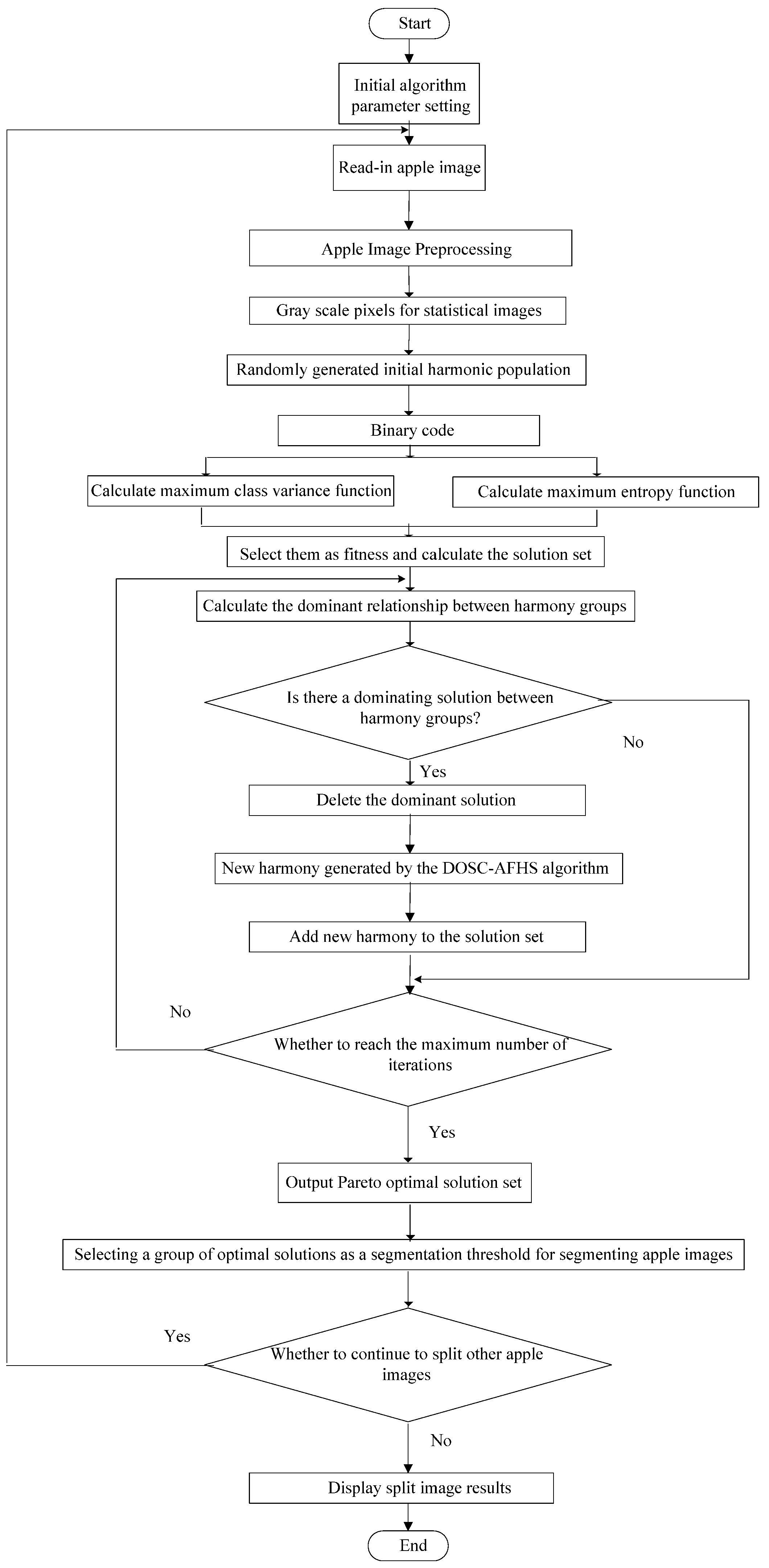
Step 1: Read and preprocess the apple image. Count the gray level of the image and the number of corresponding pixels to calculate the probability of the occurrence of grayscale.
Step 2: Enter the maximum number of evolutions , the size of the harmony memory bank HMS, and the number of tone components N.
Step 2.1: HMS initial harmony thresholds are generated randomly, which is denoted as . Each harmonic threshold is binary coded and calculated and according to Equation (9) to initialize the harmony memory. The fitness of the harmonic threshold is and .
Step 2.2: Construct a Pareto optimal solution set, and note the harmonic threshold deleted from the optimal solution set as .
Step 2.3: Each tone component of the harmony threshold is updated according to the SC-AHS algorithm step.
Step 2.4: Determine whether the number of evolutions has been reached . If not, go to Step 2.2. Otherwise, the algorithm stops and the optimal harmonic threshold solution set is output and noted as .
Step 3: Use the optimal harmony threshold solution set to divide the apple image and output the segmented image.
The apple image recognition multi-objective method based on an adaptive harmony search algorithm with simulation and creation process is shown in Figure 1.
5. Experiment Design and Results Analysis
5.1. Experiment Design
The experimental samples were chosen from the mature HuaNiu apples. A series of mature HuaNiu apple image segmentation experiments are conducted under six conditions of direct sunlight with strong, medium, and weak illumination, and backlighting with strong, medium, and weak illumination in a natural scene. The experiment contains two parts. Firstly, the benchmark functions are used to test the optimization performance of the SC-AHS algorithm. Secondly, the ARMM-AHS method is used to segment and identify the apple image. The experiment used a Lenovon (Beijing, China) Notebook computer with an Intel Core i5 CPU 2.6 GHz and 4.0 GB of memory. The test platform was Microsoft Visual C++ 6.0 and Matlab 2012.
5.2. Benchmark Function Comparison Experiment and Result Analysis
Five benchmark functions, including Sphere, Rastrigrin, Griewank, Ackley, and Rosenbrock, were used to simulate the individual fitness of harmony. The parameters of each function are shown in Table 1 [40].
5.2.1. Fixed Parameters Experiment
The fixed parameters experiment uses a minimum value optimization simulation to compare and test the optimization performance of the HS, Improved Harmony Search (IHS) [7], Global-best Harmony Search (GHS) [41], Self-adaptive Global best Harmony Search (SGHS) [24], and SC-AHS algorithms.
In the fixed parameter experiment, the experimental parameters were set as follows. HMS = 200, HMCR = 0.9, PAR = 0.3, BW = 0.01, = 20,000, N = 30. The HCMR is the Harmony memory library probability, the PAR is the tone fine-tuning probability, the BW is the tone fine-tuning bandwidth, and is the number of evolutions. In the IHS algorithm, the pitch tune probability minimum value PARmin = 0.01, the pitch tuning probability maximum value PARmax = 0.99, the pitch tune bandwidth minimum value BWmin = 0.0001, and the pitch tune bandwidth maximum value [7]. In the GHS algorithm, PARmin = 0.01, PARmax = 0.99 [41]. In the SGHS algorithm, the initial probability value of the harmony memory is HMCRm = 0.98, the standard deviation of the value of the harmony memory is HMCRs = 0.01, and the probability of the harmony memory is normally distributed within [0.9, 1.0], the average initial value of the bandwidth is PARm = 0.9, the standard deviation of the pitch tune bandwidth PARs = 0.05, the pitch tune bandwidth is normally distributed within [0.0, 1.0], the specific evolution numbers LP = 100 [24], the pitch tune bandwidth minimum BWmin = 0.0001, and the pitch tune bandwidth maximum [7]. Upper Bound (UB) is the maximum value of the search range of the algorithm, and Lower Bound (LB) is the minimum value of the search range of the algorithm. In the SC-AHS algorithm, , . The final test results were averaged after 30 independent runs. The performance evaluation of the algorithm uses the following methods: (1) the method of convergence accuracy and speed of the analysis algorithm under a fixed evolutionary frequency; and (2) the method of comparing the evolution curve of the average optimal value of each function.
The convergence accuracy of each algorithm is shown in Table 2. For both the unimodal Sphere (f1) and Rosenbrock (f5) functions, the data in Table 2 shows that the algorithm has reached the theoretical minimum of 0 for both functions. It shows that the convergence accuracy of this algorithm is very high, and the convergence speed and accuracy of other functions are slightly smaller than the SC-AHS algorithm. For the multimodal Rastrigrin (f2) function, Table 2 shows that the SC-AHS algorithm has reached the theoretical minimum of 0. It indicates that the algorithm has high convergence accuracy, and the convergence accuracy of other functions does not reach the theoretical minimum. For multimodal Griewank (f3) and Ackley (f4) functions, the data in Table 2 shows that the GHS algorithm reached the theoretical minimum value of 0 as it reaches the 5000 iterations in the Griewank (f3) function optimization. At the same time, the convergence accuracy of the GHS algorithm in the Ackley (f4) function optimization is also better than other algorithms, indicating that for these two functions, the SC-AHS algorithm converges faster, and the convergence accuracy is better than the other algorithms, except the GHS algorithm.
By comparing the minimum values of the HS, HIS [7], GHS [41], and SGHS [24] algorithms, and the SC-AHS algorithm with fixed parameters, the results show that for unimodal Sphere (f1) and Rosenbrock (f5) functions and multimodal Rastrigrin (f2) function, the SC-AHS algorithm has better performance than the other algorithms. For the multimodal Grievenk (f3) and Ackley (f4) functions, the SC-AHS algorithm converges faster than other algorithms. In addition to the GHS algorithm, the SC-AHS algorithm has better convergence accuracy than other algorithms. For each function, compared with the HS algorithm, the convergence accuracy and speed of the SC-AHS algorithm are significantly improved. Compared with other algorithms, the SC-AHS algorithm has the advantage of fast convergence.
5.2.2. Dynamic Parameters Experiment
The dynamic parameters experiment uses two test methods, including varying the number of harmony tone components and varying the harmony memory size, HMS. Under the condition of dynamic parameters, the optimization performance effect of the above algorithms, like HS, HIS [7], GHS [41], SGHS [24], and the SC-AHS is compared. The average value of each function, the relative change rate [42], and the average change value were used as measures of the performance of the algorithm.
Test of Average Optimum with Different Harmony Tone Components of Five Functions
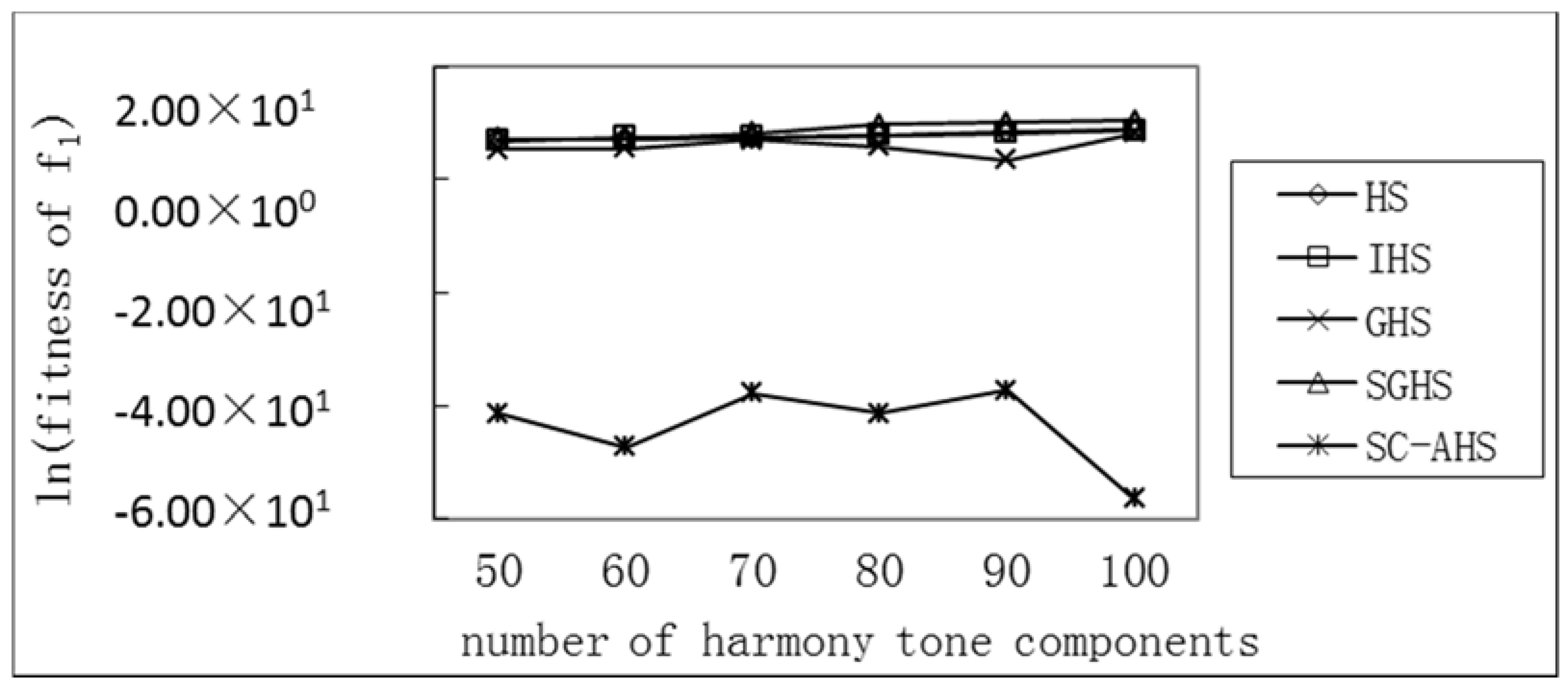
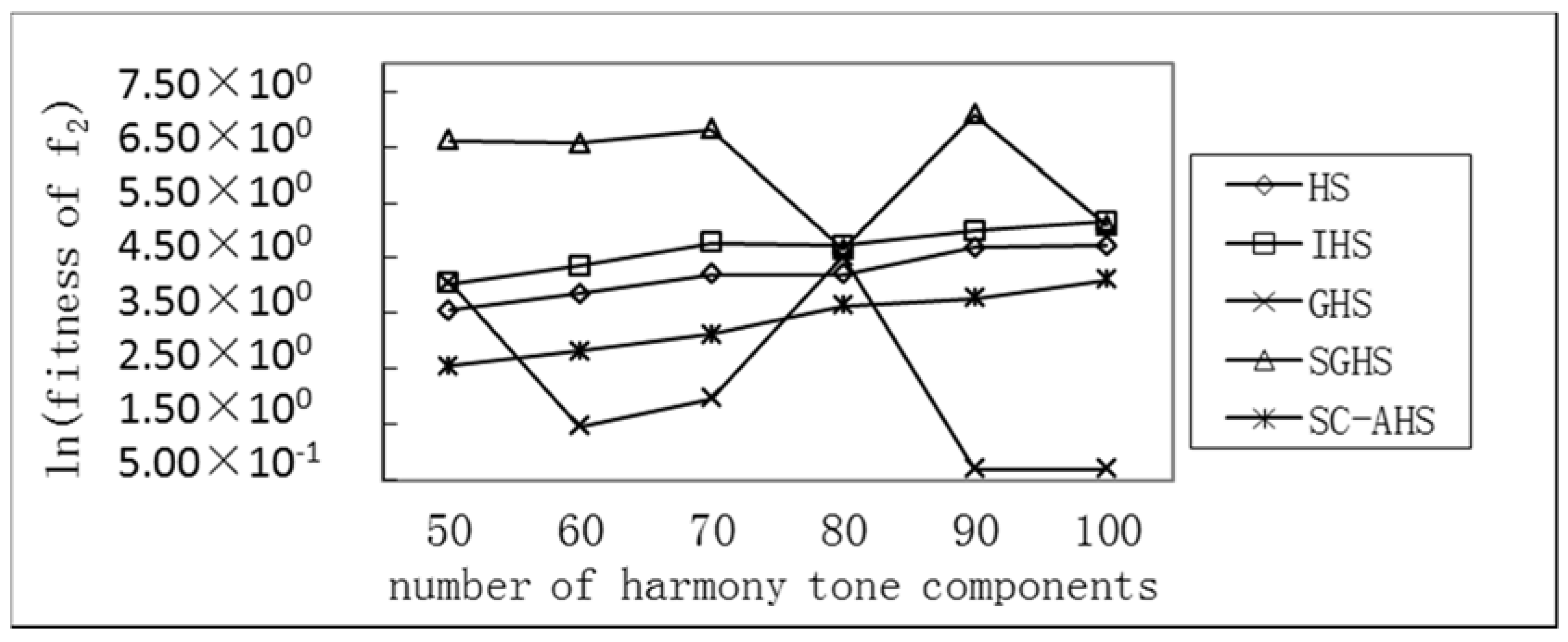
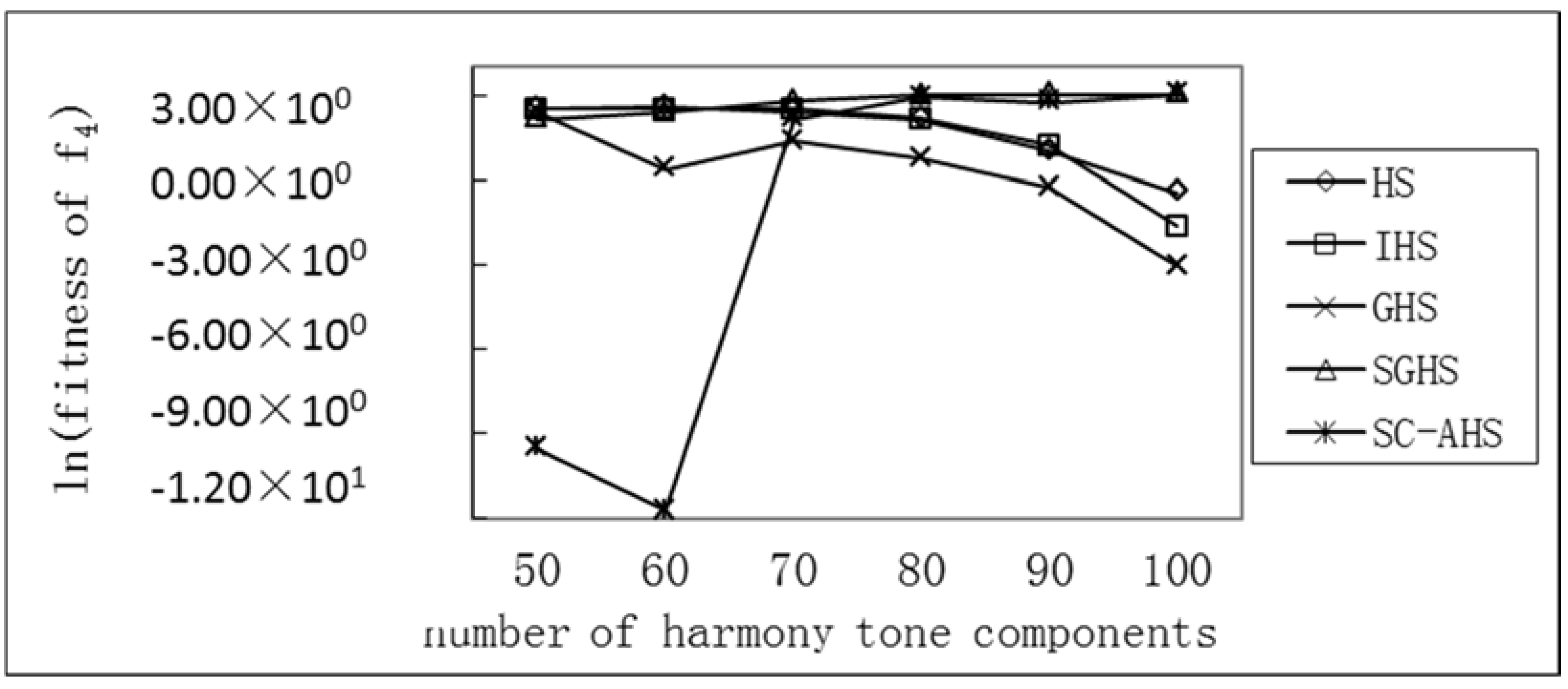
The number of harmony tone components corresponds to the dimension of the function. High-dimensional, multimodal, complex optimization problems can easily cause a local optimum and premature convergence. For this reason, it is extremely necessary to adjust the dimension of the benchmark function (i.e., the number of tone components) and test the optimization performance of each algorithm in high dimensions. The tone components are in the range of 50 to 100, and the other parameters are unchanged. The comparison of the changes in the number of tone components for the optimization performance of each algorithm is shown in Table 3. The average optimal value of each function varied with the number of tone components is shown in Figure 2, Figure 3, Figure 4, Figure 5 and Figure 6. In Table 3, there is:
It can be seen from the above that for the uni-peak Sphere (f1) and Rosenbrock (f5) functions, the average optimal value of each algorithm has an increasing trend with the increase of the number of harmonic components, but the SC-AHS algorithm shows a decline. In the trend, the relative change rate of the SC-AHS algorithm in Table 3 is also the lowest. For the multi-peak Rastrigrin (f2), Griewank (f3), and Ackley (f4) functions, the average optimal value of the SC-AHS algorithm varies unstably. The average change value of the SC-AHS algorithm in Table 3 is the lowest among the algorithms. Therefore, the SC-AHS algorithm does not show a significant decrease in convergence accuracy with the increase in the number of tone components. That is, the algorithm still has good convergence performance in high-dimensional cases.
Test of the Average Optimum with Different Harmony Memory Sizes of Five Functions
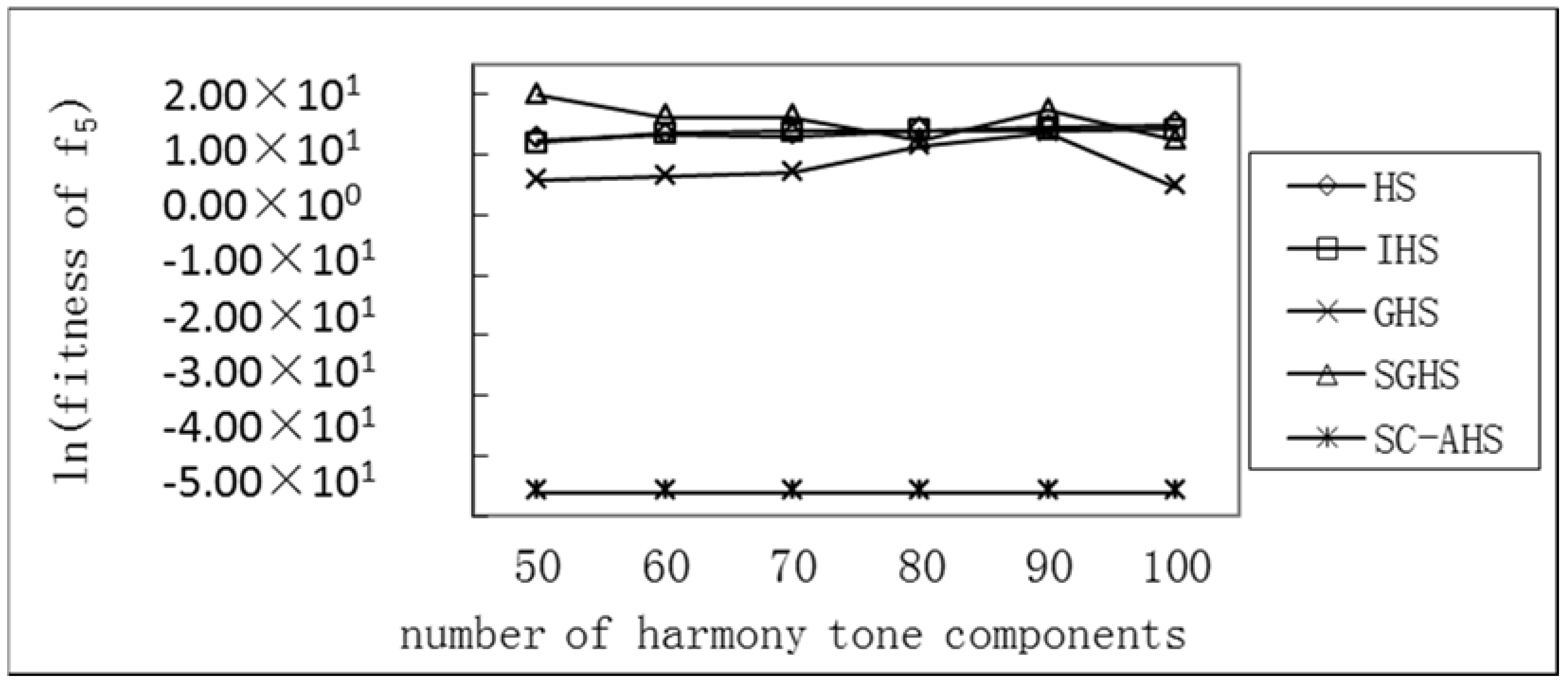
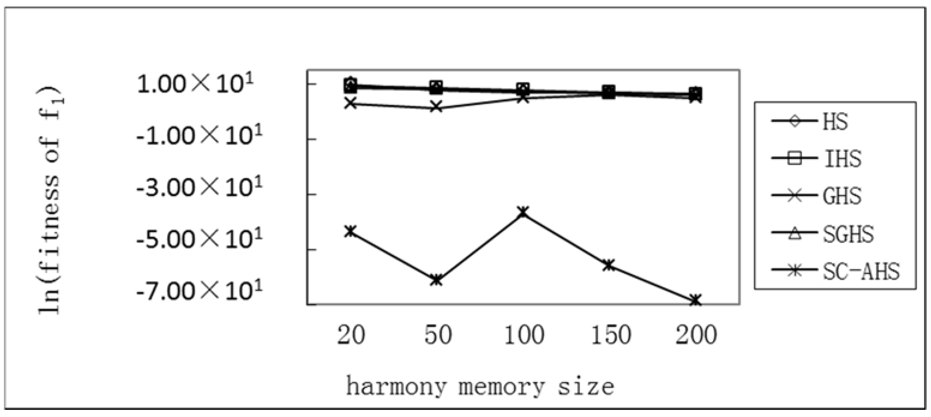
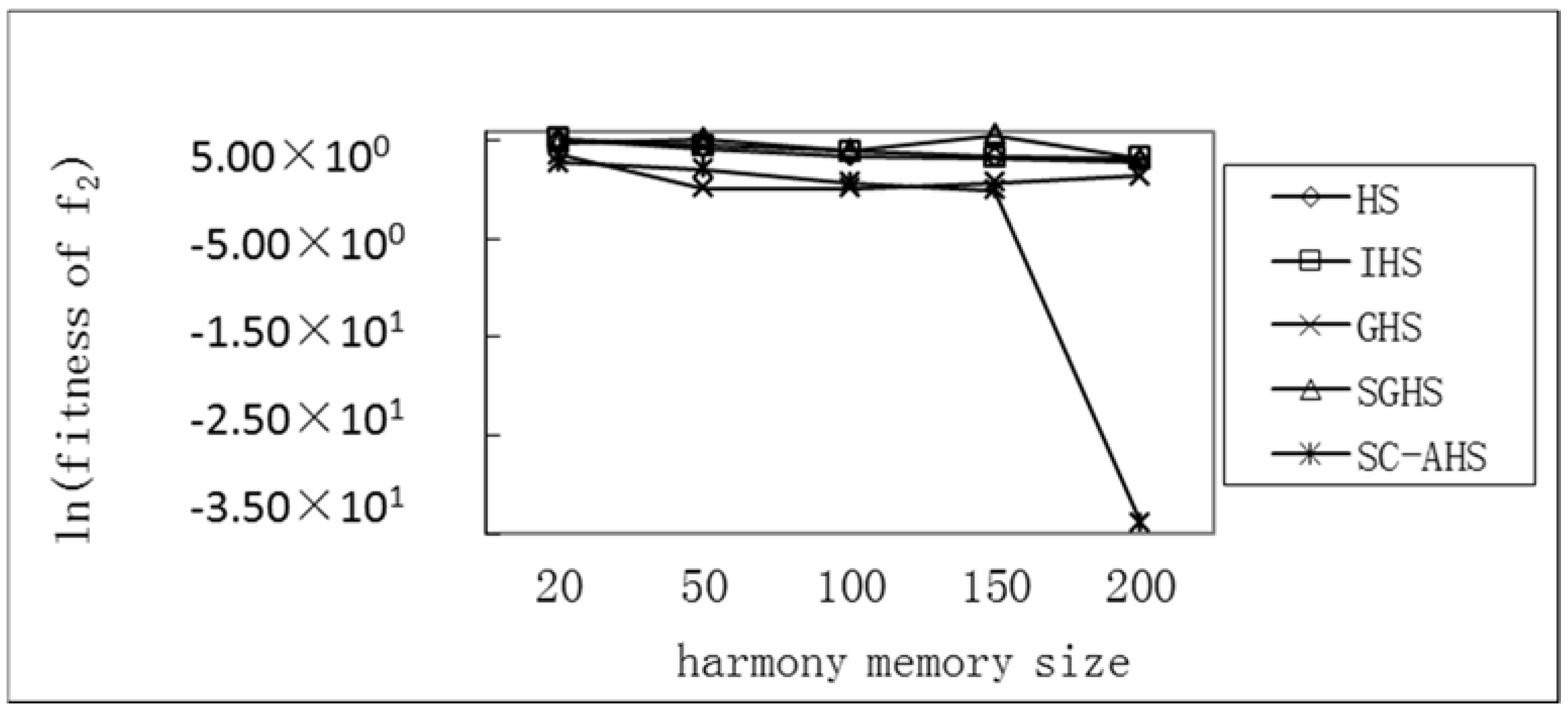
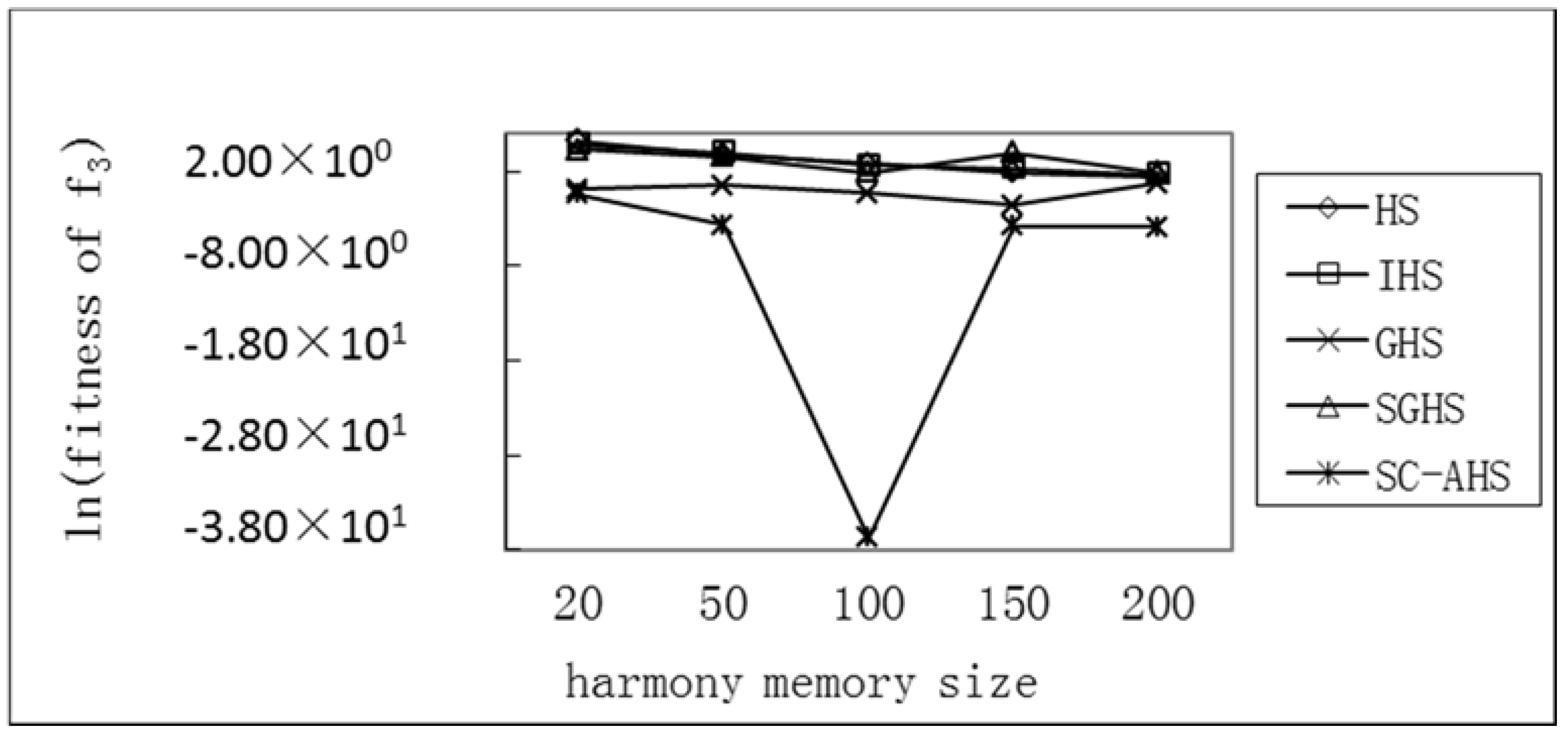
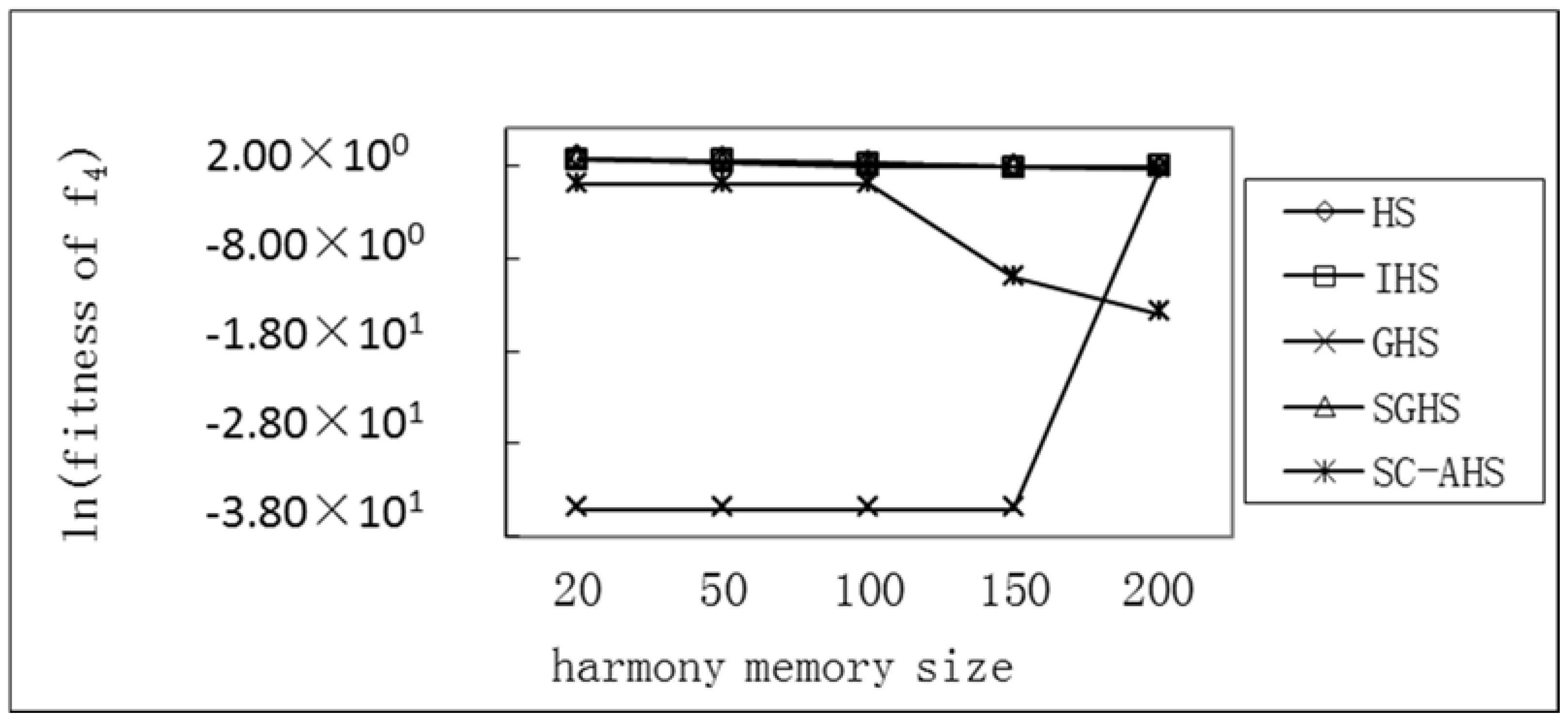
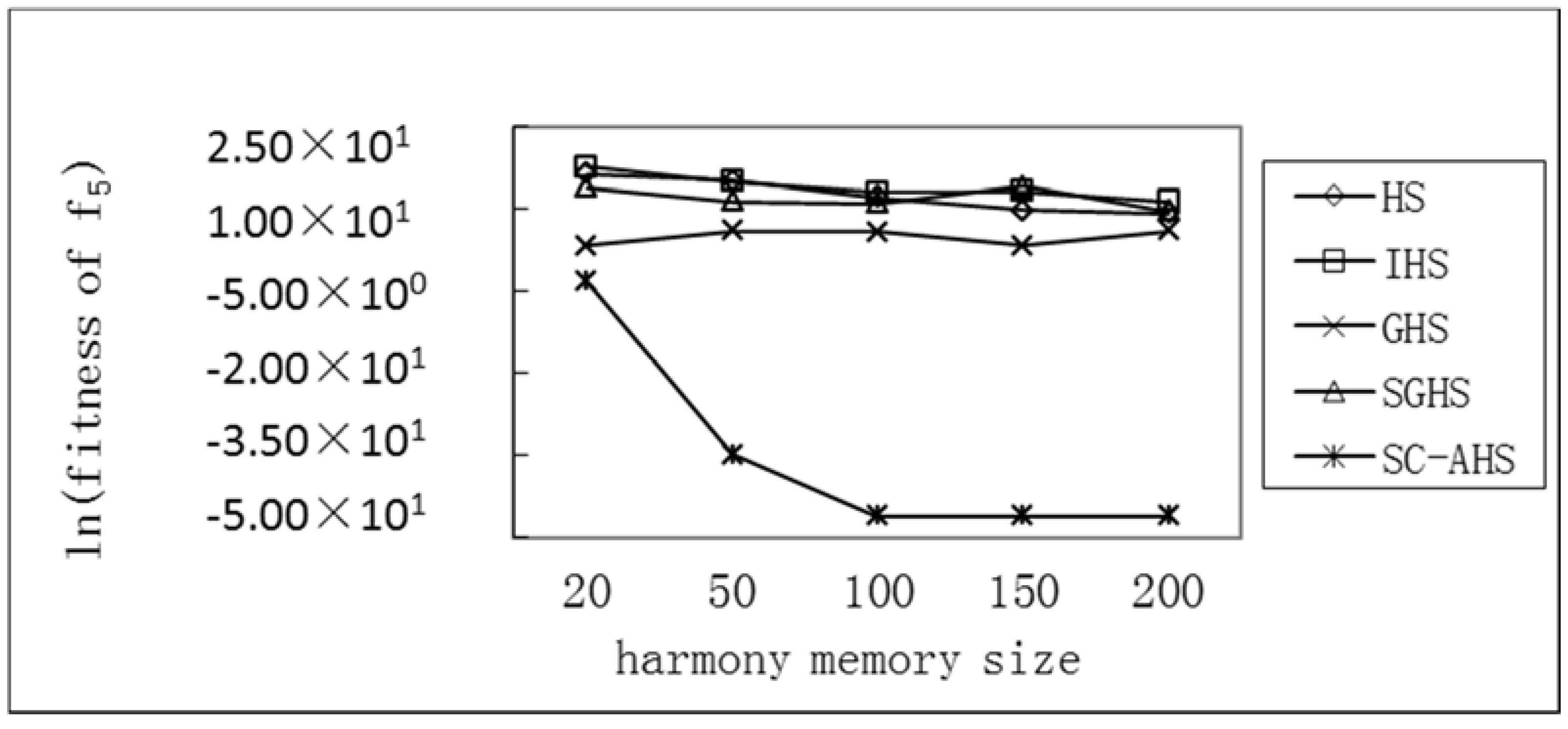
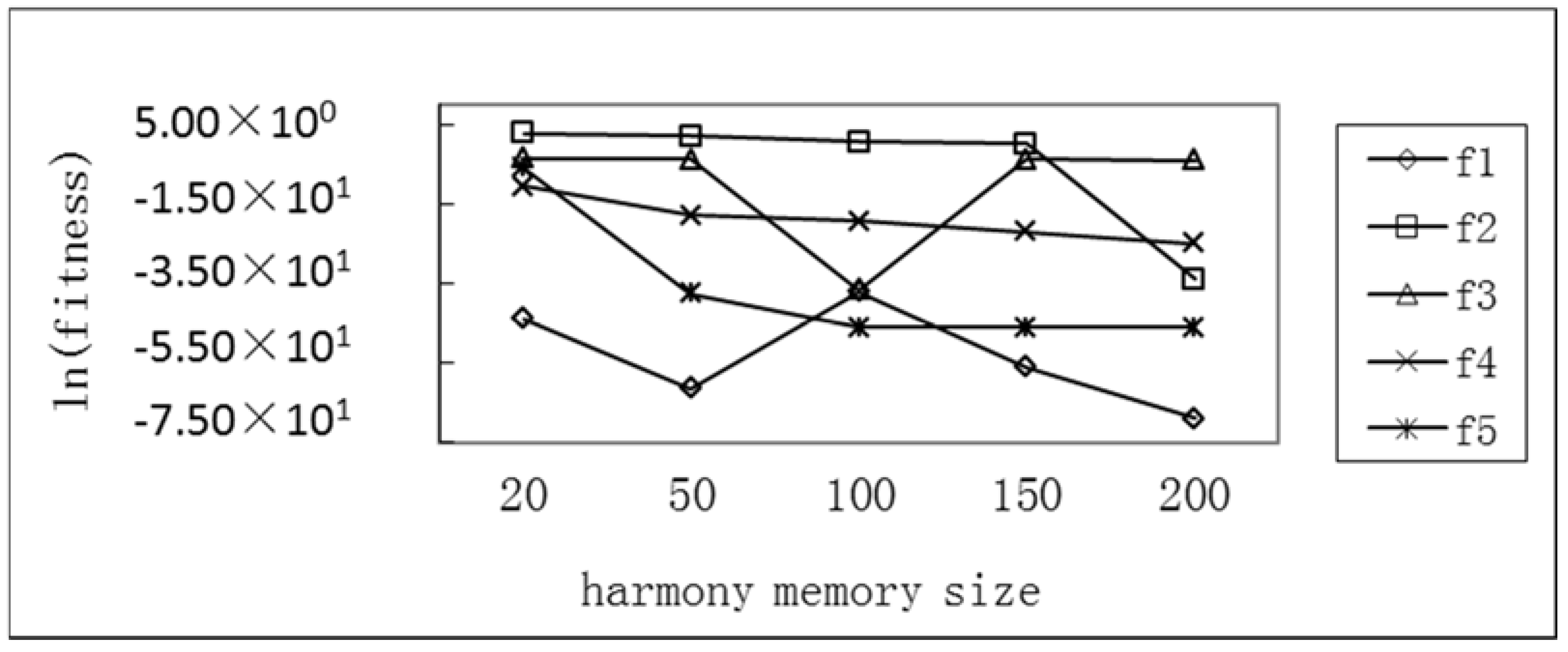
The population diversity can be affected with the changes of the size of the harmony memory HMS. The range of parameters HMS is 20, 50, 100, 150, and 200. Other parameters are unchanged. The effect of the change in the size of the harmony memory on the optimization performance of each algorithm is shown in Table 4. The comparison of the average optimum value of each function changed with the size of the harmony memory as showed in Figure 7, Figure 8, Figure 9, Figure 10 and Figure 11.
It can be seen that for the single-peak Sphere (f1) and Rosenbrock (f5) functions and the multi-peak Rastrigrin (f2) function, the average value of each algorithm has an increasing trend with the increase of the size of the harmony memory, but the SC-AHS algorithm shows a significant downward trend. The relative change rate of the SC-AHS algorithm in Table 4 is higher than other algorithms, indicating that with the increase of the size of the harmony memory, the diversity of the population is maintained and the convergence accuracy is improved. For the multi-peak Grievenk (f3) and Ackley (f4) functions, the average optimal value of the SC-AHS algorithm is not stable. The average change value of the SC-AHS algorithm in Table 4 is the lowest among the algorithms, and the relative change rate of the algorithm is higher than other algorithms. Therefore, the SC-AHS algorithm increases the convergence accuracy of the algorithm with the increase of the size of the harmonic memory, and it has better convergence than other algorithms.
5.2.3. Test of SC-AHS Algorithm with Dynamic Parameters Experiment
The experiment is mainly to verify that the SC-AHS algorithm has fast convergence performance. The experiment still adopts the conditions of changing parameters, and still adopts two test methods, including varying the number of harmonic components and varying the harmonic memory size, HMS. The effect of changing the parameters under test on the convergence speed of the SC-AHS algorithm is studied. The average optimal value of each function and the number of evolutions are used as a measure of the performance of the SC-AHS algorithm.
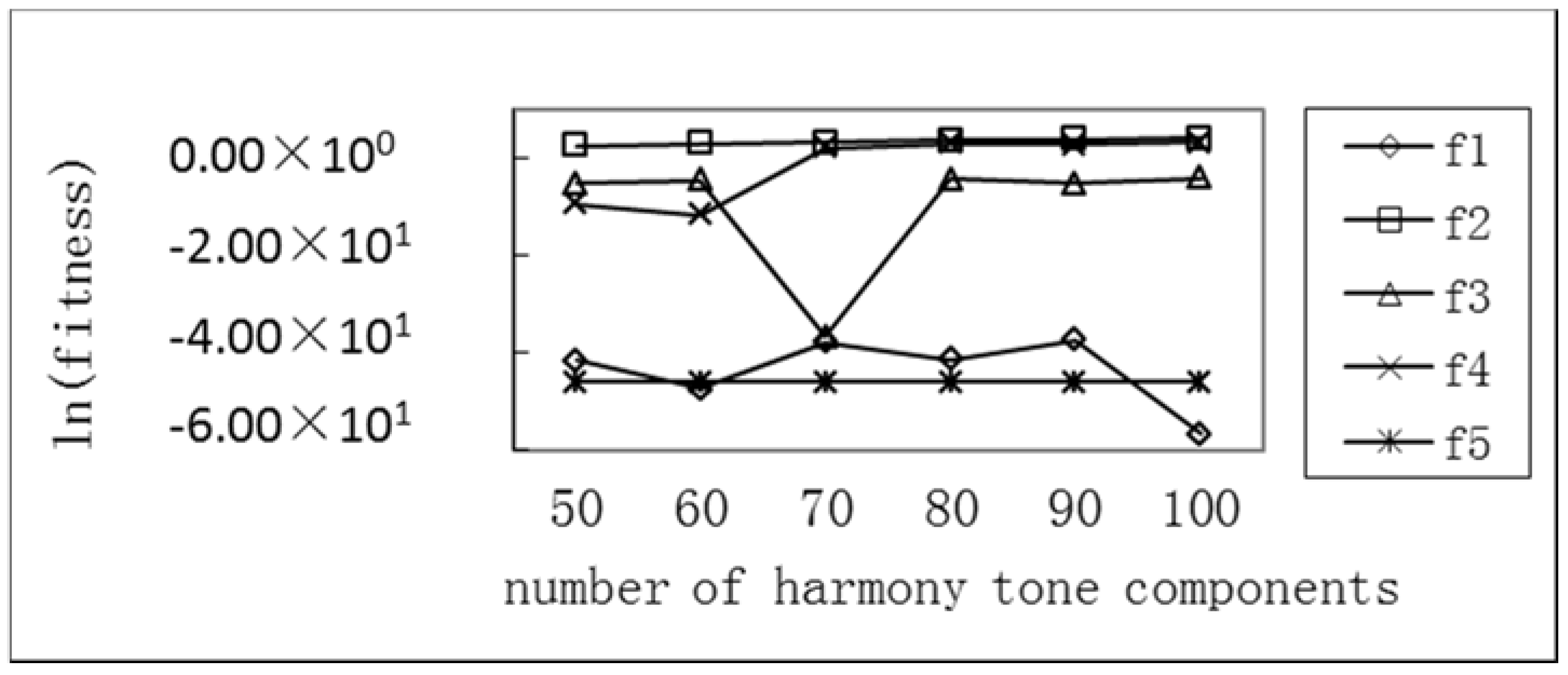
Test of Average Optimum with Different Harmony Tone Components of the SC-AHS Algorithm
The range of the number of harmonic components, N, is from 50 to 100. The other parameters are unchanged. The effect of the change in the number of harmonic components on the convergence rate of the SC-AHS algorithm is shown in Table 5. The comparison of the change of the average optimum value and the sum of the tone components of each function is shown in Figure 12. It can be seen that with the increase in the number of tone components, there is no apparent upward trend in the average optimal value of the functions. Table 5 shows that the number of evolutions of the SC-AHS algorithm is less than 20,000 for single-peak Sphere (f1) and Rosenbrock (f5) functions, as well as multi-peak Grievenk function (f3), and the number of tone components is different, indicating that the SC-AHS algorithm still has a high convergence speed in the high-dimensional case.
Test of Average Optimum with Different Harmony Memory Sizes of the SC-AHS Algorithm
The value range of the HMS memory size is also 20, 50, 100, 150, and 200, respectively, and the other parameter settings are unchanged. The effect of the change in the size of the harmony memory on the convergence rate of the SC-AHS algorithm is shown in Table 6. The comparison of the average optimum value of each function with the change of the size of the harmony memory is shown in Figure 13. It can be seen that, as the size of the harmonic memory increases, the average optimal value of each function has a more obvious downward trend. This is because the size of the harmonic memory increases, which increases the diversity of the population and the search performance of the algorithm. Table 6 shows that the number of SC-AHS evolutions is lower than 20,000 for single-peak Sphere (f1), Rosenbrock (f5), multi-peak Rastrigrin (f2), and Griewank (f3) functions. It shows that the SC-AHS algorithm has increased the convergence speed when the harmony memory is large.
5.3. Apple Image Segmentation Experiment
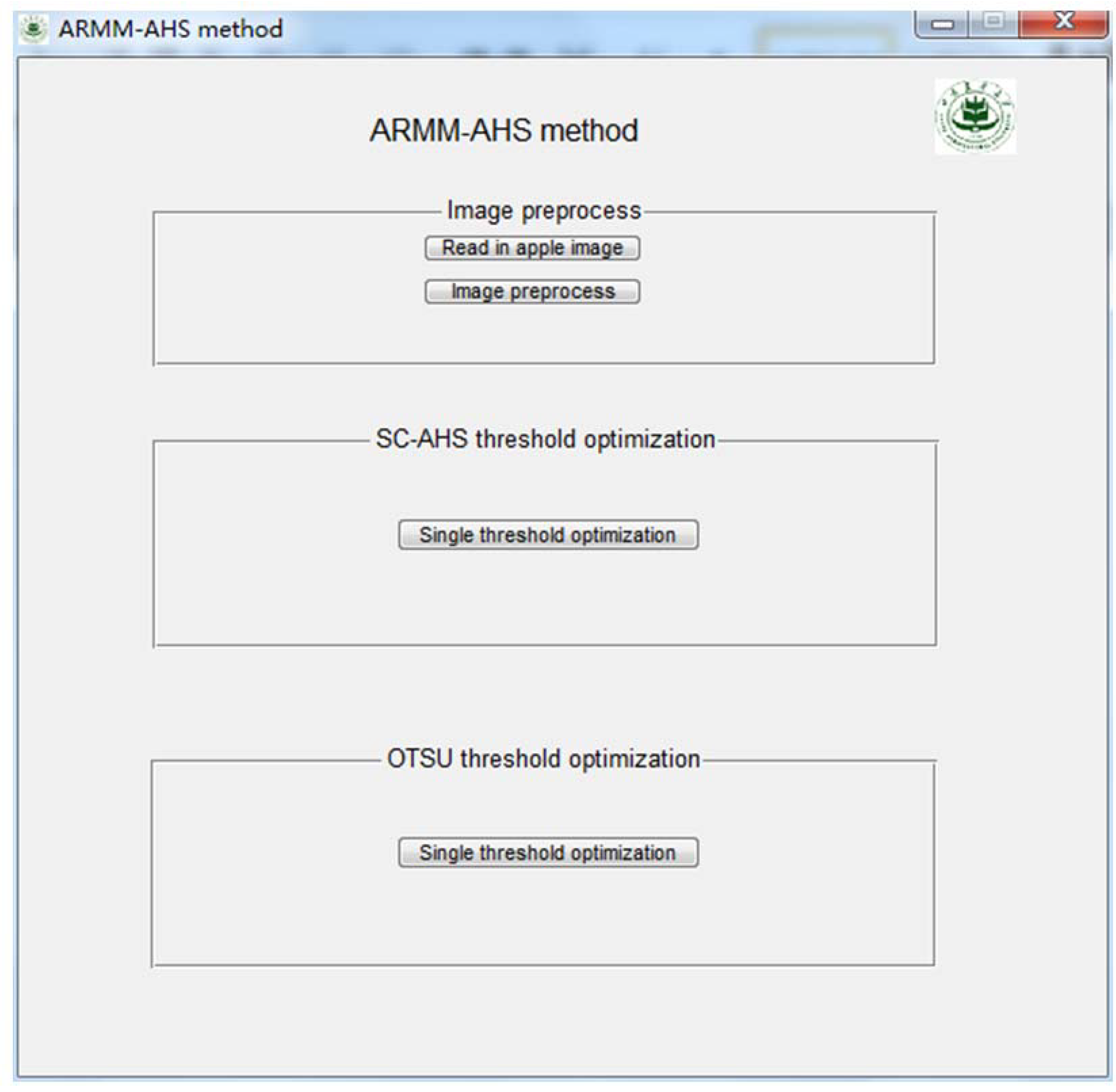
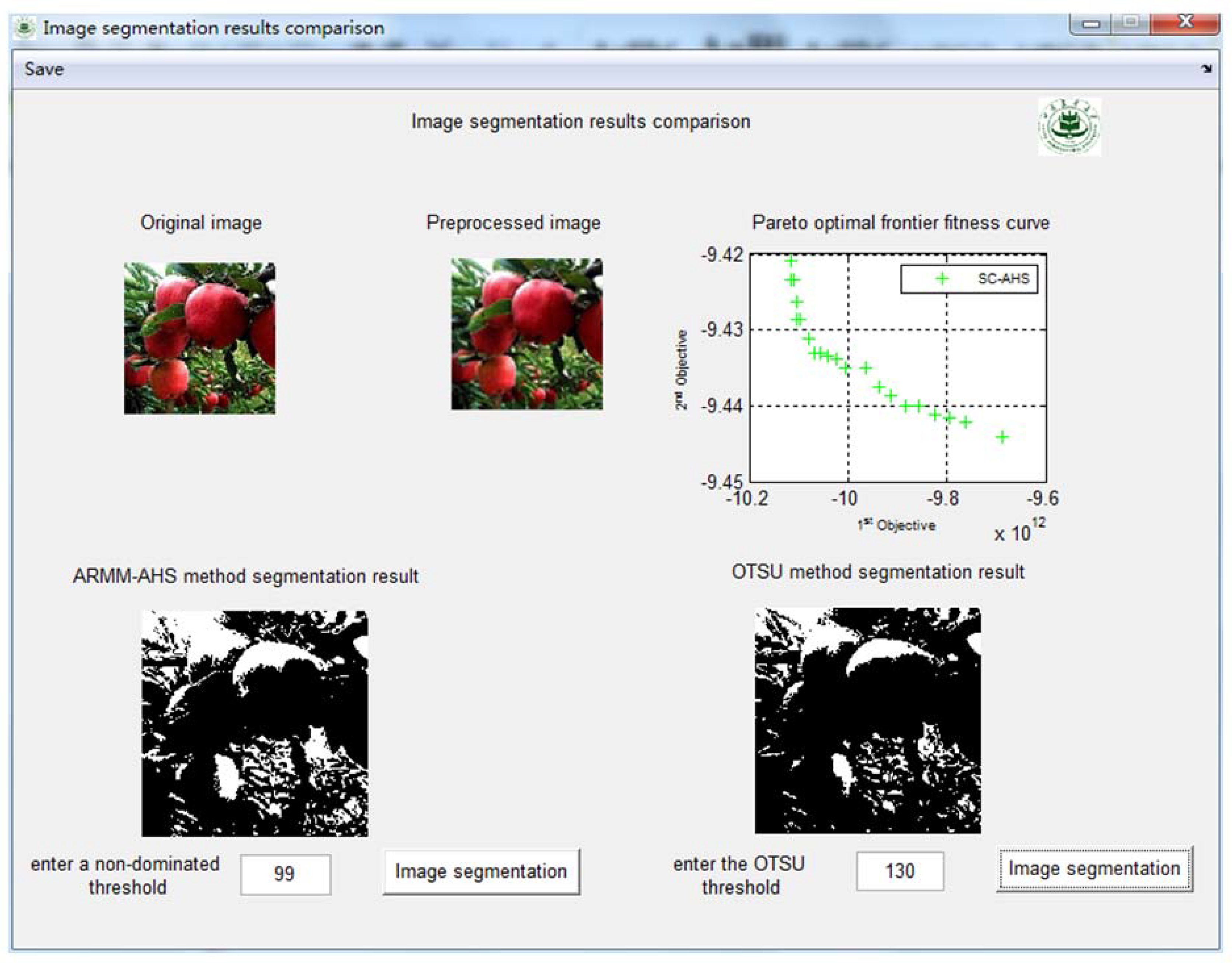
The experiment uses a single apple image as input, and takes the ARMM-AHS method proposed in this paper as the threshold search strategy of images to perform apple image segmentation experiments. The maximum class variance function and the maximum entropy function are used as the two objective fitness functions of the multi-objective optimization method. The main interface of the apple image segmentation program developed with Matlab2012 GUI is shown in Figure 14.
Five segmentation indicators based on the image recognition rate, such as the segmentation rate (RSeg), fruit segmentation rate (RApp), branch segmentation rate (RBra), segmentation success rate (RSuc), and missing rate (RMis), are respectively defined in this paper. The equations of the five indicators are defined in Equations (19)–(23). Among them, is the total number of segmentation targets (including the number of fruits and the number of branches), is the total number of targets obtained by manual visualization (including the number of fruits and the number of branches), is the total number of segmentation fruits, is the total number of fruits obtained by manual visualization, and is the total number of segmentation branches. Due to the effects of the illumination condition and interference factors, the experiment sets the fruit size that is greater than 1/4 that of complete fruit as a fruit statistics value, and sets the branch length that is greater than 1/4 that of a complete branch as a branch of the statistics value, and fruits that are too small in the perspective of the image are not counted in the statistics values.
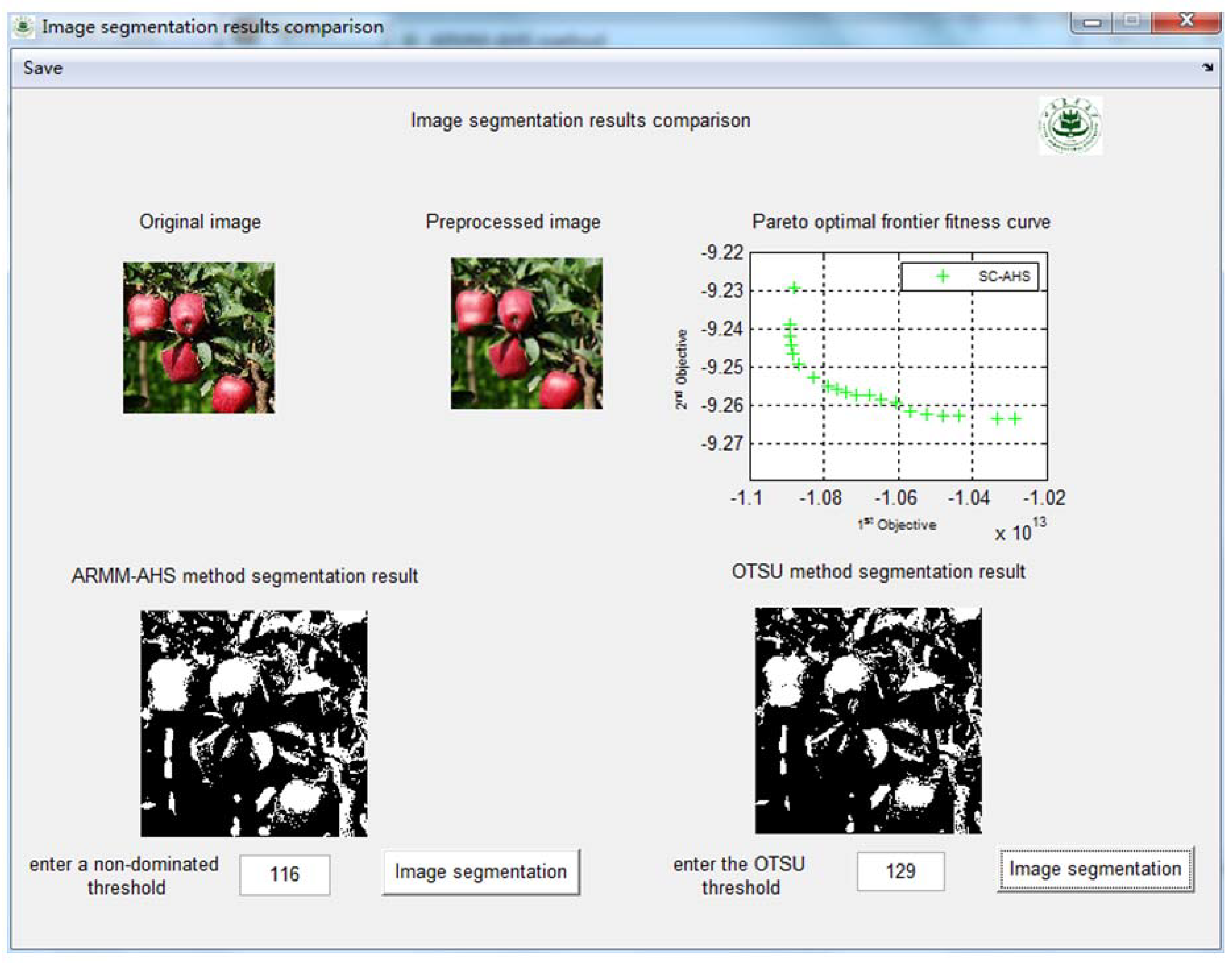
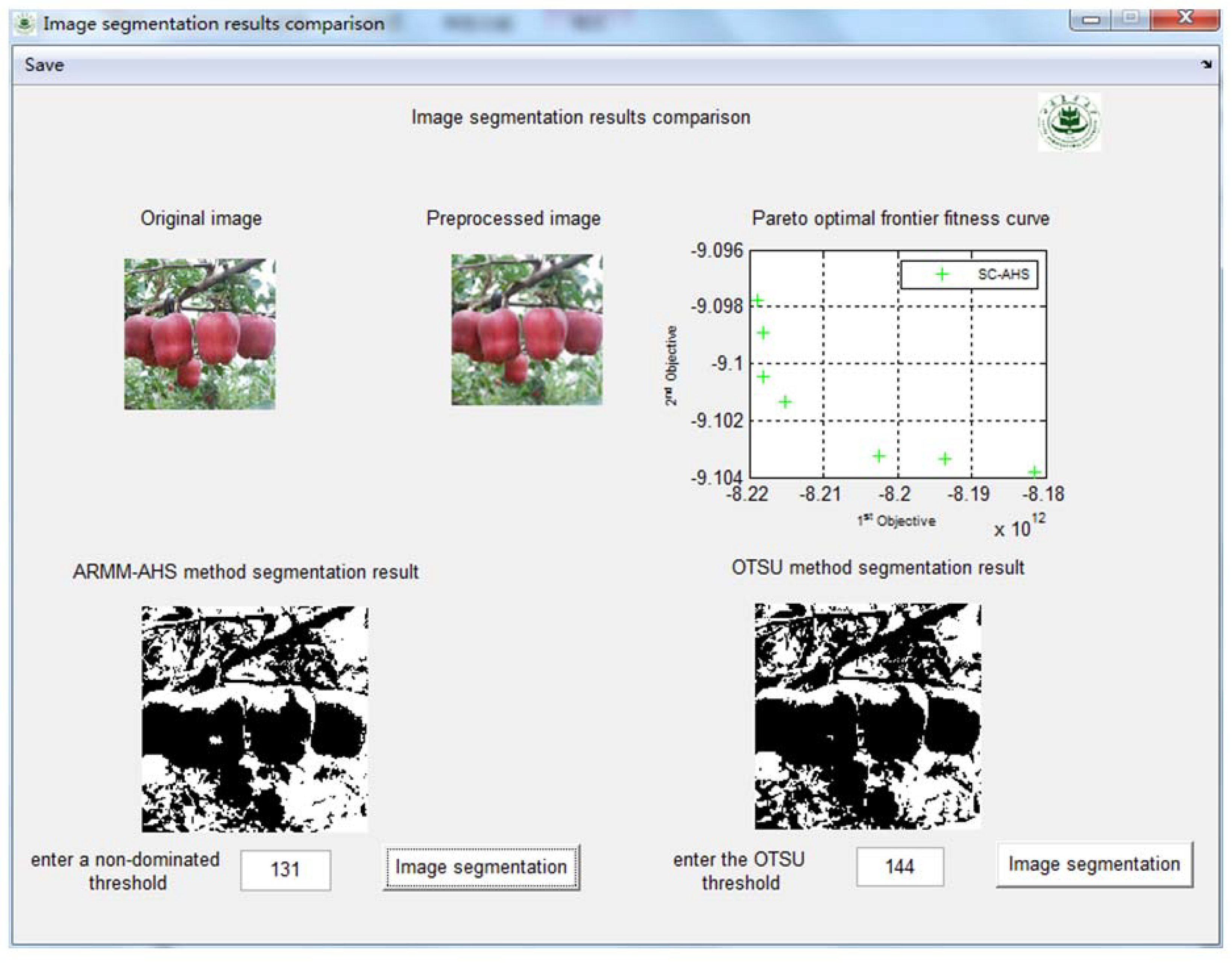
Figure 15, Figure 16 and Figure 17 show the comparison of the results of image segmentation under three illumination conditions, including direct sunlight with strong illumination, backlighting with strong illumination, and backlighting with medium illumination. The figures show the original image, the preprocessed image, the Pareto optimal frontier fitness curve using the SC-AHS optimization algorithm, the ARMM-AHS method segmentation result, and the OTSU algorithm segmentation result. Figure 15, Figure 16 and Figure 17 show that the multi-objective optimization method can be used to obtain a set of non-dominated threshold solutions, which can provide more opportunities to select thresholds. The thresholds of the non-dominated solution set under six illumination conditions using the ARMM-AHS method is shown in Table 7. The number of non-dominated solutions under six illumination conditions are different.
The comparison of the thresholds selected from the non-dominated solution set under six illumination conditions with OTSU thresholds is shown in Table 8. The effect of apple image segmentation under six lighting conditions is shown in Table 9. The data in Table 9 shows that the segmentation rate and segmentation success rate of the direct sunlight with strong illumination and backlighting with strong illumination all reach 100%. When the segmentation result includes branches, the branch segmentation rate and the missing rate are equivalent. This shows that the branches are well segmented and achieve the desired segmentation effect.
6. Conclusions
This paper proposes a new adaptive harmony search algorithm with simulation and creation, which expands the search space to maintain the diversity of the solution and accelerates the convergence of the algorithm compared with HS, HIS, GHS, and SGHS algorithms. An apple image recognition multi-objective method based on the adaptive harmony search algorithm with simulation and creation is proposed. The multi-objective optimization recognition method transforms the apple image recognition problem collected in the natural scene into a multi-objective optimization problem, and uses the new adaptive harmony search algorithm with simulation and creation as the image threshold search strategy. The proposed multi-objective optimization recognition method obtains a set of non-dominated threshold solution sets, which is more flexible than the OTSU algorithm in the opportunity of threshold selection. The selected threshold has better adaptive characteristics and has good image segmentation results.
Author Contributions
L.L. conceived and designed the multi-objective method and the experiments, and wrote the paper; J.H. performed the experiments and analyzed the experiments. Both authors have read and approved the final manuscript.
Funding
This work is supported by the National Nature Science Foundation of China (grant No. 61741201, 61462058).
Conflicts of Interest
The authors declare no conflict of interest.
References
- Zong, W.G.; Kim, J.H.; Loganathan, G.V. A new heuristic optimization algorithm: Harmony search. Simulation 2001, 76, 60–68. [Google Scholar] [CrossRef]
- Ouyang, H.B.; Xia, H.G.; Wang, Q.; Ma, G. Discrete global harmony search algorithm for 0–1 knapsack problems. J. Guangzhou Univ. (Nat. Sci. Ed.) 2018, 17, 64–70. [Google Scholar]
- Xie, L.Z.; Chen, Y.J.; Kang, L.; Zhang, Q.; Liang, X.J. Design of MIMO radar orthogonal polyphone code based on genetic harmony algorithm. Electron. Opt. Control. 2018, 1, 1–7. [Google Scholar]
- Zhu, F.; Liu, J.S.; Xie, L.L. Local Search Technique Fusion of Harmony Search Algorithm. Comput. Eng. Des. 2017, 38, 1541–1546. [Google Scholar]
- Wu, C.L.; Huang, S.; Wang, Y.; Ji, Z.C. Improved Harmony Search Algorithm in Application of Vulcanization Workshop Scheduling. J. Syst. Simul. 2017, 29, 630–638. [Google Scholar]
- Peng, H.; Wang, Z.X. An Improved Adaptive Parameters Harmony Search Algorithm. Microelectron. Comput. 2016, 33, 38–41. [Google Scholar]
- Mahdavi, M.; Fesanghary, M.; Damangir, E. An improved harmony search algorithm for solving optimization problems. Appl. Math. Comput. 2007, 188, 1567–1579. [Google Scholar] [CrossRef]
- Han, H.Y.; Pan, Q.K.; Liang, J. Application of improved harmony search algorithm in function optimization. Comput. Eng. 2010, 36, 245–247. [Google Scholar]
- Zhang, T.; Xu, X.Q.; Ran, H.J. Multi-objective Optimal Allocation of FACTS Devices Based on Improved Differential Evolution Harmony Search Algorithm. Proc. CSEE 2018, 38, 727–734. [Google Scholar]
- LIU, L.; LIU, X.B. Improved Multi-objective Harmony Search Algorithm for Single Machine Scheduling in Sequence Dependent Setup Environment. Comput. Eng. Appl. 2013, 49, 25–29. [Google Scholar]
- Hosen, M.A.; Khosravi, A.; Nahavandi, S.; Creighton, D. Improving the quality of prediction intervals through optimal aggregation. IEEE Trans. Ind. Electron. 2015, 62, 4420–4429. [Google Scholar] [CrossRef]
- Precup, R.E.; David, R.C.; Petriu, E.M. Grey wolf optimizer algorithm-based tuning of fuzzy control systems with reduced parametric sensitivity. IEEE Trans. Ind. Electron. 2017, 64, 527–534. [Google Scholar] [CrossRef]
- Saadat, J.; Moallem, P.; Koofigar, H. Training echo state neural network using harmony search algorithm. Int. J. Artif. Intell. 2017, 15, 163–179. [Google Scholar]
- Vrkalovic, S.; Teban, T.A.; Borlea, L.D. Stable Takagi-Sugeno fuzzy control designed by optimization. Int. J. Artif. Intell. 2017, 15, 17–29. [Google Scholar]
- Fourie, J.; Mills, S.; Green, R. Harmony filter: A robust visual tracking system using the improved harmony search algorithm. Image Vis. Comput. 2010, 28, 1702–1716. [Google Scholar] [CrossRef]
- Alia, O.M.; Mandava, R.; Aziz, M.E. A hybrid harmony search algorithm for MRI brain segmentation. Evol. Intell. 2011, 4, 31–49. [Google Scholar] [CrossRef]
- Fourie, J. Robust circle detection using Harmony Search. J. Optim. 2017, 2017, 1–11. [Google Scholar] [CrossRef]
- Moon, Y.Y.; Zong, W.G.; Han, G.T. Vanishing point detection for self-driving car using harmony search algorithm. Swarm Evol. Comput. 2018, 41, 111–119. [Google Scholar] [CrossRef]
- Zong, W.G. Novel Derivative of Harmony Search Algorithm for Discrete Design Variables. Appl. Math. Comput. 2008, 199, 223–230. [Google Scholar]
- Das, S.; Mukhopadhyay, A.; Roy, A.; Abraham, A.; Panigrahi, B.K. Exploratory Power of the Harmony Search Algorithm: Analysis and Improvements for Global Numerical Optimization. IEEE Trans. Syst. Man Cybern. 2011, 41, 89–106. [Google Scholar] [CrossRef] [PubMed]
- Saka, M.P.; Hasançebi, O.; Zong, W.G. Metaheuristics in Structural Optimization and Discussions on Harmony Search Algorithm. Swarm Evol. Comput. 2016, 28, 88–97. [Google Scholar] [CrossRef]
- Hasançebi, O.; Erdal, F.; Saka, M.P. Adaptive Harmony Search Method for Structural Optimization. J. Struct. Eng. 2010, 136, 419–431. [Google Scholar] [CrossRef]
- Zong, W.G.; Sim, K.B. Parameter-Setting-Free Harmony Search Algorithm. Appl. Math. Comput. 2010, 217, 3881–3889. [Google Scholar]
- Pan, Q.K.; Suganthan, P.N.; Tasgetiren, M.F.; Liang, J.J. A self-adaptive global best harmony search algorithm for continuous optimization problems. Appl. Math. Comput. 2010, 216, 830–848. [Google Scholar] [CrossRef]
- Bao, X.M.; Wang, Y.M. Apple image segmentation based on the minimum error Bayes decision. Trans. Chin. Soc. Agric. Eng. 2006, 22, 122–124. [Google Scholar]
- Qian, J.P.; Yang, X.T.; Wu, X.M.; Chen, M.X.; Wu, B.G. Mature apple recognition based on hybrid color space in natural scene. Trans. Chin. Soc. Agric. Eng. 2012, 28, 137–142. [Google Scholar]
- Lu, B.B.; Jia, Z.H.; He, D. Remote-Sensing Image Segmentation Method based on Improved OTSU and Shuffled Frog-Leaping Algorithm. Comput. Appl. Softw. 2011, 28, 77–79. [Google Scholar]
- Otsu, N. A Threshold Selection Method from Gray-Level Histograms. IEEE Trans. Syst. Man Cybern. 1979, 9, 62–66. [Google Scholar] [CrossRef]
- Kapur, J.N.; Sahoo, P.K.; Wong, A.K.C. A new method for gray-level picture thresholding using the entropy of the histogram. Comput. Vis. Graph. Image Process. 1985, 29, 273–285. [Google Scholar] [CrossRef]
- Zhao, F.; Zheng, Y.; Liu, H.Q.; Wang, J. Multi-population cooperation-based multi-objective evolutionary algorithm for adaptive thresholding image segmentation. Appl. Res. Comput. 2018, 35, 1858–1862. [Google Scholar]
- Li, M.; Cao, X.L.; Hu, W.J. Optimal multi-objective clustering routing protocol based on harmony search algorithm for wireless sensor networks. Chin. J. Sci. Instrum. 2014, 35, 162–168. [Google Scholar]
- Dong, J.S.; Wang, W.Z.; Liu, W.W. Urban One-way traffic optimization based on multi-objective harmony search approach. J. Univ. Shanghai Sci. Technol. 2014, 36, 141–146. [Google Scholar]
- Li, Z.; Zhang, Y.; Bao, Y.K.; Guo, C.X.; Wang, W.; Xie, Y.Z. Multi-objective distribution network reconfiguration based on system homogeneity. Power Syst. Prot. Control. 2016, 44, 69–75. [Google Scholar]
- Zong, W.G. Multiobjective Optimization of Time-Cost Trade-Off Using Harmony Search. J. Constr. Eng. Manag. 2010, 136, 711–716. [Google Scholar]
- Fesanghary, M.; Asadi, S.; Zong, W.G. Design of low-emission and energy-efficient residential buildings using a multi-objective optimization algorithm. Build. Environ. 2012, 49, 245–250. [Google Scholar] [CrossRef]
- Zong, W.G. Multiobjective optimization of water distribution networks using fuzzy theory and harmony search. Water 2015, 7, 3613–3625. [Google Scholar]
- Shi, X.D.; Gao, Y.L. Improved Bird Swarm Optimization Algorithm. J. Chongqing Univ. Technol. (Nat. Sci.) 2018, 4, 177–185. [Google Scholar]
- Wang, L.G.; Gong, Y.X. A Fast Shuffled Frog Leaping Algorithm. In Proceedings of the 9th International Conference on Natural Computation (ICNC 2013), Shenyang, China, 23–25 July 2013; pp. 369–373. [Google Scholar]
- Wolpert, D.H.; Macready, W.G. No free lunch theorems for optimization. IEEE Trans. Evol. Comput. 1997, 1, 67–82. [Google Scholar] [CrossRef] [Green Version]
- Wang, L. Intelligent Optimization Algorithms and Applications; Tsinghua University Press: Beijing, China, 2004; pp. 2–6. ISBN 9787302044994. [Google Scholar]
- Omran, M.G.H.; Mahdavi, M. Global-best harmony search. Appl. Math. Comput. 2008, 198, 634–656. [Google Scholar] [CrossRef]
- Han, J.Y.; Liu, C.Z.; Wang, L.G. Dynamic Double Subgroups Cooperative Fruit Fly Optimization Algorithm. Parttern Recognit. Artif. Intell. 2013, 26, 1057–1067. [Google Scholar]
Figure 1.
Flowchart of the apple image recognition multi-objective method based on an adaptive harmony search algorithm with simulation and creation.
Figure 1.
Flowchart of the apple image recognition multi-objective method based on an adaptive harmony search algorithm with simulation and creation.

Figure 2.
Comparison of the average optimum with different harmony tone components of the Sphere function.
Figure 2.
Comparison of the average optimum with different harmony tone components of the Sphere function.

Figure 3.
Comparison of the average optimum with different harmony tone components of the Rastrigrin function.
Figure 3.
Comparison of the average optimum with different harmony tone components of the Rastrigrin function.

Figure 4.
Comparison of the average optimum with different harmony tone components of the Griewank function.
Figure 4.
Comparison of the average optimum with different harmony tone components of the Griewank function.

Figure 5.
Comparison of the average optimum with different harmony tone components of the Ackley function.
Figure 5.
Comparison of the average optimum with different harmony tone components of the Ackley function.

Figure 6.
Comparison of the average optimum with different harmony tone components of the Rosenbrock function.
Figure 6.
Comparison of the average optimum with different harmony tone components of the Rosenbrock function.

Figure 7.
Comparison of the average optimum with different harmony memory sizes of the Sphere function.
Figure 7.
Comparison of the average optimum with different harmony memory sizes of the Sphere function.

Figure 8.
Comparison of the average optimum with different harmony memory sizes of the Rastrigrin function.
Figure 8.
Comparison of the average optimum with different harmony memory sizes of the Rastrigrin function.

Figure 9.
Comparison of the average optimum with different harmony memory sizes of the Griewank function.
Figure 9.
Comparison of the average optimum with different harmony memory sizes of the Griewank function.

Figure 10.
Comparison of the average optimum with different harmony memory sizes of the Ackley function.
Figure 10.
Comparison of the average optimum with different harmony memory sizes of the Ackley function.

Figure 11.
Comparison of the average optimum with different harmony memory sizes of the Rosenbrock function.
Figure 11.
Comparison of the average optimum with different harmony memory sizes of the Rosenbrock function.

Figure 12.
Comparison of the average optimum with different harmony tone components of five functions.
Figure 12.
Comparison of the average optimum with different harmony tone components of five functions.

Figure 13.
Comparison of the average optimum with different harmony memory sizes of five functions.

Figure 14.
Main interface of the apple image segmentation program.

Figure 15.
Comparison of the results of image segmentation under direct sunlight under the strong illumination condition.
Figure 15.
Comparison of the results of image segmentation under direct sunlight under the strong illumination condition.

Figure 16.
Comparison of the results of image segmentation under backlighting under the strong illumination condition.
Figure 16.
Comparison of the results of image segmentation under backlighting under the strong illumination condition.

Figure 17.
Comparison of the results of image segmentation under backlighting under the medium illumination condition.
Figure 17.
Comparison of the results of image segmentation under backlighting under the medium illumination condition.


Table 1.
Parameters of five benchmark functions.
| Function | Name | Peak Value | Dimension | Search Cope | Theoretical Optimal Value | Target Accuracy |
|---|---|---|---|---|---|---|
| f1 | Sphere | unimodal | 30 | [−100,100] | 0 | 10−15 |
| f2 | Rastrigrin | multimodal | 30 | [−5.12,5.12] | 0 | 10−2 |
| f3 | Griewank | multimodal | 30 | [−600,600] | 0 | 10−2 |
| f4 | Ackley | multimodal | 30 | [−32,32] | 0 | 10−6 |
| f5 | Rosenbrock | unimodal | 30 | [−30,30] | 0 | 10−15 |
Table 2.
Comparison of the results of fixed global evolution times.
| Algorithm | Optimization Performance | |||||
|---|---|---|---|---|---|---|
| HS | Optimum | 5.07 × 10² | 1.76 × 101 | 4.47 × 100 | 5.18 × 100 | 1.13 × 10⁴ |
| Standard deviation | 1.36 × 100 | 9.17 × 10⁻² | 4.89 × 10⁻³ | 1.88 × 10⁻² | 3.06 × 10² | |
| IHS | Optimum | 3.80 × 10² | 2.83 × 101 | 7.62 × 100 | 6.10 × 100 | 4.49 × 10⁴ |
| Standard deviation | 6.12 × 10⁻³ | 6.81 × 10⁻¹ | 8.60 × 10⁻⁶ | 1.76 × 10⁻³ | 2.26 × 101 | |
| GHS | Optimum | 1.20 × 10² | 3.62 × 10⁻⁴ | 0.00 × 100 | 5.89 × 10⁻¹⁶ | 3.00 × 101 |
| Standard deviation | 9.19 × 10⁻² | 4.70 × 10⁻² | 6.11 × 10⁻⁴ | 4.90 × 10⁻²⁹ | 3.33 × 100 | |
| SGHS | Optimum | 2.47 × 10² | 2.98 × 101 | 5.92 × 100 | 5.62 × 100 | 1.89 × 10⁴ |
| Standard deviation | 8.50 × 10⁻¹² | 1.97 × 10⁻¹ | 2.67 × 10⁻⁵ | 6.89 × 10⁻⁴ | 1.27 × 101 | |
| DOSC-AFHS | Optimum | 0.00 × 100 | 0.00 × 100 | 1.97 × 10⁻² | 3.27 × 10⁻⁶ | 0.00 × 100 |
| Standard deviation | 0.00 × 100 | 4.27 × 10⁻¹ | 1.02 × 10⁻¹⁵ | 2.72 × 10⁻⁵ | 0.00 × 100 |
Table 3.
Comparison of the optimal performance with different harmony tone components of five functions.
Table 3.
Comparison of the optimal performance with different harmony tone components of five functions.
| Functions | N | Average Optimal Value of HS | Average Optimal Value of IHS | Average Optimal Value of GHS | Average Optimal Value of SGHS | Average Optimal Value of SC-AHS |
|---|---|---|---|---|---|---|
| 50 | 1.29 × 10³ | 9.48 × 10² | 2.00 × 10² | 1.17 × 10³ | 9.62 × 10⁻¹⁹ | |
| 60 | 1.35 × 10³ | 1.96 × 10³ | 2.40 × 10² | 1.09 × 10³ | 2.49 × 10⁻²¹ | |
| 70 | 1.63 × 10³ | 1.92 × 10³ | 1.12 × 10³ | 3.59 × 10³ | 3.34 × 10⁻¹⁷ | |
| 80 | 2.67 × 10³ | 2.82 × 10³ | 3.20 × 10² | 1.82 × 10⁴ | 1.00 × 10⁻¹⁸ | |
| 90 | 4.04 × 10³ | 4.49 × 10³ | 3.20 × 101 | 2.33 × 10⁴ | 5.78 × 10⁻¹⁷ | |
| 100 | 5.83 × 10³ | 6.08 × 10³ | 3.60 × 10³ | 3.59 × 10⁴ | 2.57 × 10⁻²⁵ | |
| Relative rate of change/% | 3.52 × 10² | 5.42 × 10² | 1.70 × 10³ | 2.97 × 10³ | 1.00 × 10² | |
| Average change | 2.80 × 10³ | 3.04 × 10³ | 9.19 × 10² | 1.39 × 10⁴ | 1.55 × 10⁻¹⁷ | |
| 50 | 3.50 × 101 | 5.73 × 101 | 5.81 × 101 | 7.38 × 10² | 1.29 × 101 | |
| 60 | 4.76 × 101 | 7.81 × 101 | 4.36 × 100 | 7.09 × 10² | 1.69 × 101 | |
| 70 | 6.69 × 101 | 1.18 × 10² | 7.24 × 100 | 9.06 × 10² | 2.29 × 101 | |
| 80 | 6.75 × 101 | 1.13 × 10² | 9.30 × 101 | 1.05 × 10² | 3.78 × 101 | |
| 90 | 1.09 × 10² | 1.47 × 10² | 2.01 × 100 | 1.19 × 10³ | 4.38 × 101 | |
| 100 | 1.13 × 10² | 1.75 × 10² | 2.01 × 100 | 1.62 × 10² | 6.07 × 101 | |
| Relative rate of change/% | 2.22 × 10² | 2.06 × 10² | 9.65 × 101 | 7.80 × 101 | 3.69 × 10² | |
| Average change | 7.31 × 101 | 1.15 × 10² | 2.78 × 101 | 6.35 × 10² | 3.25 × 101 | |
| 50 | 1.03 × 101 | 8.13 × 100 | 2.80 × 100 | 1.03 × 10³ | 4.93 × 10⁻³ | |
| 60 | 1.59 × 101 | 1.66 × 101 | 1.92 × 10⁻¹ | 2.00 × 10² | 9.86 × 10⁻³ | |
| 70 | 1.77 × 101 | 1.99 × 101 | 3.52 × 100 | 1.66 × 10² | 1.11 × 10⁻¹⁶ | |
| 80 | 2.94 × 101 | 3.22 × 101 | 3.88 × 100 | 1.52 × 101 | 1.23 × 10⁻² | |
| 90 | 4.81 × 101 | 3.76 × 101 | 1.40 × 101 | 2.78 × 10² | 4.93 × 10⁻³ | |
| 100 | 4.67 × 101 | 4.96 × 101 | 3.34 × 101 | 3.52 × 101 | 1.72 × 10⁻² | |
| Relative rate of change/% | 3.56 × 10² | 5.10 × 10² | 1.09 × 10³ | 9.66 × 101 | 2.49 × 10² | |
| Average change | 2.80 × 101 | 2.73 × 101 | 9.63 × 100 | 2.88 × 10² | 8.21 × 10⁻³ | |
| 50 | 1.26 × 101 | 1.22 × 101 | 1.12 × 101 | 8.42 × 100 | 7.10 × 10⁻⁵ | |
| 60 | 1.31 × 101 | 1.25 × 101 | 1.44 × 100 | 1.07 × 101 | 7.73 × 10⁻⁶ | |
| 70 | 1.11 × 101 | 1.25 × 101 | 3.87 × 100 | 1.61 × 101 | 8.51 × 100 | |
| 80 | 8.45 × 100 | 8.93 × 100 | 2.11 × 100 | 2.00 × 101 | 1.88 × 101 | |
| 90 | 2.79 × 100 | 3.42 × 100 | 7.55 × 10⁻¹ | 2.03 × 101 | 1.56 × 101 | |
| 100 | 6.41 × 10⁻¹ | 1.96 × 10⁻¹ | 4.75 × 10⁻² | 2.05 × 101 | 2.08 × 101 | |
| Relative rate of change/% | 9.49 × 101 | 9.84 × 101 | 9.96 × 101 | 1.43 × 10² | 2.93 × 10⁷ | |
| Average change | 8.11 × 100 | 8.30 × 100 | 3.24 × 100 | 1.60 × 101 | 1.06 × 101 | |
| 50 | 2.62 × 10⁵ | 1.53 × 10⁵ | 3.03 × 10² | 4.33 × 10⁸ | 1.00 × 10⁻²⁰ | |
| 60 | 5.24 × 10⁵ | 7.42 × 10⁵ | 5.50 × 10² | 1.16 × 10⁷ | 1.00 × 10⁻²⁰ | |
| 70 | 4.95 × 10⁵ | 9.88 × 10⁵ | 1.09 × 10³ | 1.08 × 10⁷ | 1.00 × 10⁻²⁰ | |
| 80 | 1.26 × 10⁶ | 1.14 × 10⁶ | 8.46 × 10⁴ | 2.29 × 10⁵ | 1.00 × 10⁻²⁰ | |
| 90 | 2.04 × 10⁶ | 1.15 × 10⁶ | 7.97 × 10⁵ | 3.56 × 10⁷ | 1.00 × 10⁻²⁰ | |
| 100 | 3.37 × 10⁶ | 1.46 × 10⁶ | 1.00 × 10² | 2.30 × 10⁵ | 1.00 × 10⁻²⁰ | |
| Relative rate of change/% | 1.19 × 10³ | 8.55 × 10² | 6.70 × 101 | 9.99 × 101 | 0.00 × 100 | |
| Average change | 1.32 × 10⁶ | 9.39 × 10⁵ | 1.47 × 10⁵ | 8.18 × 10⁷ | 1.00 × 10⁻²⁰ |
Table 4.
Comparison of the optimal performance with different harmony memory sizes of five functions.
Table 4.
Comparison of the optimal performance with different harmony memory sizes of five functions.
| Functions | HMS | Average Optimal Value of HS | Average Optimal Value of IHS | Average Optimal Value of GHS | Average Optimal Value of SGHS | Average Optimal Value of SC-AHS |
|---|---|---|---|---|---|---|
| 20 | 2.09 × 10⁴ | 1.38 × 10⁴ | 1.60 × 101 | 4.65 × 10³ | 8.23 × 10⁻²⁰ | |
| 50 | 2.59 × 10³ | 5.33 × 10³ | 4.00 × 100 | 3.07 × 10³ | 2.14 × 10⁻²⁷ | |
| 100 | 1.02 × 10³ | 2.33 × 10³ | 1.20 × 10² | 1.68 × 10³ | 7.58 × 10⁻¹⁷ | |
| 150 | 8.41 × 10² | 1.04 × 10³ | 4.80 × 10² | 6.58 × 10² | 4.29 × 10⁻²⁵ | |
| 200 | 5.05 × 10² | 6.20 × 10² | 1.20 × 10² | 4.31 × 10² | 1.00 × 10⁻³⁰ | |
| Relative rate of change/% | 9.76 × 101 | 9.55 × 101 | 6.50 × 10² | 9.07 × 101 | 1.00 × 10² | |
| Average change | 5.16 × 10³ | 4.63 × 10³ | 1.48 × 10² | 2.10 × 10³ | 1.52 × 10⁻¹⁷ | |
| 20 | 1.60 × 10² | 1.82 × 10² | 3.49 × 101 | 1.22 × 10² | 1.59 × 101 | |
| 50 | 7.11 × 101 | 9.51 × 101 | 1.16 × 100 | 1.72 × 10² | 7.96 × 100 | |
| 100 | 3.23 × 101 | 5.28 × 101 | 1.16 × 100 | 5.40 × 101 | 1.99 × 100 | |
| 150 | 2.70 × 101 | 2.87 × 101 | 2.04 × 100 | 2.73 × 10² | 9.95 × 10⁻¹ | |
| 200 | 1.76 × 101 | 2.68 × 101 | 4.02 × 100 | 2.25 × 101 | 1.78 × 10⁻¹⁵ | |
| Relative rate of change/% | 8.91 × 101 | 8.53 × 101 | 8.85 × 101 | 8.15 × 101 | 1.00 × 10² | |
| Average change | 6.17 × 101 | 7.71 × 101 | 8.65 × 100 | 1.29 × 10² | 5.37 × 100 | |
| 20 | 1.77 × 10² | 1.25 × 10² | 1.12 × 100 | 7.10 × 101 | 6.14 × 10⁻¹ | |
| 50 | 4.32 × 101 | 5.19 × 101 | 1.60 × 100 | 3.30 × 101 | 2.46 × 10⁻² | |
| 100 | 1.70 × 101 | 1.29 × 101 | 7.20 × 10⁻¹ | 6.35 × 100 | 1.11 × 10⁻¹⁶ | |
| 150 | 6.50 × 100 | 1.01 × 101 | 1.92 × 10⁻¹ | 5.19 × 101 | 2.22 × 10⁻² | |
| 200 | 4.46 × 100 | 5.21 × 100 | 2.08 × 100 | 6.63 × 100 | 1.97 × 10⁻² | |
| Relative rate of change/% | 9.75 × 101 | 9.58 × 101 | 8.57 × 101 | 9.07 × 101 | 9.68 × 101 | |
| Average change | 4.97 × 101 | 4.11 × 101 | 1.14 × 100 | 3.38 × 101 | 1.36 × 10⁻¹ | |
| 20 | 1.54 × 101 | 1.48 × 101 | 5.89 × 10⁻¹⁶ | 1.43 × 101 | 8.97 × 10⁻¹ | |
| 50 | 1.30 × 101 | 1.24 × 101 | 5.89 × 10⁻¹⁶ | 9.69 × 100 | 8.96 × 10⁻¹ | |
| 100 | 9.06 × 100 | 9.64 × 100 | 5.89 × 10⁻¹⁶ | 5.89 × 100 | 8.96 × 10⁻¹ | |
| 150 | 6.05 × 100 | 6.22 × 100 | 5.89 × 10⁻¹⁶ | 5.89 × 100 | 4.16 × 10⁻⁵ | |
| 200 | 5.15 × 100 | 6.81 × 100 | 4.59 × 100 | 5.54 × 100 | 8.48 × 10⁻⁷ | |
| Relative rate of change/% | 6.66 × 101 | 5.41 × 101 | 7.80 × 10¹⁷ | 6.13 × 101 | 1.00 × 10² | |
| Average change | 9.73 × 100 | 9.98 × 100 | 9.19 × 10⁻¹ | 8.27 × 100 | 5.38 × 10⁻¹ | |
| 20 | 1.57 × 10⁷ | 4.96 × 10⁷ | 3.00 × 101 | 1.09 × 10⁶ | 4.36 × 10⁻² | |
| 50 | 4.17 × 10⁶ | 3.71 × 10⁶ | 4.66 × 10² | 9.13 × 10⁴ | 7.72 × 10⁻¹⁶ | |
| 100 | 2.14 × 10⁵ | 5.21 × 10⁵ | 3.76 × 10² | 7.31 × 10⁴ | 1.00 × 10⁻²⁰ | |
| 150 | 1.85 × 10⁴ | 5.58 × 10⁵ | 3.00 × 101 | 1.47 × 10⁶ | 1.00 × 10⁻²⁰ | |
| 200 | 1.08 × 10⁴ | 1.05 × 10⁵ | 4.66 × 10² | 1.67 × 10⁴ | 1.00 × 10⁻²⁰ | |
| Relative rate of change/% | 9.99 × 101 | 9.98 × 101 | 1.45 × 10³ | 9.85 × 101 | 1.00 × 10² | |
| Average change | 4.01 × 10⁶ | 1.09 × 10⁷ | 2.73 × 10² | 5.49 × 10⁵ | 8.72 × 10⁻³ |
Table 5.
Influences of convergence performance with different harmony tone components of the SC-AHS algorithm.
Table 5.
Influences of convergence performance with different harmony tone components of the SC-AHS algorithm.
| Function | Optimize Performance | N = 50 | N = 60 | N = 70 | N = 80 | N = 90 | N = 100 |
|---|---|---|---|---|---|---|---|
| Average optimal value | 9.62 × 10⁻¹⁹ | 2.49 × 10⁻²¹ | 3.34 × 10⁻¹⁷ | 1.00 × 10⁻¹⁸ | 5.78 × 10⁻¹⁷ | 2.57 × 10⁻²⁵ | |
| Evolution times/times | 309 | 414 | 480 | 548 | 620 | 765 | |
| Average optimal value | 1.29 × 101 | 1.69 × 101 | 2.29 × 101 | 3.78 × 101 | 4.38 × 101 | 6.07 × 101 | |
| Evolution times/times | 20,000 | 20,000 | 20,000 | 20,000 | 20,000 | 20,000 | |
| Average optimal value | 4.93 × 10⁻³ | 9.86 × 10⁻³ | 1.11 × 10⁻¹⁶ | 1.23 × 10⁻² | 4.93 × 10⁻³ | 1.72 × 10⁻² | |
| Evolution times/times | 20,000 | 20,000 | 19,763 | 20,000 | 20,000 | 20,000 | |
| Average optimal value | 7.10 × 10⁻⁵ | 7.73 × 10⁻⁶ | 8.51 × 100 | 1.88 × 101 | 1.56 × 101 | 2.08 × 101 | |
| Evolution times/times | 20,000 | 20,000 | 20,000 | 20,000 | 20,000 | 20,000 | |
| Average optimal value | 1.00 × 10⁻²⁰ | 1.00 × 10⁻²⁰ | 1.00 × 10⁻²⁰ | 1.00 × 10⁻²⁰ | 1.00 × 10⁻²⁰ | 1.00 × 10⁻²⁰ | |
| Evolution times/times | 5292 | 6771 | 7802 | 9855 | 10,441 | 10,890 |
Table 6.
Comparisons of the convergence performance with different harmony memory sizes of the SC-AHS algorithm.
Table 6.
Comparisons of the convergence performance with different harmony memory sizes of the SC-AHS algorithm.
| Function | Optimize Performance | HMS = 20 | HMS = 50 | HMS = 100 | HMS = 150 | HMS = 200 |
|---|---|---|---|---|---|---|
| Average optimal value | 8.23 × 10⁻²⁰ | 2.14 × 10⁻²⁷ | 7.58 × 10⁻¹⁷ | 4.29 × 10⁻²⁵ | 1.00 × 10⁻³⁰ | |
| Evolution times/times | 1606 | 280 | 203 | 219 | 209 | |
| Average optimal value | 1.59 × 101 | 7.96 × 100 | 1.99 × 100 | 9.95 × 10⁻¹ | 1.78 × 10⁻¹⁵ | |
| Evolution times/times | 20,000 | 20,000 | 20,000 | 20,000 | 18,361 | |
| Average optimal value | 3.06 × 10⁻² | 2.46 × 10⁻² | 1.11 × 10⁻¹⁶ | 2.22 × 10⁻² | 1.97 × 10⁻² | |
| Evolution times/times | 20,000 | 20,000 | 11,936 | 20,000 | 20,000 | |
| Average optimal value | 2.27 × 10⁻⁵ | 1.60 × 10⁻⁸ | 3.93 × 10⁻⁹ | 2.87 × 10⁻¹⁰ | 1.31 × 10⁻¹¹ | |
| Evolution times/times | 20,000 | 20,000 | 20,000 | 20,000 | 20,000 | |
| Average optimal value | 2.43 × 10⁻³ | 4.33 × 10⁻¹⁷ | 1.00 × 10⁻²⁰ | 1.00 × 10⁻²⁰ | 1.00 × 10⁻²⁰ | |
| Evolution times/times | 20,000 | 20,000 | 4296 | 3932 | 3346 |
Table 7.
Thresholds of the non-dominated solution set under six illumination conditions using the ARMM-AHS method.
Table 7.
Thresholds of the non-dominated solution set under six illumination conditions using the ARMM-AHS method.
| Direct Sunlight with Strong | Direct Sunlight with Medium | Direct Sunlight with Weak | Backlighting with Strong | Backlighting with Medium | Backlighting with Weak |
|---|---|---|---|---|---|
| Non-Dominated Solution Number: 54 | Non-Dominated Solution Number: 36 | Non-Dominated Solution Number: 28 | Non-Dominated Solution Number: 18 | Non-Dominated Solution Number: 54 | Non-Dominated Solution Number: 62 |
| 77 | 121 | 130 | 131 | 107 | 146 |
| 116 | 121 | 130 | 131 | 99 | 152 |
| 77 | 114 | 130 | 131 | 107 | 129 |
| 77 | 121 | 130 | 131 | 126 | 113 |
| 77 | 121 | 130 | 131 | 107 | 152 |
| 116 | 121 | 130 | 131 | 126 | 152 |
| 116 | 131 | 130 | 131 | 126 | 152 |
| 77 | 121 | 130 | 131 | 126 | 115 |
| 116 | 121 | 130 | 131 | 107 | 115 |
| 116 | 121 | 130 | 131 | 107 | 115 |
| 116 | 121 | 130 | 131 | 106 | 113 |
| 77 | 121 | 130 | 131 | 99 | 113 |
| 77 | 121 | 130 | 172 | 99 | 113 |
| 77 | 131 | 130 | 228 | 107 | 122 |
| 116 | 114 | 130 | 66 | 99 | 152 |
| 77 | 121 | 130 | 221 | 126 | 113 |
| 116 | 131 | 130 | 206 | 99 | 113 |
| 77 | 121 | 130 | 15 | 106 | 113 |
| 116 | 114 | 130 | 107 | 120 | |
| 77 | 121 | 130 | 106 | 129 | |
| 116 | 121 | 130 | 106 | 120 | |
| 77 | 121 | 46 | 99 | 129 | |
| 77 | 114 | 133 | 106 | 146 | |
| 77 | 121 | 85 | 106 | 129 | |
| 77 | 121 | 72 | 126 | 120 | |
| 77 | 121 | 146 | 107 | 120 | |
| 77 | 114 | 55 | 126 | 152 | |
| 77 | 149 | 45 | 107 | 113 | |
| 77 | 114 | 99 | 152 | ||
| 116 | 178 | 126 | 129 | ||
| 116 | 243 | 99 | 146 | ||
| 116 | 39 | 99 | 115 | ||
| 116 | 198 | 126 | 122 | ||
| 116 | 66 | 126 | 120 | ||
| 77 | 166 | 126 | 146 | ||
| 116 | 97 | 126 | 122 | ||
| 77 | 107 | 122 | |||
| 77 | 126 | 120 | |||
| 77 | 107 | 152 | |||
| 77 | 106 | 122 | |||
| 77 | 106 | 120 | |||
| 116 | 126 | 122 | |||
| 116 | 106 | 146 | |||
| 153 | 168 | 120 | |||
| 69 | 70 | 146 | |||
| 231 | 230 | 120 | |||
| 205 | 98 | 146 | |||
| 146 | 106 | 122 | |||
| 36 | 159 | 113 | |||
| 33 | 163 | 122 | |||
| 221 | 70 | 202 | |||
| 21 | 10 | 58 | |||
| 163 | 208 | 47 | |||
| 203 | 91 | 122 | |||
| 214 | |||||
| 28 | |||||
| 129 | |||||
| 209 | |||||
| 181 | |||||
| 204 | |||||
| 248 | |||||
| 172 |
Table 8.
Comparison of thresholds selected from the non-dominated solution set under six illumination conditions with OTSU thresholds.
Table 8.
Comparison of thresholds selected from the non-dominated solution set under six illumination conditions with OTSU thresholds.
| Illumination Condition | Select Threshold by SC-AHS | OTSU Threshold |
|---|---|---|
| Direct sunlight with strong | 116 | 129 |
| Direct sunlight with medium | 121 | 129 |
| Direct sunlight with weak | 130 | 133 |
| Backlighting with strong | 131 | 144 |
| Backlighting with medium | 99 | 130 |
| Backlighting with weak | 113 | 130 |
Table 9.
Apple image segmentation effect comparison under six illumination conditions.
| Illumination Condition | RSeg | RApp | RBra | RSuc | RMis (%) |
|---|---|---|---|---|---|
| Direct sunlight with strong | 100.0 | 85.7 | 14.3 | 100.0 | 0.0 |
| Direct sunlight with medium | 80.0 | 75.0 | 25.0 | 75.0 | 25.0 |
| Direct sunlight with weak | 80.0 | 100.0 | 0.0 | 80.0 | 20.0 |
| Backlighting with strong | 100.0 | 83.3 | 16.7 | 100.0 | 0.0 |
| Backlighting with medium | 85.7 | 83.3 | 16.7 | 83.3 | 16.7 |
| Backlighting with weak | 66.7 | 100.0 | 0.0 | 66.7 | 33.3 |
© 2018 by the authors. Licensee MDPI, Basel, Switzerland. This article is an open access article distributed under the terms and conditions of the Creative Commons Attribution (CC BY) license (http://creativecommons.org/licenses/by/4.0/).
Share and Cite
MDPI and ACS Style
Liu, L.; Huo, J. Apple Image Recognition Multi-Objective Method Based on the Adaptive Harmony Search Algorithm with Simulation and Creation. Information 2018, 9, 180. https://doi.org/10.3390/info9070180
AMA Style
Liu L, Huo J. Apple Image Recognition Multi-Objective Method Based on the Adaptive Harmony Search Algorithm with Simulation and Creation. Information. 2018; 9(7):180. https://doi.org/10.3390/info9070180
Chicago/Turabian StyleLiu, Liqun, and Jiuyuan Huo. 2018. "Apple Image Recognition Multi-Objective Method Based on the Adaptive Harmony Search Algorithm with Simulation and Creation" Information 9, no. 7: 180. https://doi.org/10.3390/info9070180
Note that from the first issue of 2016, this journal uses article numbers instead of page numbers. See further details here.