An Efficient Task Autonomous Planning Method for Small Satellites


School of Information Science and Engineering, Central South University, Changsha 410083, China
*
Author to whom correspondence should be addressed.
Information 2018, 9(7), 181; https://doi.org/10.3390/info9070181
Submission received: 23 June 2018
/
Revised: 15 July 2018
/
Accepted: 18 July 2018
/
Published: 20 July 2018
Abstract
:Existing on-board planning systems do not apply to small satellites with limited onboard computer capacity and on-board resources. This study aims to investigate the problem of autonomous task planning for small satellites. Based on the analysis of the problem and its constraints, a model of task autonomous planning was implemented. According to the long-cycle task planning requirements, a framework of rolling planning was proposed, including a rolling window and planning unit in the solution, and we proposed an improved genetic algorithm (IGA) for rolling planning. This algorithm categorized each individual based on the compliance of individuals with a time partial order constraint and resource constraint, and designed an appropriate crossover operator and mutation operator for each type of individual. The experimental result showed that the framework and algorithm can not only respond quickly to observation tasks, but can produce effective planning programs to ensure the successful completion of observation tasks.
1. Introduction
Task planning is an important part of satellite task control platform. Its main function is to solve the problem of resource utilization and task conflict in the task management of satellites, and to improve the service efficiency of the resources. In the traditional task planning, the ground stations calculate the task sequence in advance, based on the task requirements and satellite status estimation, and then upload it to the satellite for execution [1]. Therefore, the effectiveness of satellites cannot be fully realized in the current control mode, because the control instructions that satellites rely on are issued by the ground control system. Satellites cannot make a rapid response to the dynamic changes of the requirements due to the satellite–ground communication delay, time window, and other factors, which result in an inevitable waste of time and resources.
Small satellites are defined as being artificial satellites with low weights and a small size, which are usually under 500 kg [2]. Small satellites have several advantages, such as simple design, short development time, low cost, easy to launch, and strong survivability. The tasks that originally needed medium and large satellites can now be executed by several small satellites. For example, OneWeb plans a mega-constellation of at least 648 small satellites to provide low-delay and high-speed Internet service [3]. However, the small satellites are limited in their computing capabilities and on-board resources, because of their low cost [4]. Existing on-board planning systems usually take a long time for planning, decision making, and execution, which do not apply to small satellites with a limited onboard computer capacity. How to realize the autonomous task planning of small satellites becomes a hot topic for researchers and the related research areas that are concerned. In this paper, we use small Earth observation satellites as an object of study in this paper.
Beaumet G. [5] analyzed the feasibility of autonomous task planning of the Earth observing satellite, then proposed reaction–deliberation architecture for autonomous task planning, and designed an iterative, random greedy algorithm, but did not consider the impacts of execution on the planning. The authors of [6,7,8,9,10] deeply explored the autonomous task planning system of the Earth Observing One (EO-1) spacecraft, but the efficiency of the systems was undesirable. Chien S. [11] used the iterative repair method for autonomous task planning, but the state of the satellite changed in real-time, so it was difficult to grasp the time of the repair, and the duration of each plan could not be determined. Verfaillie G. [12] have put forward a reverse dynamic programming method, however, the planning model is relatively simple, which is quite different from the practical projects. Yanjie Song [13] established a model to solve the problem of autonomous programming for the emergency missions of agile imaging satellites, but the model has a low task completion rate when the number of general tasks is large. Other studies have analyzed the task scheduling problem from the theoretical level, developed the scheduling framework, and proposed corresponding methods, but these algorithms have shortcomings of expensive computing, which is not suitable for small satellites [14,15,16,17,18,19]. In addition, so far, most studies only consider time-dependent constraints, while few consider the resource constraints and the dynamic characteristic of resources on the satellites [20,21].
We also contrasted several articles on motion planning and task scheduling in robotics research and have had some enlightenment from them. Zacharia [22] introduced a method for simultaneously planning collision-free motion and scheduling a time-optimal route along a set of given task-points based on the improved genetic algorithm, with special encoding to encounter the multiplicity of the robot inverse kinematics. The simulation results show the efficiency and the effectiveness of the proposed approach to determining a suboptimal tour for multi-goal motion planning in complex environments cluttered with obstacles. Xidias [23] proposed a generic approach for the integration of vehicle routing and scheduling, and motion planning for a group of autonomous guided vehicles, and their method realized the time-optimum and collision-free paths for all autonomous guided vehicles. These papers give us some inspiration for the autonomous task planning of small satellites.
This paper will discuss and analyze the difficulties in the time-dependent and resource-dependent task planning of small satellites, as well as put forward the task planning model based on various constraints. On the basis of the above literature, we will propose a rolling-planning framework of on-board autonomous task planning and an improved genetic algorithm for rolling planning, in order to meet the need of real-time tasks.
The rest of the paper is organized as follows. The second part will propose the model of the task planning and specify the corresponding restriction conditions. Then, the framework and algorithms to solve this problem will be presented in the third part. In the fourth part, the feasibility and effectiveness of the proposed method will be verified by an example. Finally, the conclusion is given in the fifth part.
2. Question Description and Modeling
2.1. Problem Description
The working environment on the satellite changes dynamically over time, which is mainly reflected in two aspects, the tasks and satellite status. The change of tasks is determined by the tenant’s needs and weather conditions, for example, the user may propose a new task at any time, and some tasks may be cancelled temporarily because of cloud cover. The change of satellite state means that every task performed by the satellites will have some influence on the on-board memory, battery, and other resources, and the impact cannot be accurately predicted before the task is completed.
Therefore, the autonomous task planning problem of small satellites can be described as follows: A set of tasks need to be accomplished by small satellites, but the small satellites are limited in their computing capabilities and on-board resources. The task planning can efficiently accomplish the observation task and the data-downloading tasks without intervention of the ground. In this way, the satellite can not only respond quickly to task demands, but can also perform as many tasks as possible, providing maximum observation profits.
The difficulties are as follows:
- It is difficult to properly design the mode and framework so that real-time response and optimization of task planning can be integrated on board.
- The operation ability of small satellite is limited, and the planning algorithms need to be adapted to the resources on the satellite. For this reason, it is difficult to design an efficient algorithm.
In this article, we analyzed the previous research and proposed a model based on the following assumptions.
Assumption 1.
A single satellite has only one remote sensor.
Assumption 2.
The satellite cannot be charged during the time of umbra or penumbra, while it can be charged constantly during the rest time.
Assumption 3.
We divided tasks into common tasks and data-downloading tasks. The data-downloading tasks do not participate in the optimization.
Assumption 4.
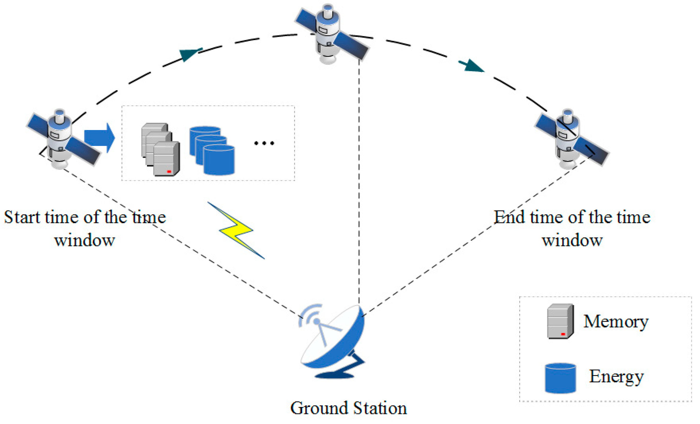
The data-downloading tasks automatically execute when the following conditions are met: (1) the satellite runs in the time window; (2) there is data in the on-board memory; and (3) electricity is available (as shown in Figure 1).
Assumption 5.
The planning system can communicate effectively with other systems on the satellite and execute the corresponding commands in a timely manner.
2.2. Model Input
represents the set of dynamic observation tasks. Each task, j, has its corresponding priority , that is, the profit of the observation task. and represent the size of memory and the maximum storage capacity that the satellite can use for planning. represents the current charge of battery and represents the maximum electricity that the satellite can use for planning. and represent the start time and end time of the i-th observation time window, respectively. C represents the charge rate of the satellite.
2.3. Model Output
and represent the decision variables in the model, ; where indicates that task is selected, indicates that task is completed. If task j is completed, that is, and , otherwise, . and represent the start and end time points of task , respectively.
represents the time constrain result. If the i-th time window can meet the time constraint, , otherwise, ; represents the resource constrain result. If the task of the i-th time window can meet the resource constraint, , otherwise, .
The objective function is designed to realize the maximization of the total profit of planning tasks. In the model, is the profit of task, the objective function is as follows:
2.4. Constraints
Each task can be executed at most.
Time constrains:
Each observation task must be observed within its observation time window.
There is no overlapping time among any two tasks.
Dynamic resource constraints:
The satellite memory cannot exceed the memory limit at any time, and represents the storage consumption of the task, j.
The satellite energy cannot exceed the energy limit at any time, and represents the energy consumption of the task, j.
3. Methods
Because of the limited computing resources on the satellite, the design of the framework must be compatible with the resources, requiring the program to be as simple and small as possible. At the same time, the planning of task requires high efficiency. In this paper, we propose a roll-planning framework of on-board autonomous task planning and a programming algorithm for rolling planning, in order to meet the need of real-time tasks. The framework was designed into three parts, rolling, programming algorithm, and re-planning, respectively.
3.1. The Overall Process of the Algorithm
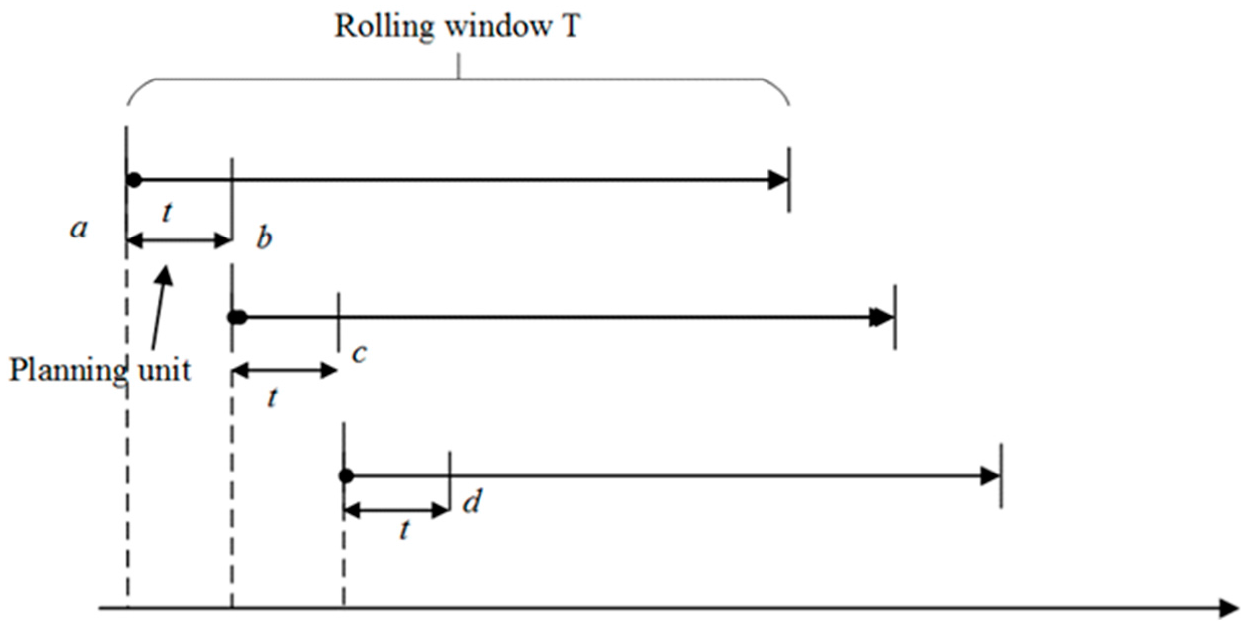
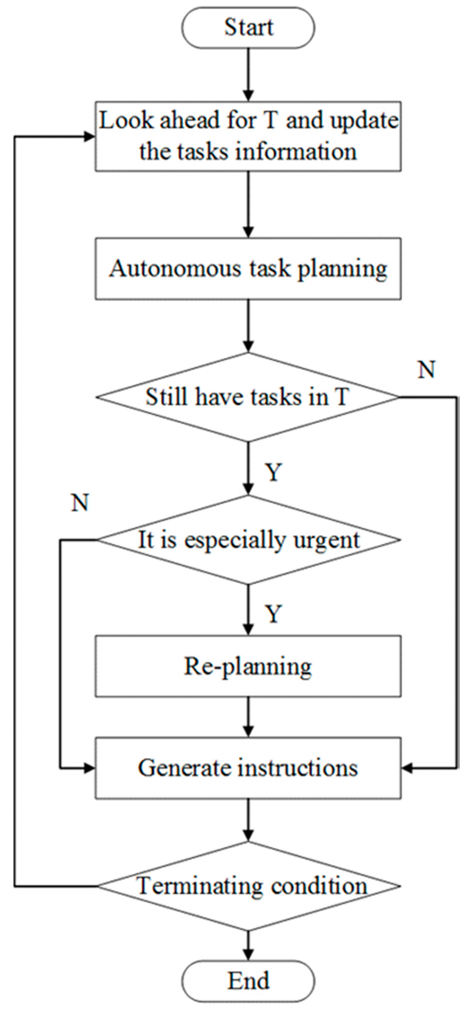
- Step 1: The length of a rolling window is T. Look ahead for T and update the tasks information in the rolling window. We also define a selected time t from the starting time of a rolling window as a planning unit. As shown in Figure 2.
- Step 2: Plan the tasks autonomously, the specific rules of the autonomous task planning are introduced in Section 3.2.
- Step 3: Check if there are still tasks to be arranged in the rolling window, and if so, return to the fourth step; if there is no task, then directly carry out the fifth step.
- Step 4: If the tasks are urgent, insert the tasks into the plan of the current rolling window based on the re-planning algorithm. If not, the sequence of tasks remains unchanged in the planning unit of the current rolling window, and the new tasks are planned in a new rolling window.
- Step 5: Execute the task sequence in the planning unit t, and scroll into the next round.
The process of autonomous task planning is shown in Figure 3.
3.2. Algorithm Design
In this paper, we propose an improved genetic algorithm. The improvements include the design of crossover and mutation operators for different individuals, and an improved roulette selection operator. The flowchart of the algorithm is shown in Figure 4.
3.2.1. Encoding Method
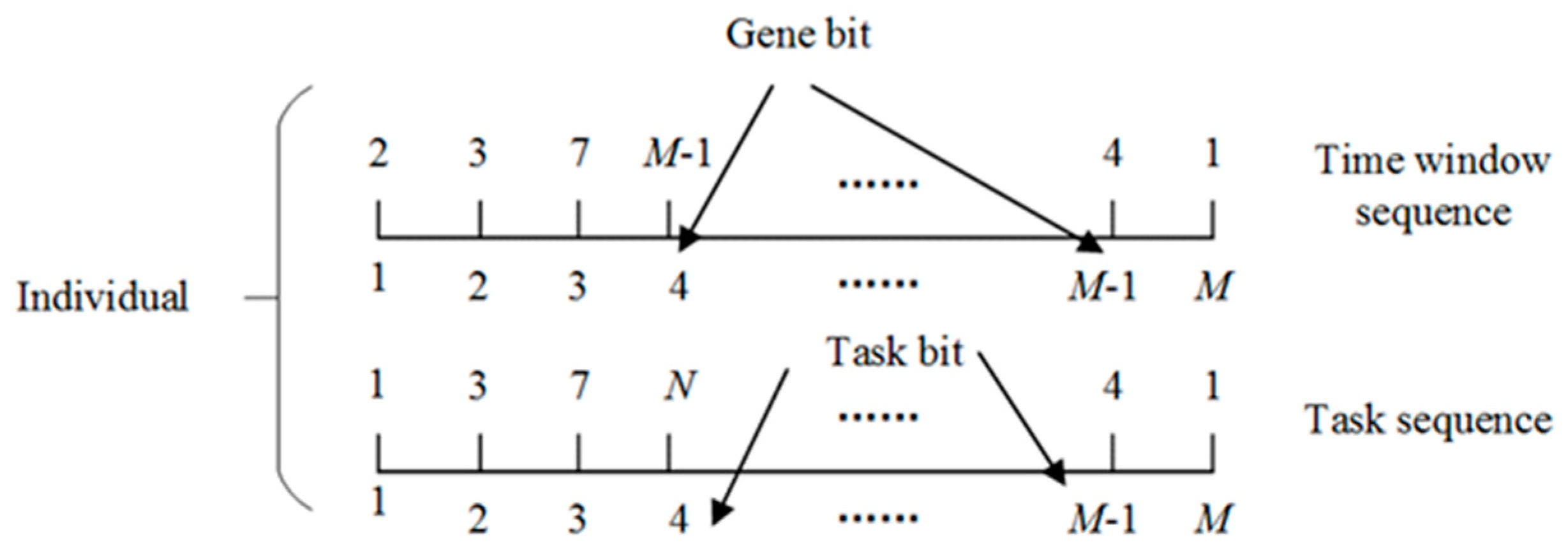
The genetic algorithm regards the solution of the problem as an individual or a population through the encoding process. We can get better individuals through the selection, crossover, and mutation process of the initial individual. The encoding forms are shown in Figure 5.
M and N respectively represent the number of time windows and the number of tasks needed to be planned. An individual is a matrix composed of integers. The value on the gene bit represents the corresponding time window. The value on the task bit represents the task number corresponding to the time window on the current gene bit. A task may have several time windows that can be selected, that is, a task number may correspond to several time windows. The initial population is generated randomly. For example, if M equals 5, N equals 3, it means that the number of time windows is 5, and the number of tasks is 3. An individual G may be encoded like this:
We can see that task1 corresponds to window1 and window3, which means that window1 and window3 are selected by task1, window5 is selected by task2, and window2 and window4 are selected by task3.
3.2.2. Selection Operator
In this paper, we use grouped roulette operators. The main steps are as follows:
- Step 1: Determine the number of population groups () and the number of all of the individuals ().
- Step 2: List all of the individuals in descending order of task profit.
- Step 3: Divide the sorted individuals into groups.
- Step 4: The group number of the i-th individual is as follows:
- Step 5: The probability that the i-th group is selected equals to the ratio of the total profit of the current group to the total population profit. Calculate the cumulative selection probability for each group to form a roulette.
- Step 6: Generate a random number within [0, 1], if the random number is greater than or equal to the cumulative probability of the (j − 1)-th group and is less than the cumulative probability of the i-th group, randomly choose an individual from the -th group as the returned individual.
The grouped roulette operator can be regarded as a trade-off between a traditional roulette operator and random selection. If equals the number of individuals in the population, it is the traditional roulette operator, and if is equal to 1, it is random selection. When applied, can be adjusted according to the actual problems, so that the grouped roulette operator can be continuous between the traditional roulette and random selection.
3.2.3. Cross and Mutation Operator
The crossover and mutation operator are used to optimize the initial population in order to generate individuals with higher fitness. According to the time constraints and resource constraints, we classify the individuals and analyze the possibility of increasing task profit, respectively, to guide the evolution of individuals.
We can get W and R through time constraints and resource constraints, respectively. The resource constraint checking is based on time constraint checking, thus the following conclusions can be drawn:
For example, the time window sequence of an individual is as follows:
is a M-dimensional vector, here is an example:
If the i-th time window can meet the time constraint, , otherwise, ; Therefore, according to the time constraints, the time window sequence that can be selected is .
is a M-dimensional vector, here is an example:
If the task of the i-th time window can meet the resource constraint, , otherwise, . Therefore, according to the resource constraints, the time window sequence that can be selected is .
We divide the individuals into two categories according to the point of view of whether W and are equal. If W is equal to , it indicates that all of the tasks that meet the time constraints are allocated to the required resources. Because of the small possibility of resources being used up, it can be considered that when W equals , there are resources that are left. Obviously, if the number of tasks satisfying the time constraints can be increased, it is possible to obtain more profitable individuals. In this case, there are also two states that can be subdivided according to whether the genome of an individual can fully meet the time-partially ordering constraint.
When the genome is not fully satisfied with the time partially order constraint, increasing the number of time windows that meet the time partially order constraint may result in more individuals with high returns. We call this state an under partially ordering state.
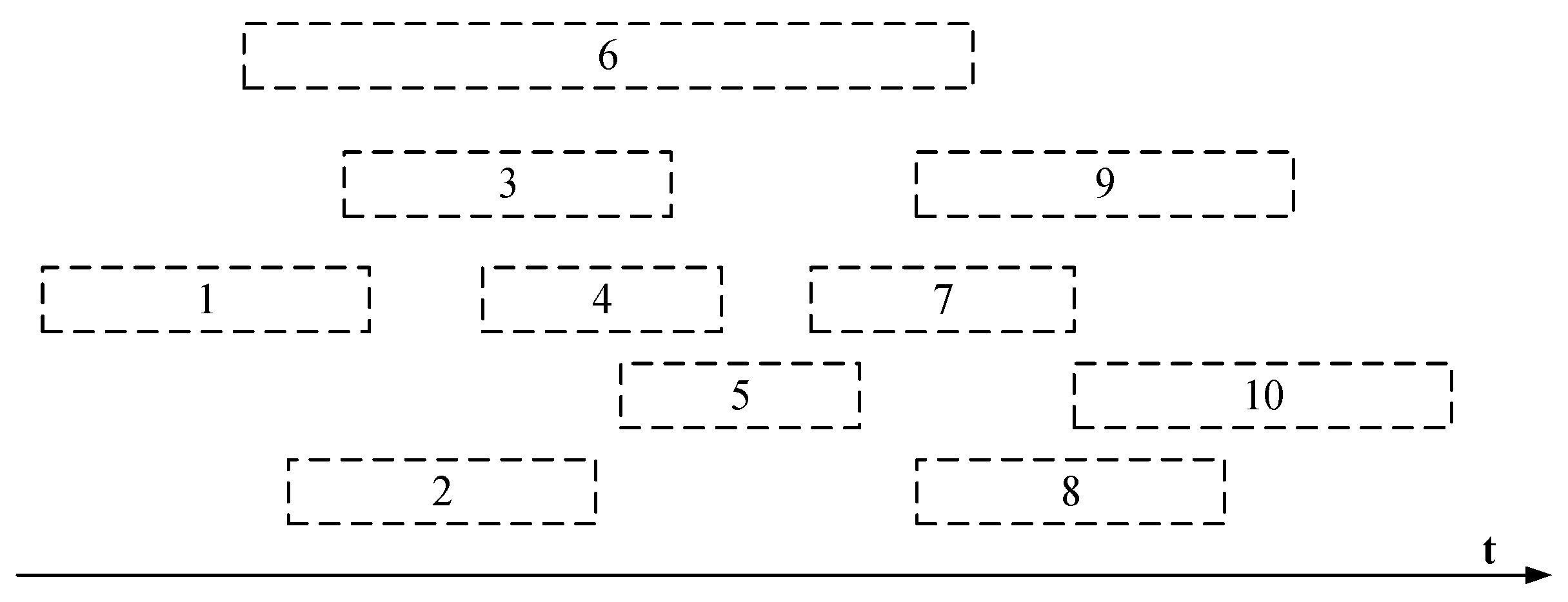
Here is an example of time partially order constraints, the relationship of the 10 time windows along the timeline is shown in Figure 6.
represents the set of time windows, ,. If , and , then . We call it a time partially order constraint. Taking as an example, the time windows that satisfy the time partially order constraint of is: ,, , , .
If two time windows do not satisfy Equations (10) and (11), we have defined that the two windows interact with each other, that is, interact with .
We define as the influence set of . . Let the time windows in the genome all meet the time constraints, that is . If a genome = [6, 1, 3, 4, 2, 7, 5, 9, 8, 10], according to the time constraint check rules, the selected genes are [1, 2, 5, 8, 10].
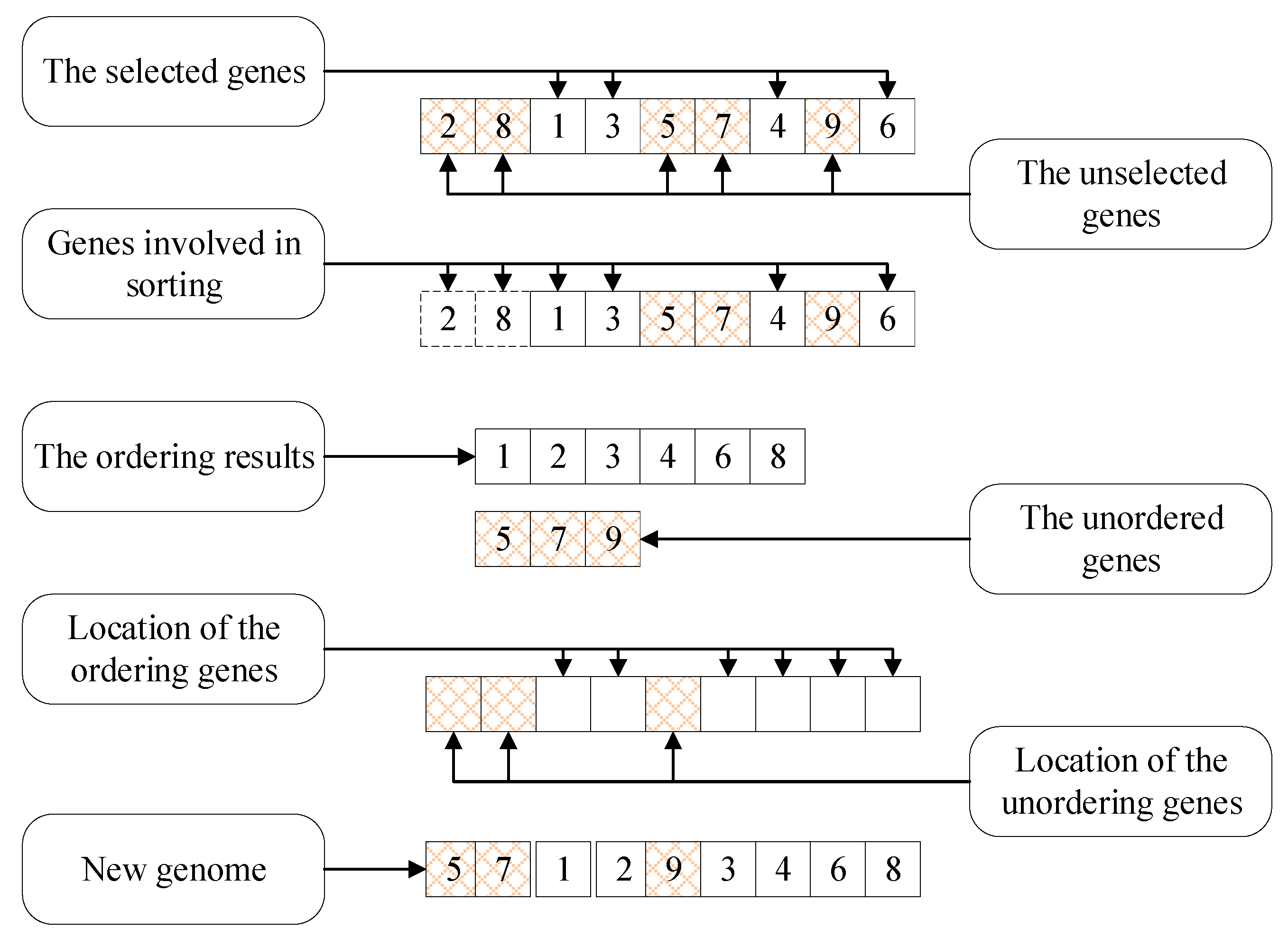
In order to improve the degree of the time partially order constraint, we propose a partially ordering mutation operator (TPOMO). The aim of TPOMO is to keep the original sequence of genes as long as possible, and to adjust the sequence of genes so that the new genome can meet the time partially order constraint. The steps of TPOMO are shown as follows:
- Step 1: Obtain an individual that is in line with this evolutionary direction.
- Step 2: Let be a set of genes selected by W in the genome, and let be a set of genes that are not selected by W in the genome. Choose and t genes from to form genotype1; the remaining genes in make up the genotype2.
- Step 3: Completely sort the genes of genotype1 in a time partially ordering, while the relative ordering of genotype2 remains unchanged.
- Step 4: Store genotype2 in the places that exclude the positions of the t genes, and store genotype1 in the positions of the t genes and the positions of the genes in to obtain a new genome.
The process of TPOMO is shown in Figure 7. For convenience, we assume that all of the time windows satisfy the time constraints.
The time partially ordering constraints can no longer contribute to increasing the number of tasks satisfying time constraints, when the genome fully satisfies the time partially ordering constraints. We call this state a fully partially ordering state.
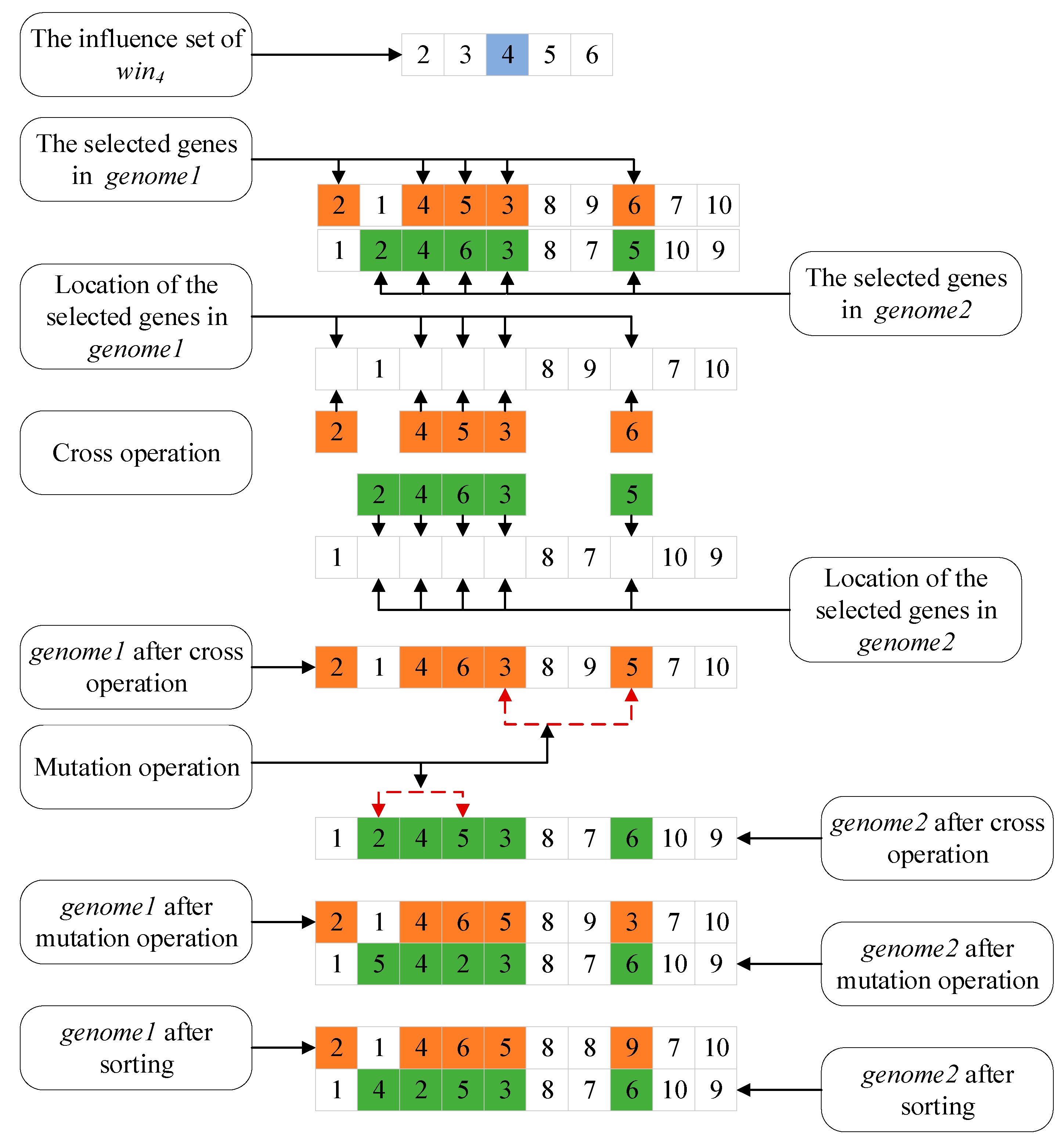
In this paper, we introduce new changes through crossover and mutation operations. The crossover and mutation operation can only be carried out within the influence set of the time windows. This is because the time windows in interact with . It is possible to generate new individuals by changing the ordering between the interacting windows so that the partial modification of the genome can be realized, while the genetic information of the rest of the genome can be preserved at the same time. In addition, we use the time partially ordering constraint to sort the new genomes in order, to ensure that the new individual still satisfies the time partially order constraint. Therefore, we propose an influence set crossover-mutation operator (ISCMO) to cross and mutate the genomes within the time window influence set, in order to obtain new individuals and to ensure that the new individuals fully meet the partially order constraints.
The steps of ISCMO is shown as below:
- Step 1: Obtain two individuals that are in line with this evolutionary direction.
- Step 2: Select , in turn, and perform the following crossover operations by probability. According to the original sequence, get from genome1 and genome2 to make up genotype1 and genotype2, respectively. Store genotype1 in the position of genotype2 and store genotype2 in the position of genotype1.
- Step 3: Select two genes from randomly, and exchange the position of these two genes in genome1. Then perform the same operation on genome2.
- Step 4: Sort genome1 and genome2 by time partially ordering to get new individuals.
The process of ISCMO is shown in Figure 8.
If W and are not equal, it indicates that not all task instances satisfying the time constraints are allocated to the required resources. That is, some task instances that meet the time constraints do not meet the resource constraints. We call it an insufficient state of resources.
Because of the limited allocation of resources within the planning time, there is no clear evolutionary direction at this time. We propose an inefficient time window crossover-mutation operator (ITWCMO) to solve this problem. The ITWCMO gives up the tasks with a low utilization of resources and selects new individuals with high resource utilization rates to improve the overall task income.
The steps of ITWCMO is shown as below:
- Step 1: Obtain two individuals that are in line with this evolutionary direction.
- Step 2: Calculate the absolute utilization efficiency of two kinds of resources for each gene of the two individuals, separately. The absolute resource utilization efficiency of a certain resource in a certain time window is equal to the income of the task to which the time window belongs, divided by the amount of the resource consumed.
- Step 3: Calculate the relative utilization efficiency of two kinds of resources, respectively. The relative resource utilization efficiency of a certain resource in a certain time window is equal to its absolute resource utilization efficiency, divided by the highest absolute resource utilization efficiency of the genes in the same individual.
- Step 4: Calculate the comprehensive relative resource utilization efficiency of each gene of the two individuals, separately. The comprehensive relative resource utilization efficiency of a certain time window is equal to the sum of its relative resource utilization efficiency of the two kinds of resources.
- Step 5: Perform the following operations on the two individuals. Select a gene, with the lowest efficiency of comprehensive relative resource utilization selected by and with the highest efficiency of comprehensive relative resource utilization selected by W, and not selected by . If the comprehensive relative resource utilization efficiency of is lower than that of , then rank in the first gene bit of genome.
- Step 6: Randomly select some genes to compose crossSet, according to probability.
- Step 7: According to the original sequence, extract the genes of crossSet sequentially from genome1 and genome2 to make up genotype1 and genotype2, respectively. Store genotype1 in the position of genotype2 and store genotype2 in the position of genotype1.
- Step 8: Select two genes from genome1 randomly and exchange the position of this two genes. Then, perform the same operation on genome2.
4. The Experiment and Analysis
The proposed algorithms are implemented by Satellite Tool Kit (STK) and Matlab2016a on a laptop with Core I7-6700HQ, 2.4 GHz CPU, 16 GB memory, and a Windows 10.1 operating system. In this study, the autonomous task planning of the small satellite within 24 h, and the dynamic changes of the task and satellite status were simulated, with a task profit range of 1–10.
In order to verify all of the crossover and mutation operators, we design four groups of experiments in this paper, with the degree of resource adequacy and time window overlapping as two variables. To investigate the performance of the improved genetic algorithms, this paper introduces a general genetic algorithm (GA) and improved genetic algorithm (IGA) as the core of the rolling-planning framework (step 2 in Figure 3), that is, the tasks are planned using a different task planning genetic algorithm in each group of experiments
The parameters of the rolling-planning framework are as follows:
- The length of the rolling window is two orbital cycles.
- The planning unit is half an orbital period.
The same data used in the four groups of experiments are the satellite orbit related data (as shown in Table 1) and Earth station related data (as shown in Table 2).
4.1. Performance Analysis of the Method
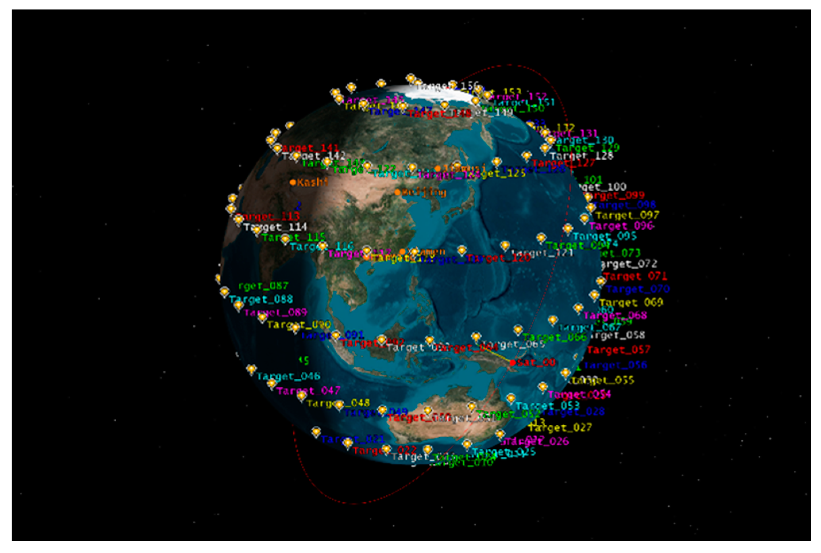
Experiment 1 and Experiment 2 are a group of comparative experiments. They compare the effects of different resource states on task scheduling under the same condition of low overlapping of time windows. We set 156 observation points evenly distributed on the nine dimensions of the Earth to simulate Experiment 1 and Experiment 2, as shown in Figure 9. The minimum elevation angle of the targets are random numbers between [50, 60].
In Experiment 1, resources are relatively abundant, and the specific parameters are set as follows. , the maximum storage capacity, equals 16 GB; the maximum electricity, , equals 5000 J; and the charge rate of satellite C equals 10 W. While in Experiment 2, equals 20,000 J, and C equals 5 W.
The parameters of the task in Experiment 1 and Experiment 2 are set as follows: the length of the execution time of the task obeys normal distribution, with the expectation of 120 s and the standard deviation of 20, the crossover probability is 0.3, the mutation probability is 0.5, the proportion of random individuals introduced into the new parent population is 0.15, the maximum number of iterations is 10, and the maximum population capacity is 30.
Experiment 3 and Experiment 4 are a group of comparative experiments too. They compare the effects of different resource states on task scheduling under the same condition of a high overlapping of time windows. The specific parameters of Experiment 3 are the same as those of Experiment 1, and the parameters of Experiment 4 are the same as those of Experiment 2.
The experimental arrangements can be summarized as follows.
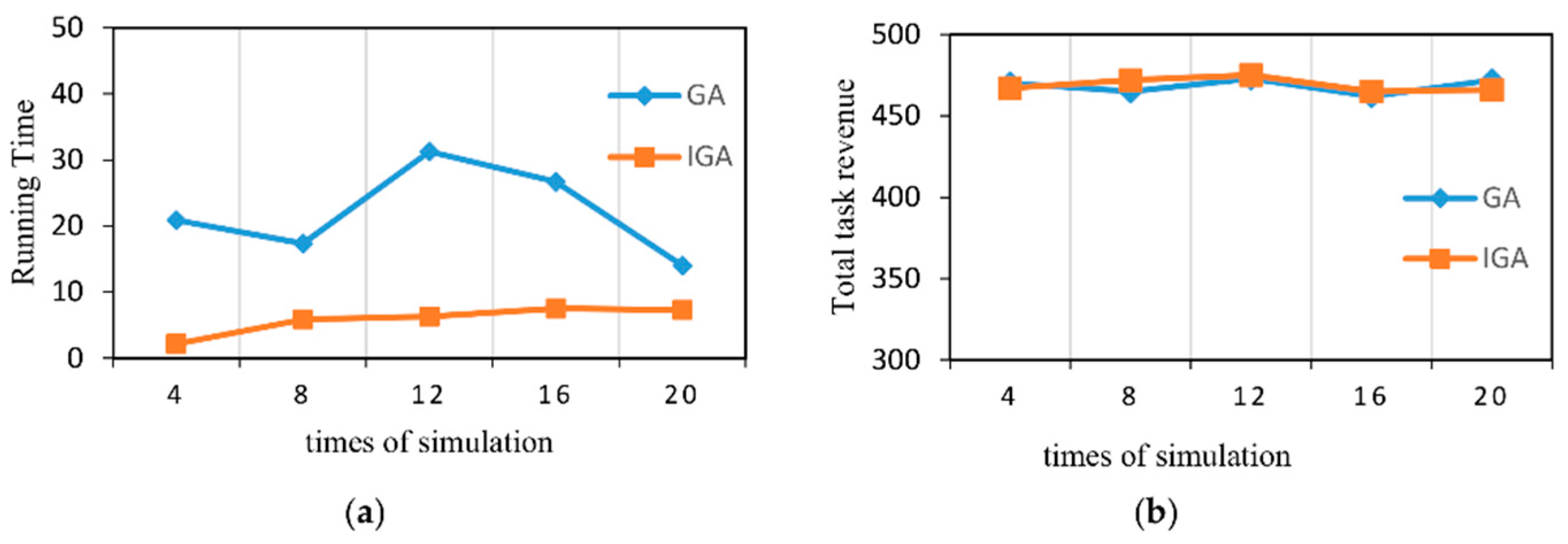
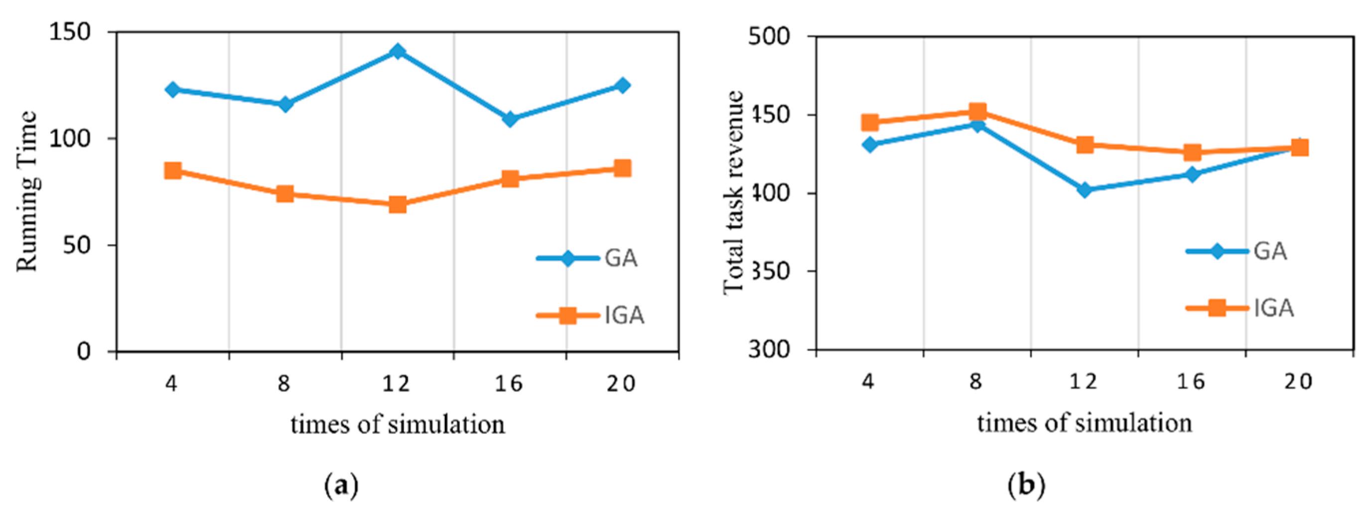
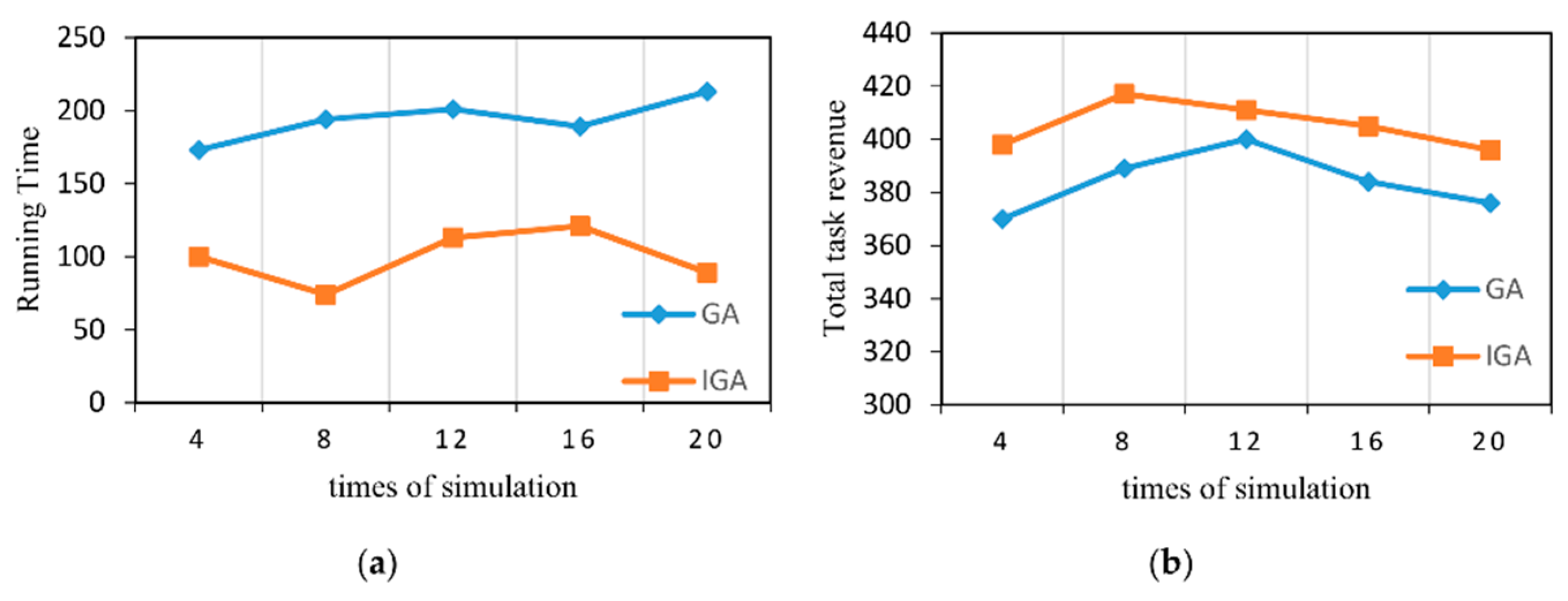
For the above four groups of experiments, the running time and the task revenue of the planning algorithm are shown in Figure 10, Figure 11, Figure 12 and Figure 13 respectively, after 20 times running.
In Experiment 1, both the time constraints and resource constraints are relatively loose. From Figure 10a,b, we can see that the maximum task revenue of GA and IGA are almost equal, but the running time of the IGA is only 50% that of the GA.
The time constraint in Experiment 2 is the same as that in Experiment 1, but its resource constraints are more stringent than Experiment 1. From Figure 11a,b, we can see that the income of the IGA is similar to that of GA. In terms of running time, IGA is superior in all running times, and its running time is about 25% that of GA.
In Experiment 3, the degree of the overlapping of time windows was high, while the resource constraints were relatively loose. It can be seen from Figure 12a,b that the average income of IGA is slightly higher than that of GA. In terms of the running time, the average running time of IGA is about 75% of the average running time of GA.
The time constraint in Experiment 4 is the same as that in Experiment 3, but its resource constraints are more stringent than Experiment 3. From Figure 13a,b, we can see that the income of the IGA is higher than that of GA. The average running time of IGA is about 50% of the average running time of GA.
Through the analysis above, we can know that IGA has shorter running time in the four groups of experiments, and IGA shows higher profit in Experiment 3 and Experiment 4. On the whole, IGA has the best performance in Experiment 4, the average running time is significantly better than that of GA, and the average income is also slightly better than that of GA. It can be concluded that IGA is more suitable for the task scenarios where the time constraints and resource constraints are stronger.
4.2. Stability Analysis of the Method
The comparison and summary of the running time and task total revenue of the four groups of experiments, after repeating 20 times, are shown in Table 3 and Table 4.
In the four groups of experiments, the distribution of the running time of IGA is more concentrated, and the average running time is significantly lower than that of GA. This phenomenon shows that IGA not only has a shorter average running time, but also has better stability than GA, in terms of running time.
In Experiment 1 and Experiment 2, the distribution of the total revenue of GA and IGA is basically the same, which shows that the two genetic algorithms are basically the same in terms of task revenue, when the time constraints are relatively loose.
In Experiment 3 and Experiment 4, IGA gains the highest revenue and has a more concentrated revenue distribution, which indicates that IGA has better stability in terms of task total revenue in the case of strict time constraints.
Through a comprehensive analysis of the above four groups of experiments, we can draw the following conclusions: In the case of the more relaxed time constraints, the two genetic algorithms are basically the same in revenue, and IGA has shorter running time. In the case of strict time constraints, IGA is not only superior to GA in running time, but also has better stability in terms of task revenue. Therefore, IGA is more suitable for onboard computation, because of the limited resources and computing power on board.
4.3. The Analysis of Task Execution Plan
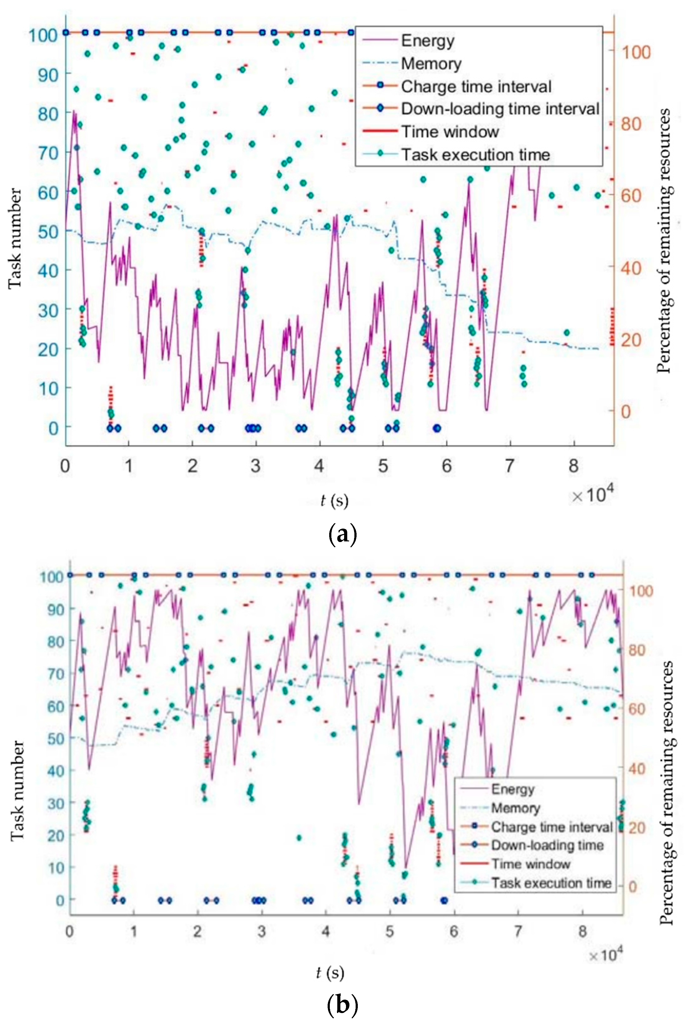
Figure 14a,b is the local task execution plans of IGA, which were randomly selected from Experiment 4. We chose Experiment 4 because in Experiment 4, the time constraints and resource constraints were more stringent, and the experimental results were more representative.
From Figure 14, we can see the following: (1) the battery energy fluctuates greatly, and it decreases rapidly in the area where the task execution intervals are intensive, which is in line with the actual law; (2) the battery energy recovers faster when the number of tasks is relatively small, and it can meet the needs of the task instances; (3) the memory has a small fluctuation on the whole; (4) the memory resources are released in the downlink interval, which is in line with the actual situation; (5) the tasks are executed in a coherent manner, which can prove that the algorithm can efficiently schedule dense tasks with time windows.
Therefore, we can make the conclusion that the proposed rolling–planning framework can achieve the continuous planning of satellite missions, which is of theoretical significance.
5. Conclusions
In this research, a model was established to solve the problem of the autonomous task planning of small satellites. With respect to the time constraint and dynamic resource constraint, this article conducts the research surrounding such issues in long-cycle task planning, and obtains the following research results.
With respect to the issue of continuous satellite task planning, this article designs a task planning framework based on rolling planning, and designs the rolling window and planning unit in the solution. For the satellite in-orbit application and with consideration of the limited onboard computing resource and time correlation, and resource correlation of the satellite task, this article puts forward an improved genetic algorithm. The algorithm adopts an individual coding rule based on fixed-length integer sequence coding, and encodes the task sequence to be planned with the fixed-length integer sequence, thereby narrowing down the search space; this article also categorizes each individual based on the compliance of individuals with time partial order constraint and resource constraint, and designs an appropriate crossover operator and mutation operator for each type of individual. By using task partial order sorting and individual categorization, it is possible to eliminate partial non-optimal individuals, narrow down the search space, and improve the computing efficiency of the algorithm. By using the adjustable grouping roulette operator, it is possible to realize the compromise between the traditional roulette operator and random selection operator, thus improving the premature issue of the genetic algorithm effectively. In addition, the article conducts the experimental verification on four sets of task scenarios. The results show the feasibility of the framework as proposed in this article and the validity of the algorithm.
Author Contributions
Conceptualization, J.L. and C.L.; formal analysis, C.L.; funding acquisition, J.L.; investigation, C.L.; methodology, J.L. and C.L.; project administration, C.L. and L.Z.; software, C.L. and L.Z.; supervision, S.C.; validation, S.C.; visualization, S.C.; writing (original draft), C.L. and L.Z.; writing (review and editing), J.L.
Funding
This research was funded by the National Natural Science Foundation of China (61272150, 61379110), and the Fundamental Research Funds for the Central Universities of Central South University (2018zzts062).
Acknowledgments
This work was supported in part by the National Natural Science Foundation of China (61472450, 61402165, 61702560, S1651002, M1450004), and the Key Research Program of Hunan Province (2016JC2018). The authors would like to thank the reviewers for their valuable suggestions and comments.
Conflicts of Interest
The authors declare no conflict of interest.
References
- Karapetyan, D.; Minic, S.M.; Malladi, K.T.; Punnen, A.P. Satellite downlink scheduling problem: A case study. Omega 2015, 53, 115–123. [Google Scholar] [CrossRef] [Green Version]
- Shimmin, R.; Schalkwyck, J.; Perez, A.D.; Weston, S.; Rademacher, A.; Tilles, A.; Agasid, J.; Burton, E.; Goktug, K.R.; Carlino, A. Small Spacecraft State of the Art Report 2015; NASA/TP-2015-21664; National Aeronautics and Space Administration: Moffett Field, CA, USA, 2016; pp. 68–133. [Google Scholar]
- Taleb, T.; Mashimo, D.; Jamalipour, A.; Kato, A.; Nemoto, Y. Explicit Load Balancing Technique for NGEO Satellite IP Networks With On-Board Processing Capabilities. IEEE/ACM Trans. Netw. 2009, 17, 281–293. [Google Scholar] [CrossRef]
- Sandau, R. Status and trends of small satellite missions for earth observation. Acta Astronaut. A 2010, 66, 1–12. [Google Scholar] [CrossRef]
- Beaumet, G.; Verfaillie, G.; Charmeau, M. Feasibility of Autonomous Decision Making on Board An Agile Earth Observing Satellite. Comput. Intell. 2015, 27, 123–139. [Google Scholar] [CrossRef]
- Chang, Z.X.; Li, J.F. Planning and scheduling of an agile earth observing satellite combining on-ground and on-board decisions. In Proceedings of the International Conference on Electrical, Automation and Mechanical, Engineering, Phuket, Thailand, 26–27 July 2015; pp. 530–533. [Google Scholar]
- Sherwood, R.; Chien, S.; Tran, D.; Cichy, B.; Castano, R.; Davies, A.; Rabideau, G. Intelligent Systems in Space: The EO-1 Autonomous Sciencecraft’ AIAA. In Hopkins University Applied Physics Laboratory: He; Springer: Berlin, Germany, 2005; pp. 26–29. [Google Scholar]
- Cichy, B.; Chien, S.; Schaffer, S.; Tran, D.; Rabideau, G.; Sherwood, R.; Mandl, D.; Bote, R.; Frye, S.; Trout, B.; et al. Validating the autonomous EO1 science agent. In Proceedings of the International Workshop on Planning and Schedule for Space, Darmstadt, Germany, 23–25 June 2004. [Google Scholar]
- Chien, S.; Tran, D.; Rabideau, G.; Schaffer, S.; Mandl, D.; Frye, S. Planning Operations of the Earth Observing Satellite EO-1: Representing and Reasoning with Spacecraft Operations Constraints. Available online: https://www.researchgate.net/publication/268295459_Planning_Operations_of_the_Earth_Observing_Satellite_EO-1_Representing_and_reasoning_with_spacecraft_operations_constraints (accessed on 10 July 2018).
- Davies, A.; Chien, S.; Baker, V.; Doggett, T.; Dohm, J.; Greeley, R.; Ip, F.; Castanǒ, R.; Cichy, B.; Rabideau, G.; et al. Monitoring active volcanism with the Autonomous Sciencecraft Experiment on EO-1. Remote Sens. Environ. 2006, 101, 427–446. [Google Scholar] [CrossRef]
- Chien, S.; Knight, R.; Stechert, A.; Sherwood, R.; Rabideau, G. Using iterative repair to improve the responsiveness of planning and scheduling. In Proceedings of the International Conference on Artificial Intelligence Planning Systems, Breckenridge, CO, USA, 14–17 April 2000; pp. 300–307. [Google Scholar]
- Verfaillie, G.; Bornschlegl, E. Designing and Evaluating an On-Line On-Board Autonomous Earth Observation Satellite Scheduling System. 2014–2015. Available online: http://robotics.estec.esa.int/IWPSS/IWPSS_2000/Papers/16.pdf (accessed on 10 July 2018).
- Song, Y.; Huang, D.; Zhou, Z.; Chen, Y. An emergency task autonomous planning method of agile imaging satellite. EURASIP J. Image Video Process. 2018, 2018, 29. [Google Scholar] [CrossRef] [Green Version]
- Luo, K.; Wang, H.; Li, Y.; Li, Q. High-performance technique for satellite range scheduling. Comput. Oper. Res. 2017, 85, 12–21. [Google Scholar] [CrossRef]
- Liu, W.; Li-Gang, L.I. Mission Planning of Space Astronomical Satellite Based on Improved Genetic Algorithm. Comput. Simul. 2014, 31, 54–58. [Google Scholar]
- Zhang, Y.; Xiang, M.; Zhang, H. An Improved Genetic Algorithm for Multi-satellite Tt&c Scheduling Problem. Infect. Dis. Poverty 2015, 5, 1–6. [Google Scholar]
- Miao, Y.; Wang, F.; Astronautics, S.O. Optimize-by-priority on-orbit task real-time planning for agile imaging satellite. Opt. Precis. Eng. 2018, 26, 150–160. [Google Scholar] [CrossRef]
- Liu, S.; Chen, Y.; Xing, L.; Guo, X. Time-dependent autonomous task planning of agile imaging satellites. J. Intell. Fuzzy Syst. 2016, 31, 1365–1375. [Google Scholar] [CrossRef]
- Li, Z.L.; Li, X.J.; Sun, W. Task Scheduling Model and Algorithm for Agile Satellite Considering Imaging Quality. J. Astronaut. 2017, 38, 590–597. [Google Scholar]
- Wu, J.; Liu, L.; Hu, X. A robust algorithm for deadline-constrained task scheduling in small satellite clusters. In Proceedings of the A robust algorithm for deadline-constrained task scheduling in small satellite clusters, Guilin, China, 12–15 June 2016; pp. 1769–1774. [Google Scholar]
- Chen, H.; Du, C.; Li, J.; Jing, N.; Wang, L. An approach of satellite periodic continuous observation task scheduling based on evolutionary computation. In Proceedings of the Genetic and Evolutionary Computation Conference Companion, Berlin, Germany, 15–19 July 2017; pp. 15–16. [Google Scholar]
- Zacharia, P.T.; Xidias, E.K.; Aspragathos, N.A. Task scheduling and motion planning for an industrial manipulator. Robot. Comput. Integr. Manuf. 2013, 29, 449–462. [Google Scholar] [CrossRef]
- Xidias, E.K.; Azariadis, P.N. Mission design for a group of autonomous guided vehicles. Robot. Auton. Syst. 2011, 59, 34–43. [Google Scholar] [CrossRef]
- Her, R.J.; Gao, P.; Bai, B.C. Models, algorithms and applications to the mission planning system of imaging satellites. Syst. Eng. Theor. Pract. 2011, 31, 411–422. [Google Scholar]
- Li, J.F.; Bai, B.C.; Chen, Y.W. Optimization algorithm based on decomposition for satellites observation scheduling problem. Syst. Eng. Theor. Pract. 2009, 29, 134–143. [Google Scholar]
- He, C.; Qiu, D.S.; Zhu, X.M. Emergency scheduling method for imaging reconnaissance satellites based on rolling horizon optimization strategy. Syst. Eng. Theor. Pract. 2013, 33, 2685–2694. [Google Scholar]
- Guo, H.; Qiu, D.S.; Wu, G.H. Tasks scheduling method for an agile imaging satellite based on improved ant colony algorithm. Syst. Eng. Theor. Pract. 2012, 32, 2533–2539. [Google Scholar]
- Vasquez, M.; Hao, J.K.A. “Logic-Constrained” Knapsack Formulation and a Tabu Algorithm for the Daily Photograph Scheduling of an Earth Observation Satellite. Comput. Optim. Appl. 2001, 20, 137–157. [Google Scholar] [CrossRef]
Figure 1.
Data-downloading tasks.

Figure 2.
The rolling process.

Figure 3.
The process of autonomous task planning.

Figure 4.
The flowchart of the improved genetic algorithm.

Figure 5.
A diagram of coding method.

Figure 6.
A diagram of 10 time windows.

Figure 7.
The mutation process of the time partially ordering mutation operator (TPOMO).

Figure 8.
The key steps of influence set crossover-mutation operator (ISCMO).

Figure 9.
The task scenery.

Figure 10.
The result of Experiment 1. (a) The running time of Experiment 1 and (b) the task revenue of Experiment 3.
Figure 10.
The result of Experiment 1. (a) The running time of Experiment 1 and (b) the task revenue of Experiment 3.

Figure 11.
The result of Experiment 2. (a) The running time of Experiment 2 and (b) the task revenue of Experiment 3.
Figure 11.
The result of Experiment 2. (a) The running time of Experiment 2 and (b) the task revenue of Experiment 3.

Figure 12.
The result of Experiment 3. (a) The running time of Experiment 3 and (b) the task revenue of Experiment 3.
Figure 12.
The result of Experiment 3. (a) The running time of Experiment 3 and (b) the task revenue of Experiment 3.

Figure 13.
The result of Experiment 4. (a) The running time of Experiment 4 and (b) the task revenue of Experiment 4.
Figure 13.
The result of Experiment 4. (a) The running time of Experiment 4 and (b) the task revenue of Experiment 4.

Figure 14.
(a) Local task execution plan and (b) local task execution plan.


Table 1.
Satellite orbit parameters.
| Semi-Major Axis | Eccentricity | Orbit Inclination Angle | Right Ascension of Ascending Node | Argument of Perigee | True Anomaly |
|---|---|---|---|---|---|
| 7878 km | 0 | 60° | 330° | 0° | 0° |
Table 2.
Ground Station Parameters.
| Ground Station | Longitude | Latitude | Minimum Angle of Elevation |
|---|---|---|---|
| Beijing | 116° | 40° | 20° |
| Kiamusze | 130.32° | 46.8° | 20° |
| Kashgar | 75.93° | 39.51° | 20° |
| Nanning | 108.37° | 22.82° | 20° |
| Xiamen | 118.09° | 22.48° | 20° |
Table 3.
Experimental arrangements.
| Experiment | Overlapping of Time Windows | Adequacy of Resources |
|---|---|---|
| Experiment 1 | Low | Yes |
| Experiment 2 | Low | No |
| Experiment 3 | High | Yes |
| Experiment 4 | High | No |
Table 4.
The running time and task total revenue of the experiments. SD—standard deviation.
| Experiment | Algorithm | Shortest/Average/Longest Running Time (s) | SD of Running Time (s) | Minimum/Average/Maximum Revenue | SD of Revenue | ||||
|---|---|---|---|---|---|---|---|---|---|
| Experiment 1 | GA | 1.72 | 2.37 | 4.63 | 1.57 | 514 | 514.2 | 516 | 0.61 |
| IGA | 0.83 | 1.03 | 2.1 | 0.36 | 514 | 514.1 | 516 | 0.45 | |
| Experiment 2 | GA | 14.01 | 20.88 | 31.56 | 8.47 | 462 | 470 | 479 | 5.03 |
| IGA | 2.19 | 5.31 | 9.73 | 2.56 | 463 | 470 | 478 | 4.83 | |
| Experiment 3 | GA | 107.3 | 122.5 | 153.3 | 39.56 | 397 | 420 | 453 | 23.52 |
| IGA | 69.1 | 85.7 | 98.4 | 20.17 | 417 | 431 | 463 | 18.57 | |
| Experiment 4 | GA | 173 | 189 | 217 | 34.17 | 352 | 383 | 405 | 21.92 |
| IGA | 74.5 | 99.7 | 121 | 17.79 | 380 | 409 | 437 | 18.51 | |
© 2018 by the authors. Licensee MDPI, Basel, Switzerland. This article is an open access article distributed under the terms and conditions of the Creative Commons Attribution (CC BY) license (http://creativecommons.org/licenses/by/4.0/).
Share and Cite
MDPI and ACS Style
Long, J.; Li, C.; Zhu, L.; Chen, S.; Liu, J. An Efficient Task Autonomous Planning Method for Small Satellites. Information 2018, 9, 181. https://doi.org/10.3390/info9070181
AMA Style
Long J, Li C, Zhu L, Chen S, Liu J. An Efficient Task Autonomous Planning Method for Small Satellites. Information. 2018; 9(7):181. https://doi.org/10.3390/info9070181
Chicago/Turabian StyleLong, Jun, Cong Li, Lei Zhu, Shilong Chen, and Junfeng Liu. 2018. "An Efficient Task Autonomous Planning Method for Small Satellites" Information 9, no. 7: 181. https://doi.org/10.3390/info9070181
Note that from the first issue of 2016, this journal uses article numbers instead of page numbers. See further details here.