Construction of Complex Network with Multiple Time Series Relevance

Abstract

Multivariate time series data, which comprise a set of ordered observations for multiple variables, are pervasively generated in weather conditions, traffic, financial stocks, etc. Therefore, it is of great significance to analyze the correlation between multiple time series. Financial stocks generate a significant amount of multivariate time series data that can be used to build networks that reflect market behavior. However, traditional commercial complex networks cannot fully utilize the multiple attributes of stocks and redundant filter relationships and reveal a more authentic financial stock market. We propose a fusion similarity of multiple time series and construct a threshold network with similarity. Furthermore, we define the connectivity efficiency to choose the best threshold, establishing a high connectivity efficiency network with the optimal network threshold. By searching the central node in the threshold network, we have found that the network center nodes constructed by our proposed method have a more comprehensive industry coverage than the traditional techniques to build the systems, and this also proves the superiority of this method.

1. Introduction

In the real world, a large number of systems can be described by complex networks [1,2,3,4]. The financial market is naturally a complex system, and the economy and financial systems have a self-organized complexity [5]. Many studies have shown that complex networks have been successfully used to describe financial systems [6]. From a different point of view, people put forward much network construction arithmetic [7,8,9]. In the U.S. stock market, the power-law of the degree distribution [10] in the minimum spanning tree (MST) has been observed [11]. The minimum spanning tree and hierarchical tree are also used to study the topology of correlation networks among major currencies [12,13] and financial crisis [14]. Kwapień et al. [15] introduced a family of q-dependent minimum spanning trees (qMSTs) that are selective for cross-correlations between different fluctuation amplitudes and different time scales of multivariate data. Djauhari et al. [16] introduced a set of optimality criteria and proposed the process of selecting the optimal MST. Through the analysis of the planar maximally-filtered graphs (PMFG) of the portfolio of the 300 stocks traded, Tumminello et al. [17] confirmed that the selected stocks composed a hierarchical system progressively structuring as the sampling time horizon increases. The method of correlation networks has been applied to the structural transition of financial systems during a crisis in a local market [18]. In the Tehran stock market and the DJIA, a scale-free threshold network in a restricted threshold has been observed [19]. Longfeng Zhao et al. [20] found some long-duration edges that serve as the backbone of the stock market during crises. Huang Weiqiang et al. [21] used the threshold method (traditional method) to construct Chinese stock-related networks and then studied the structural properties and topological stability of the net.

In common cases, the information on parts of the dynamical system is expressed in the form of time series, and time series analysis is a classic means of data analysis [22]. Recently, there has been a growing industry in the application of complex network theory to carry out time series analysis [23,24]. The time series firstly is transformed into networks and then analyzed with various complex network tools [25,26,27,28]. Shirazi et al. [29] demonstrated that the time series can be reconstructed with high precision by means of a simple random walk on their corresponding networks. The interaction of financial markets naturally constitutes a complex system in which the stock data are a multivariate time series (MTS) [30] of information in each part of the complex system. RN Mantegna [31] mapped the financial market as a network, the vertices of which are stocks and the edges between vertices are the relationships of shares. Kazemilari et al. [32] constructed a multivariate correlation network of stocks where each of them was represented by a multivariate time series, and vector correlation was used to measure the similarity among multivariate time series in the stock network.

Although networks based on price fluctuations can help us understand the complex correlations between stocks, the direct conversion implicitly assumes the Markov property (first-order dependency) and loses important information about dependencies in the raw data. Besides, the stock market constructed with the volatility relationship of the closing price data ignores other attributes of the stock, which are the multivariate time series. In real life, simple price fluctuations do not support a series of other data, such as trading volume, and the impact of stock fluctuations cannot effectively pass this effect on to related stocks. Therefore, the stock price fluctuation network constructed by the closing price time series cannot fully portray the interoperability between the time series itself and make full use of the stock’s multi-attribute information.

Due to the limitations of the stock price index correlation threshold network, we will introduce and improve a new method of building a stock network. First of all, we select a representative multiple sub-time series from a multi-stock time series and convert each sub-time series into a Gramian angular field (GAF) [33] grayscale image. We then merge multiple GAF grayscale images into MGAF color images and construct a multivariate stock network by calculating image similarity. Finally, we find that the network established by our method has a high connectivity efficiency, and the central node has wider industry coverage than the network constructed by the stock price index correlation threshold method. Next, we will introduce the network construction method in detail and give the empirical research and results in the summary.

2. Image Fusion Network Construction Method

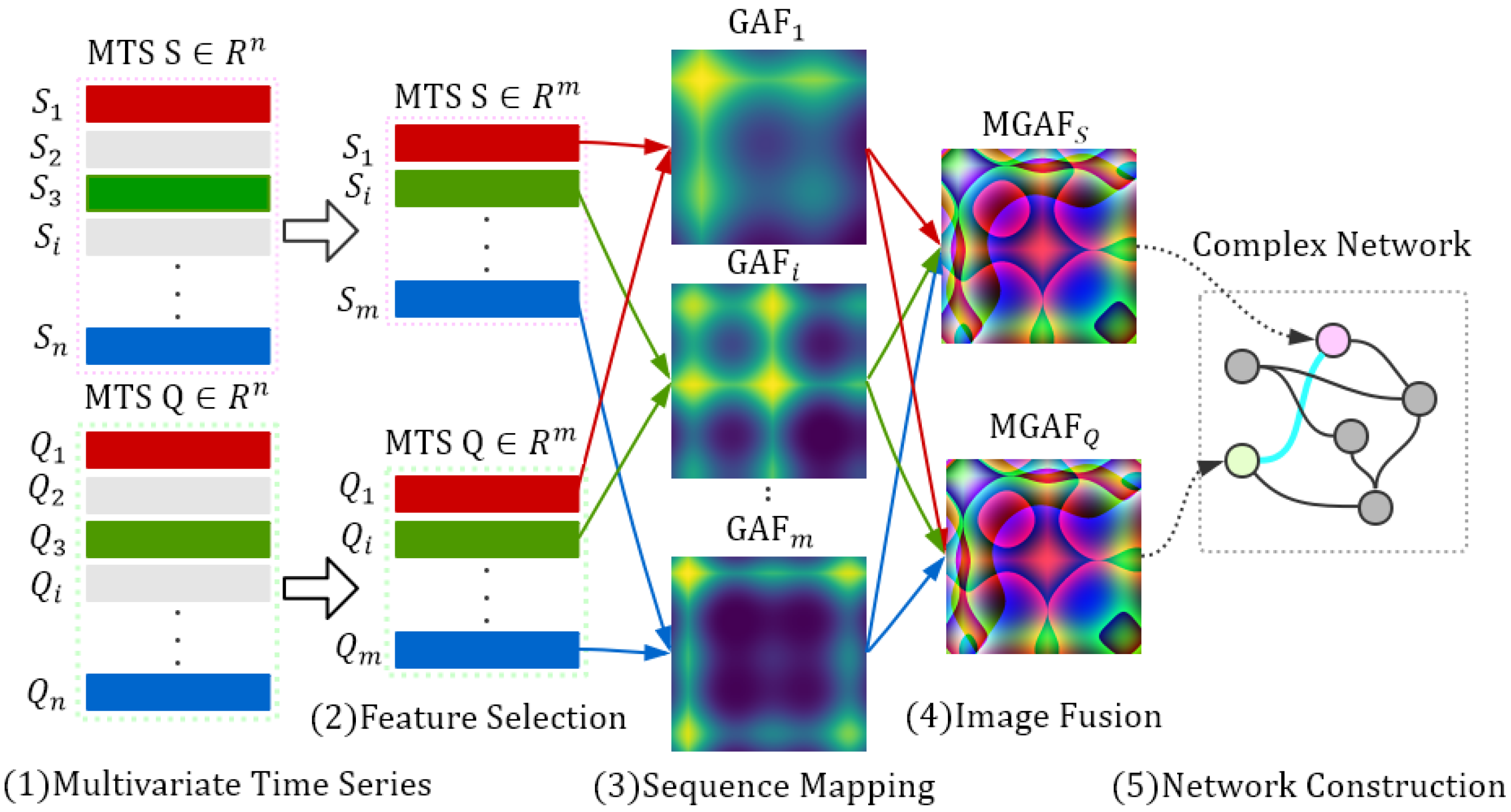
In this section, we will introduce how to construct complex networks using multivariate time series. The process is as shown in Figure 1.

2.1. Feature Selection

An MTS contains a set of ordered observations at a discrete time for multiple variables. To reduce the amount of computation while retaining as much information as possible, we use the Pearson correlation coefficient to perform feature selection on MTS. The Pearson correlation coefficient between each subsequence of multiple time series $X_i$ is as Equation (1).

$${\rho }_{x_i,x_j}=\frac{cov\left(X_i,X_j\right)}{{\sigma }_{x_i}{\sigma }_{x_j}}$$

(1)

where $X_i$ is the sequence of the i-th attribute of the time series X, ${\sigma }_{x_i}$ is the standard deviation of $X_i$ and $cov\left(X_i,X_j\right)$ is the covariance of the $X_i$ and $X_j$. The elements ${\rho }_{x_i,x_j}$ are restricted to the interval [−1, 1], where ${\rho }_{x_i,x_j}=1$ defines perfect correlation and ${\rho }_{x_i,x_j}=-1$ corresponds to perfect anti-correlation. ${\rho }_{x_i,x_j}=0$ corresponds to uncorrelated pairs of stocks.

2.2. Imaging Multivariate Time Series and Similarity Calculation

The GAF [33] converts time series $X_i=\left(x_{i1},x_{i2}\dots x_{in}\right)$ into grayscale images. The GAFs provide a way to preserve temporal dependency, since time increases as the position moves from top-left to bottom-right. The GAFs contain temporal correlations because $G_{(i,j||i-j|=k)}$ represents the relative correlation by superposition of directions for time interval k. In contrast, GAFs are essentially grayscale images that represent only the time series of a single attribute. Considering many time series, such as stocks, have multiple attributes, we propose that multiple GAFs be defined as Equation (2).

$$MGA{F}_m=\sum _{i=1}^m{w}_i·G_i=w^{\top }·G$$

(2)

where $G_i$ is an $n\times n$ pixel GAFs image converted from subsequence $X_i$ and $w_i$ is the fusion weight corresponding to the grayscale image $G_i$. $MGA{F}_m$ is an image fused by m GAF images.

In the construction of correlation threshold networks, we often need to know the size of the differences between individuals and then evaluate the similarity between individuals. Through the method described above, we converted each stock into an image. Then, we calculated the image similarity to determine the network edge. Fortunately, the structural similarity (SSIM [34]) is excellent in image similarity. The structural similarity index defines the structural information from the perspective of image composition as a property that reflects the structure of the object in the scene independently of the brightness and the contrast and models the distortion as a combination of the three different factors of brightness, contrast and structure. The mean value is used as the estimate of brightness; the standard deviation is used as an estimate of contrast; and the covariance is used as a measure of the degree of structural similarity. We use Equation (3) to evaluate the overall image similarity.

$$MSSIM\left[M_i,M_j\right]=\frac{1}{N}\sum _{n=1}^{N}SSIM\left[M_{in},M_{jn}\right]$$

(3)

where the images $M_i$ and $M_j$ are divided into N sub-images in the same manner.

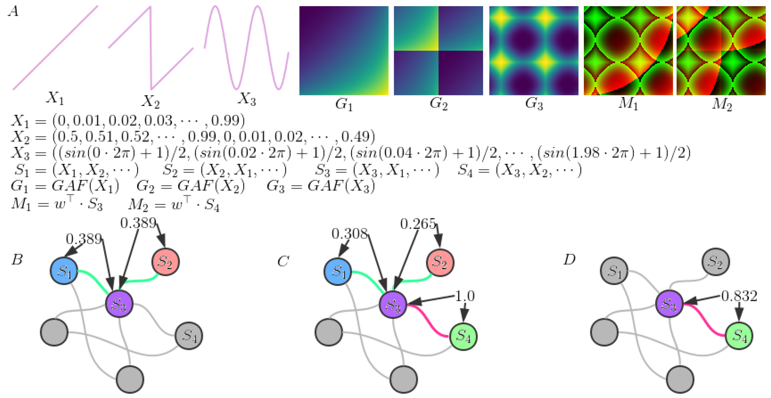
Suppose $S_i=\left(S_{i1},S_{i2},\cdots \right)$ represents stock i, where $S_{i1}$ represents the closing price sequence and $S_{i2}$ represents the turnover rate sequence. $S_1$, $S_2$, $S_3$ and $S_4$ are four different stocks, and we can see the different correlation of these stocks in Figure 2. For the stock Pearson cross-correlation methods that usually only focus on the closing price of a stock [21], $S_3$ and stock $S_1$ have the same absolute value of the Pearson similarity of stock $S_3$ and stock $S_2$. GAF images take into account the time dependence of time series, and stock $S_3$ and stock $S_1$ have the different $MSSIM$ of stock $S_3$ and stock $S_2$. The $MSSIM$ of stock $S_3$ and stock $S_1$ is 0.308; the $MSSIM$ of stock $S_3$ and stock $S_2$ is 0.265. Considering only the closing price of the stock, the $MSSIM$ of stock $S_3$ and stock $S_4$ is 1.0. The $MSSIM$ of stock $S_3$ and stock $S_4$ is 0.832, taking into account the stock closing price and turnover rate. With the appropriate thresholds, the fused image of the stock can distinguish the previous one, while the traditional method [21] cannot distinguish this. This is the advantage of converting a multivariate time series into a fused image.

2.3. The Connection Efficiency

In order to understand the features of the similar structure of financial stocks better, we establish the stocks’ associated networks (SAN) using complex network theory. To observe the network attributes under different thresholds in a more intuitive way, we define the connection efficiency in addition to the common network global attributes such as the average clustering coefficient [35], the average efficiency [36], density and the fraction of the coverage.

Network density can be used to characterize the degree of a respective edge between nodes in the network. It is defined as Equation (4).

$$D=\frac{2m}{n\left(n-1\right)}$$

(4)

where n is the number of nodes and m is the number of edges in the network.

In an undirected graph G, $v_i$ and $v_j$ are connected if there is a path from vertex $v_i$ to vertex $v_j$. A maximally-connected subgraph of an undirected graph G is called a connected component of G. The ratio between the maximum number of connected component nodes and the number of stocks in a network is then defined as the fraction of the coverage of the network, that is Equation (5).

$$F=\frac{S_{max}}{\left|V\right|},S=\left\{\left|V_i\right|,V_i\subset V\right\}$$

(5)

where V is the collection of stocks in a network and $V_i$ is the collection of the connected component of a stock network.

The connection efficiency can be used to characterize the strength of edge connection nodes. According to Equation (6), if we want to maximize the connection efficiency, we need to the fraction of the coverage (F) of the network as much as possible and minimize the network density (D). Looking back at Equations (4) and (5), we will build a network whose edges link all nodes as much as possible without making the edges too dense. In other words, we use fewer edges to get more nodes to access the network. The higher the connection efficiency, the stronger the ability of the edge to connect to the node. This means that, compared to the previous network construction methods, the connected edges found by our proposed method are more important, and the relationship between stocks is more significant.

$$CE=F-D$$

(6)

where D is the network density and F is the fraction of the coverage of the network.

3. Results and Discussion

3.1. Data

The data used in this article were from the Tushare Financial Data Interface (http://tushare. org/). The selected data included the CSI 300 constituent stocks for 100 trading days from 30 March 2017 to 22 August 2017. As some stocks suspended, we preprocessed the data and finally left the transaction data in 279 stocks. Financial indicators included open (open price), high (highest price), close (close price), low (lowest price), volume (volume), price_change (change), p_change (%Chg), ma5 (five-day average price), ma10 (10-day average price) ma20 (20-day average price), v_ma5 (5-day average volume), v_ma10 (10-day average volume), v_ma20 (20-day average volume) and turnover (turnover rate).

3.2. The Network Overview

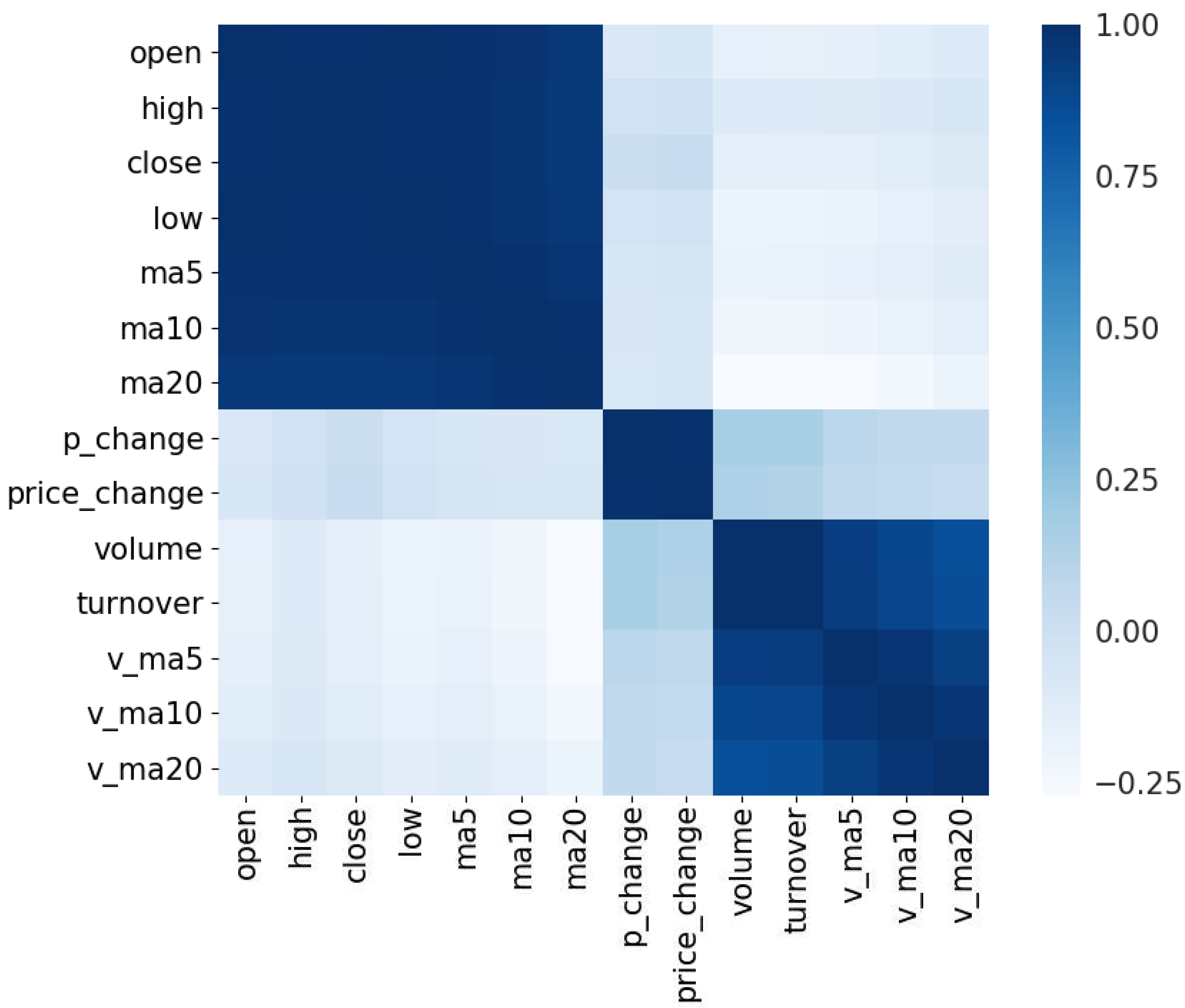
We calculate the Pearson correlation coefficient between the stocks’ properties. Through Figure 3, we can see that the attributes are roughly divided into three groups, so we choose $m=3$.

The $MGA{F}_3$ formula is as Equation (7).

$$MGA{F}_3=\sum _{i=1}^3{w}_i·G_i=w^{\top }·G$$

(7)

where $G=\left(G_1,G_2,G_3\right)$ is the GAF image converted from ups and downs, closing price and the turnover rate respectively and $w^{\top }={\left(0.299,0.587,0.114\right)}^{\top }$ is the fusion weight. We used the default parameter values that the RGB image converted to the grayscale image as fusion weights, but this is not limited to this kind of weight. One can modify the weights according to one’s needs to get different results.

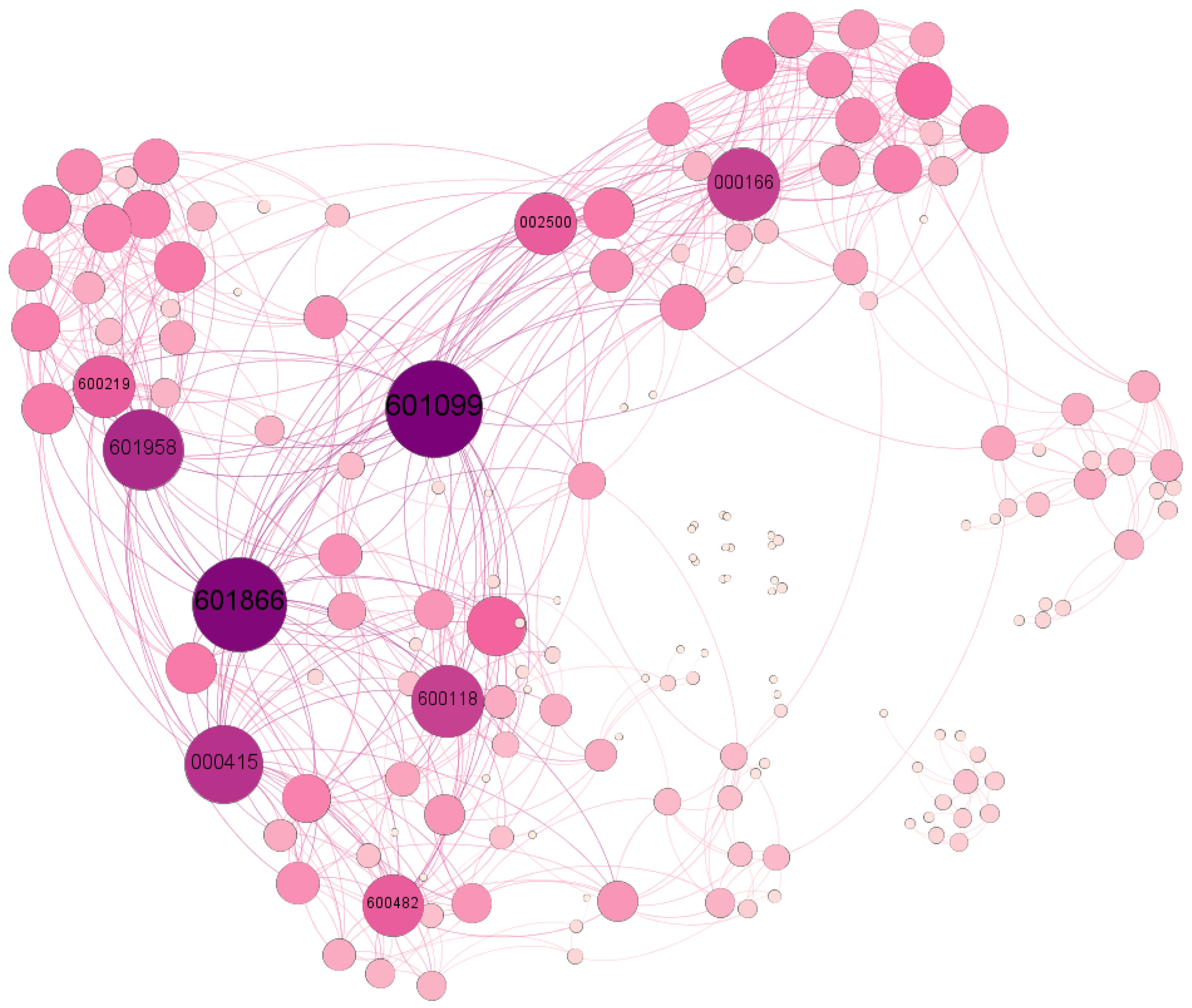
Then, we calculated the image similarity $MSSIM$ and established SAN models with different thresholds. Then, we selected the appropriate threshold network as a representative, as shown in Figure 4. The size of each node depends on the degree of the node.

3.3. Threshold Selection

For building a correlation threshold network, how to choose a reasonable threshold is the key. At present, the threshold is determined based on a comparison of attributes between different threshold networks; or the threshold is set based on relevant expert experience. To explore how to determine the threshold of the network, we constructed the fibers with different thresholds of 0.01 to 0.86 and statistics; the global properties of the system by each limit are shown in Figure 5. From the local features of the network, the role of nodes in the system is very different. A few critical nodes played a leading role in the operation of the network. We compared the node centrality of the system within the threshold interval and ranked the first ten nodes according to their centrality, as shown in

Table 1. Degree centrality in the image similarity stock network.

0.1	0.15	0.2	0.25	0.3	0.35	0.4	0.45	0.5	0.55
000623	601099	601099	601099	601099	601958	601958	601958	600118	601390
000031	000166	601866	601866	601866	601866	000166	000166	600030	601958
000166	000623	000166	000415	601958	600118	601555	600999	601390	300027
601099	601881	000415	601958	000415	000166	600118	601688	601958	600219
001979	000157	002500	600118	600118	601099	600999	600030	600340	300251
601881	002736	600118	002500	000166	601555	601788	601390	600999	600999
600585	600221	600958	000166	600219	600219	600482	601788	601688	601766
600340	000415	601881	600583	002500	600482	600030	600118	601818	601997
000008	600118	600583	600038	600482	600030	000060	600837	300027	600919
000157	601866	601958	600958	600038	000415	601866	601555	600219	601998

and

Table 2. Degree centrality in the Pearson stock network.

0.1	0.2	0.3	0.35	0.4	0.45	0.5	0.6	0.7	0.8
601555	000166	000686	000686	000686	000686	000686	601555	601555	601788
002736	000686	000166	000166	000166	601555	601555	601788	601788	000686
000166	002736	000157	601555	601555	000166	000166	002736	002736	601555
600369	000783	601555	600909	002500	601163	601099	000686	600030	600909
000686	002500	600369	000157	601163	002500	002736	000783	600999	601375
600909	601555	002500	002500	600369	601099	600999	600030	000686	601186
600958	000157	600909	601099	002736	600369	601788	000166	000166	000783
601099	600369	601099	002736	601099	600909	600369	601198	000783	601881
002470	600498	002736	600369	000157	601375	002500	600999	002500	000166
600030	002081	601881	601163	603858	002736	000783	601099	600369	601390

.

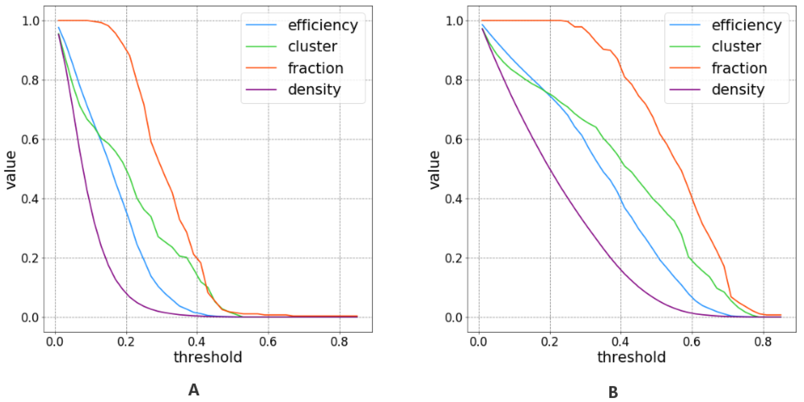
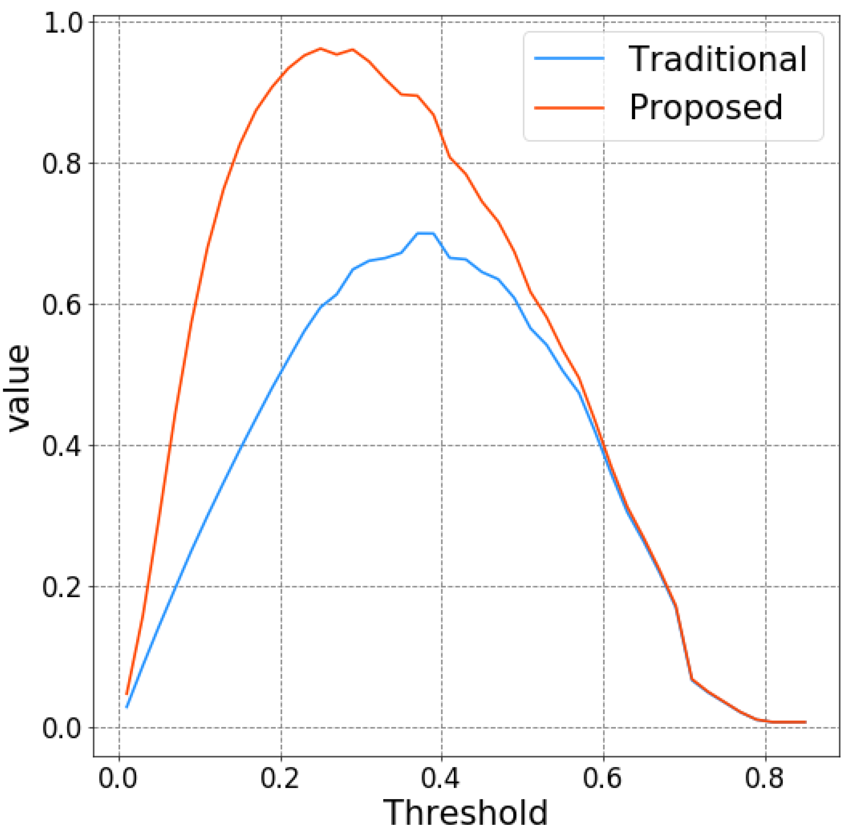
From Figure 5, we can see that as the threshold increases, the network density, the average clustering coefficient, etc., are continuously decreasing. We can imagine that when the threshold is too small, there is an edge between almost all nodes, which is equivalent to a complete graph. However, when the limit is too large, almost all nodes are isolated. To reduce redundant edges and incorporate all nodes into the network as much as possible, we defined the connection efficiency and chose the limit that maximized the connectivity efficiency as the network’s threshold. As shown in Figure 6, we see that the connection efficiency rises steeply within the threshold interval, reaching a rapid drop after a rare extreme.

From the table, we can get that the first row in the table represents the threshold, and each column in the table shows the node code with a larger degree centrality at this threshold. Observing the table horizontally, we have found that no matter how the threshold changes, there are always some nodes that are always more central nodes, which are more important nodes. Looking at the table longitudinally, we find that some thresholds contain fewer important nodes, whereas some thresholds contain more important nodes. We think that the threshold contains a greater number of important nodes, that it is more appropriate it is and that we want it to be more so. In order to facilitate the observation of the frequency of stocks, we mark the stocks in the table in red, purple, green, blue and white in order of frequency. From the table, we can see that the high-order nodes of the network constructed by our method tend to have a threshold of 0.3. Similarly, high-order nodes of a network built by the stock price index correlation threshold method (traditional method) tend to have a threshold of 0.4. Concerning Figure 6, Table 1 and Table 2, we can conclude that when the value of connectivity efficiency is more significant, the number of high-frequency center nodes increases, and when the connection efficiency reaches a maximum value, the number of high-frequency center nodes is the highest. This shows that the network constructed near the maximum of the connectivity efficiency can better characterize the relationship between stocks, and from the side, our defined threshold selection criteria, the connectivity efficiency, can help us to select the appropriate threshold. Moreover, as can be seen from Figure 6, the effectiveness of the network constructed by the method proposed by us is higher overall than the traditional method. However, as can be seen from Table 1 and Table 2, the number of network high-frequency center nodes constructed by this method is generally lower than the traditional method. This means that the network we have built uses fewer edges to achieve higher connection efficiency and better reflects the indispensable interaction between stocks.

In addition, we also found that the vast majority of the stocks (000166, 000686, 601555, 600369, 002736, 601099, 002500, 600909, 000783) of nodes with relatively high degrees of the network constructed by traditional methods belong to the financial industry. The stocks (600118, 601958, 000166, 601866, 601099, 000415, 600482, 600219) corresponding to the nodes with higher networks moderately constructed by our method belong to the communication equipment, mining industry, financial industry, transportation logistics and non-ferrous metals, metals, shipping equipment, leasing and commerce, respectively. This has important implications for our study of the relationship between different industries in the entire stock market. Although the model presented in this paper has achieved good experimental results, there are still some shortcomings. Because of the calculation of image similarity, the algorithm is not efficient. What is more, the system is an undirected network, which does not reflect the typical asymmetric interactions in the real world.

4. Conclusions

This paper selects the characteristics of multivariate stock sequences, converts the critical attribute sequences into grayscale images to compose color images and calculates the similarity between images. In fact, we proposed a way to calculate the correlation of multivariate time series. We treat the stock as a node, consider the relationship between the shares corresponding to the images as a continuous edge and build a stock network based on different thresholds. Furthermore, we define the connectivity efficiency to choose the best limit and establishing a high connectivity efficiency network with the optimal network threshold. By searching the central node in the threshold network, we have found that the network center nodes constructed by our proposed method have a more comprehensive industry coverage than the traditional techniques to build the systems, and this also proves the superiority of this method. Creating a directed net and popularizing our algorithm model in more realistic systems will be our future research direction.

References

- Newman, M.E.J. The Structure and Function of Complex Networks. SIAM Rev. 2003, 45, 167–256. [Google Scholar] [CrossRef] [Green Version]
- Albert, R.; Barabási, A. Statistical mechanics of complex networks. Rev. Mod. Phys. 2002, 74, 47. [Google Scholar] [CrossRef]
- Guimera, R.; Amaral, L.A.N. Functional cartography of complex metabolic networks. Nature 2005, 433, 895–900. [Google Scholar] [CrossRef] [PubMed] [Green Version]
- Boccaletti, S.; Latora, V.; Moreno, Y.; Chavez, M.; Hwang, D.U. Complex networks: Structure and dynamics. Phys. Rep. 2006, 424, 175–308. [Google Scholar] [CrossRef] [Green Version]
- Stanley, H.E.; Amaral, L.A.N.; Buldyrev, S.V.; Gopikrishnan, P.; Plerou, V.; Salinger, M.A. Self-Organized Complexity in Economics and Finance. Proc. Natl. Acad. Sci. USA 2002, 99, 2561–2565. [Google Scholar] [CrossRef] [PubMed]
- Caldarelli, G.; Battiston, S.; Garlaschelli, D.; Catanzaro, M. Emergence of Complexity in Financial Networks. Lect. Notes Phys. 2004, 650, 399–423. [Google Scholar] [Green Version]
- Onnela, J.P.; Kaski, K.; Kertész, J. Clustering and information in correlation based financial networks. Eur. Phys. J. B 2004, 38, 353–362. [Google Scholar] [CrossRef] [Green Version]
- Tumminello, M.; Aste, T.; Di Matteo, T.; Mantegna, R.N. A tool for filtering information in complex systems. Proc. Natl. Acad. Sci. USA 2005, 102, 10421–10426. [Google Scholar] [CrossRef] [PubMed] [Green Version]
- Boginski, V.; Butenko, S.; Pardalos, P.M. Statistical analysis of financial networks. Comput. Stat. Data Anal. 2005, 48, 431–443. [Google Scholar] [CrossRef] [Green Version]
- Barabási, A.L.; Albert, R. Emergence of scaling in random networks. Science 1999, 286, 509–512. [Google Scholar] [PubMed]
- Vandewalle, N.; Brisbois, F.; Tordoir, X. Non-random topology of stock markets. Quant. Financ. 2001, 1, 372–374. [Google Scholar] [CrossRef]
- Keskin, M.; Deviren, B.; Kocakaplan, Y. Topology of the correlation networks among major currencies using hierarchical structure methods. Phys. A Stat. Mech. Appl. 2011, 390, 719–730. [Google Scholar] [CrossRef]
- Naylor, M.J.; Rose, L.C.; Moyle, B.J. Topology of foreign exchange markets using hierarchical structure methods. Phys. A Stat. Mech. Appl. 2007, 382, 199–208. [Google Scholar] [CrossRef] [Green Version]
- Sensoy, A.; Yuksel, S.; Erturk, M. Analysis of cross-correlations between financial markets after the 2008 crisis. Phys. A Stat. Mech. Appl. 2013, 392, 5027–5045. [Google Scholar] [CrossRef] [Green Version]
- Kwapień, J.; Oświęcimka, P.; Forczek, M.; Drożdż, S. Minimum spanning tree filtering of correlations for varying time scales and size of fluctuations. Phys. Rev. E 2017, 95, 052313. [Google Scholar] [CrossRef] [PubMed]
- Djauhari, M.A.; Gan, S.L. Optimality problem of network topology in stocks market analysis. Phys. A Stat. Mech. Appl. 2015, 419, 108–114. [Google Scholar] [CrossRef]
- Tumminello, M.; Matteo, T.D.; Aste, T.; Mantegna, R.N. Correlation based networks of equity returns sampled at different time horizons. Eur. Phys. J. B 2007, 55, 209–217. [Google Scholar] [CrossRef]
- Onnela, J.P.; Chakraborti, A.; Kaski, K.; Kertesz, J.; Kanto, A. Dynamics of market correlations: Taxonomy and portfolio analysis. Phys. Rev. E 2003, 68, 056110. [Google Scholar] [CrossRef] [PubMed]
- Namaki, A.; Shirazi, A.; Raei, R.; Jafari, G. Network analysis of a financial market based on genuine correlation and threshold method. Phys. A Stat. Mech. Appl. 2011, 390, 3835–3841. [Google Scholar] [CrossRef]
- Zhao, L.; Li, W.; Cai, X. Structure and dynamics of stock market in times of crisis. Phys. Lett. A 2016, 380, 654–666. [Google Scholar] [CrossRef]
- Huang, W.Q.; Zhuang, X.T.; Yao, S. A network analysis of the Chinese stock market. Phys. A Stat. Mech. Appl. 2009, 388, 2956–2964. [Google Scholar] [CrossRef]
- Yazdanbakhsh, O.; Dick, S. Forecasting of Multivariate Time Series via Complex Fuzzy Logic. IEEE Trans. Syst. Man Cybern. Syst. 2017, 47, 2160–2171. [Google Scholar] [CrossRef]
- Xu, X.; Zhang, J.; Small, M. Superfamily phenomena and motifs of networks induced from time series. Proc. Natl. Acad. Sci. USA 2008, 105, 19601–19605. [Google Scholar] [CrossRef] [PubMed] [Green Version]
- Nakamura, T.; Tanizawa, T.; Small, M. Constructing networks from a dynamical system perspective for multivariate nonlinear time series. Phys. Rev. E 2016, 93, 032323. [Google Scholar] [CrossRef] [PubMed]
- Vazquez, A.; Dobrin, R.; Sergi, D.; Eckmann, J.P.; Oltvai, Z.; Barabási, A.L. The topological relationship between the large-scale attributes and local interaction patterns of complex networks. Proc. Natl. Acad. Sci. USA 2004, 101, 17940–17945. [Google Scholar] [CrossRef] [PubMed] [Green Version]
- Bezsudnov, I.; Snarskii, A. From the time series to the complex networks: The parametric natural visibility graph. Phys. A Stat. Mech. Appl. 2014, 414, 53–60. [Google Scholar] [CrossRef] [Green Version]
- Zhao, Y.; Weng, T.; Ye, S. Geometrical invariability of transformation between a time series and a complex network. Phys. Rev. E 2014, 90, 012804. [Google Scholar] [CrossRef] [PubMed]
- Small, M. Complex networks from time series: Capturing dynamics. In Proceedings of the 2013 IEEE International Symposium on Circuits and Systems (ISCAS), Beijing, China, 19–23 May 2013; pp. 2509–2512. [Google Scholar]
- Shirazi, A.H.; Reza Jafari, G.; Davoudi, J.; Peinke, J.; Rahimi Tabar, M.R.; Sahimi, M. Mapping stochastic processes onto complex networks. J. Stat. Mech. Theory Exp. 2009, 7, P07046. [Google Scholar] [CrossRef]
- Sun, J.; Yang, Y.; Xiong, N.N.; Dai, L.; Peng, X.; Luo, J. Complex Network Construction of Multivariate Time Series Using Information Geometry. IEEE Trans. Syst. Man Cybern. Syst. 2017. [Google Scholar] [CrossRef]
- Mantegna, R. Information and hierarchical structure in financial markets. Comput. Phys. Commun. 1999, 121, 153–156. [Google Scholar] [CrossRef]
- Kazemilari, M.; Djauhari, M.A. Correlation network analysis for multi-dimensional data in stocks market. Phys. A Stat. Mech. Appl. 2015, 429, 62–75. [Google Scholar] [CrossRef]
- Wang, Z.; Oates, T. Imaging time series to improve classification and imputation. arXiv 2015, arXiv:1506.00327. [Google Scholar]
- Wang, Z.; Bovik, A.C.; Sheikh, H.R.; Simoncelli, E.P. Image quality assessment: From error visibility to structural similarity. IEEE Trans. Image Process. 2004, 13, 600–612. [Google Scholar] [CrossRef] [PubMed]
- Saramäki, J.; Kivelä, M.; Onnela, J.P.; Kaski, K.; Kertesz, J. Generalizations of the clustering coefficient to weighted complex networks. Phys. Rev. E 2007, 75, 027105. [Google Scholar] [CrossRef] [PubMed]
- Latora, V.; Marchiori, M. Efficient behavior of small-world networks. Phys. Rev. Lett. 2001, 87, 198701. [Google Scholar] [CrossRef] [PubMed]
Figure 1.
Architecture of our proposed method. The whole process of our method contains five steps. (1) Selected representative sub-time series to form a new multivariate time series (MTS). (2) Converted sub-time series to a Gramian angular field (GAF) grayscale image. (3) Fused multiple grayscale images into a color image. (4) Added nodes to the complex network. (5) Determined edges between nodes by the similarity between fused images.
Figure 2.
Correlation of time series and images. (A) , and represent different time series; , and are GAF images converted from the time series , and , respectively. is a multivariate time series in which the first element is and the second element is . Similarly, , and are multivariate time series, respectively. and are MGAF images converted from and , respectively. (B) Only use the first element of , and . In this situation, the Pearson similarity of and is and and are the same. (C) In previous methods, the of the corresponding GAF image of and was , and the of the corresponding GAF image of and was . The of the corresponding GAF image of and was . (D) Taking the first and second elements of and into consideration, the of the corresponding MGAF image of and is .
Figure 3.
The correlation between the various attributes of the stock. The color from light to dark in the figure indicates the Pearson similarity from small to large. The deeper the color, the greater the similarity. In the figure, open, high, close, low, ma5, ma10 and ma20 have a large correlation. We chose the close to represent other highly-relevant attributes. In the same way, we choose p_change and turnover representing the p_change, price_change and volume, turnover, v_ma5, v_ma10, v_ma20, respectively.
Figure 4.
The image fusion network. Each node in the network corresponds to a stock. The edge indicates that the correlation between the two stocks corresponding to the fused image is greater than or equal to 0.3, which is roughly the threshold corresponding to the maximum value of the connection efficiency in Figure 6. The size of the node represents the degree of the node. The larger the node, the greater the degree of the node.
Figure 5.
The network global attributes’ map with the thresholds. (A) shows the results of the proposed method. (B) shows the results of the stock price index correlation threshold method [21] (traditional method). The purple, blue, green and orange curves in the graph represent network density, efficiency, clustering coefficient and the fraction of the coverage of the network, respectively.
Figure 6.
The connectivity efficiency of the proposed method and the traditional method. The connectivity efficiency, the strength of the edge connection nodes, is defined as Equation (6). The connection efficiency is a convex function with respect to the threshold. The connection efficiency increases first as the threshold increases and then decreases after the maximum value is obtained.