Article

A Review of Two Multiscale Methods for the Simulation of Macromolecular Assemblies: Multiscale Perturbation and Multiscale Factorization

by
Stephen Pankavich
1,* and
Peter Ortoleva
2
1
Department of Applied Mathematics and Statistics, Colorado School of Mines, 1500 Illinois St, Golden, CO 80401, USA
2
Center for Cell and Virus Theory, Indiana University, 800 E Kirkwood Ave, Bloomington, IN 47405, USA
*
Author to whom correspondence should be addressed.
Computation 2015, 3(1), 29-57; https://doi.org/10.3390/computation3010029
Submission received: 20 August 2014 / Revised: 14 January 2015 / Accepted: 26 January 2015 / Published: 5 February 2015
(This article belongs to the Special Issue Multiscale Modeling and Simulation in Computational Biology)

Abstract

:
Many mesoscopic N-atom systems derive their structural and dynamical properties from processes coupled across multiple scales in space and time. That is, they simultaneously deform or display collective behaviors, while experiencing atomic scale vibrations and collisions. Due to the large number of atoms involved and the need to simulate over long time periods of biological interest, traditional computational tools, like molecular dynamics, are often infeasible for such systems. Hence, in the current review article, we present and discuss two recent multiscale methods, stemming from the N-atom formulation and an underlying scale separation, that can be used to study such systems in a friction-dominated regime: multiscale perturbation theory and multiscale factorization. These novel analytic foundations provide a self-consistent approach to yield accurate and feasible long-time simulations with atomic detail for a variety of multiscale phenomena, such as viral structural transitions and macromolecular self-assembly. As such, the accuracy and efficiency of the associated algorithms are demonstrated for a few representative biological systems, including satellite tobacco mosaic virus (STMV) and lactoferrin.

1. Introduction

A variety of macromolecular systems can be viewed as an array of molecules transiently occupying lattice positions about which vibrational/rotational motion occurs. This suggests that such systems have mixed solid- and liquid-like behavior and warrants a theory that naturally integrates the combined characteristics of these states. Examples of such systems include macromolecular assemblies, such as viruses, liposomes and liquid crystals. The objective of the present article is to discuss multiscale theories that: (1) begin with the fundamental all-atom structure of the system; (2) introduce a set of coarse-grained (CG) variables for capturing large-scale organization; and (3) arrive at a set of evolution equations describing their long-time dynamics through the coupling of these variables with a quasi-equilibrium ensemble of all-atom structures.
Macromolecular assemblies exhibit a complex hierarchy of structural organization [1,2]. For example, viruses display a hierarchical organization of atoms forming protomers, pentamers or hexamers that ultimately assemble into capsids via different types of bonded and non-bonded interactions. This hierarchy results in the multiple space and time scale dependencies underlying the pathways of structural organization, e.g., assemblies can organize on length scales from angstroms to tens of nanometers or more, and involve processes that occur on timescales ranging from femtoseconds to milliseconds. While molecular dynamics (MD) has been widely used to simulate macromolecular structures at an atomistic level, the simulation time for nanoscale assemblies has been limited to a few hundred nanoseconds [3,4]. The constraint on the size of the time step in MD does not allow for simulations to continue over long time periods of physical relevance or for the direct simulation of systems with a large number of atoms. The feasibility of such simulations also depends on the extent of parallel computing resources available. Recently, billion-atom MD simulations have been accomplished [5,6]. However, they neglect one or more factors, including Coulomb interactions, bonded forces or rapidly fluctuating hydrogen atoms, that are essential to biomolecular structure and dynamics. Thus, the all-atom simulation of large macromolecular assemblies remains a computational challenge. In this direction, we review the formulation of two multiscale methods that allow for the simulation of large atomic systems over long time periods and demonstrate these methods for a variety of macromolecular assemblies.
Interestingly, the hierarchical nature of these assemblies has been utilized in designing reduced dimensionality frameworks to facilitate their simulation, but is achieved by sacrificing atomic-scale resolution. This has resulted in the development of coarse-grained models, such as bead [7], rigid-blob [8], shape-based [9], rigid region decomposition [10], symmetry-constrained [11] and curvilinear coordinate models [12], as well as principle component analysis (PCA) and normal mode analysis (NMA)-guided approaches [13,14]. Simulation methodologies based on these models involve tracking a much smaller number of dynamical variables than those based on all-atom description. Thus, the computational cost of implementing reduced dimensionality models is moderate. Similarly, a coarse-grained strategy has been introduced which uses dissipative particle dynamics (DPD) simulations with an effective potential obtained by applying the inverse Monte Carlo method to an initial MD simulation [15,16]. The advantages and shortcomings of these approaches in the context of macromolecular simulations are reviewed in [1719] and the references therein.
Many of the physical systems studied by using these techniques display a multiple space-time character, meaning that their evolution takes place on a variety of spatial and temporal scales. While this aspect often makes traditional MD simulation impractical, multiscale approaches have recently been presented that allow for long-time simulation with atomic detail based on the co-evolution of slowly-varying order parameters (OPs) with the quasi-equilibrium probability density of atomic configurations [1925]. In subsequent sections, two recently-discovered multiscale techniques are discussed that enable one to efficiently model and dynamically simulate evolving macromolecular systems. The first approach, deemed multiscale perturbation theory, involves a series of precise analytical steps to arrive at a reduced description of a given N-atom system and is described in the next section. The second, multiscale factorization, utilizes an operator splitting technique to approximate the dynamics generated by the Liouville operator and is discussed in Section 3. Both methods begin with the N-atom Liouville equation, utilize an inherent scale separation and coarse-grained description and give rise to associated computational algorithms, but while the multiscale perturbation method involves the derivation of a dimensionally-reduced probability density and the coupled simulation of coarse-grained equations with the atomic state, the multiscale factorization method utilizes the flow generated from the Hamiltonian description to split the system’s behavior into microscopic and macroscopic portions, and this is done at the particle level, rather than approximating the corresponding probabilistic description. Hence, the methods possess numerous similarities, but remain fundamentally distinct. As both theories are based on an all-atom methodology and an interatomic force field, they each enable calibration-free simulations. Therefore, these theories can be validated by comparing their computational results with traditional MD simulations, and this is also performed in the subsequent two sections. Finally, conclusions regarding the methods, their associated computational algorithms and relevant demonstration problems are drawn in the final section.

2. Multiscale Perturbation Theory

In a series of recent studies, the authors and collaborators have discovered novel multiscale techniques that probe the cross-talk among multiple scales in space and time that are inherent within such systems, yet preserve all-atom detail within the macromolecular assemblies [2132]. Multiscale perturbation methods can be described in a general framework. First, intermediary subsystem centers of mass that characterize the mesoscale deformation of the system and/or slowly-evolving order parameters (OPs) for tracking the long-scale migration of individual molecules are introduced. Broadly speaking, these OPs filter out the high-frequency atomistic fluctuations from the low-frequency coherent modes and describe coherent, overall structural changes. They have been utilized to capture a variety of effects of multiscale physical systems, including Ostwald ripening in nanocomposites [24], nucleation and front propagation pathways during a virus capsid structural transition [30] and counter-ion and temperature-induced transitions in viral RNA [21,32]. As they evolve on a much longer time scale than that of atomistic processes, the OPs serve as the basis of a multiscale analysis. Multiscale techniques are then used to provide evolution equations for the OPs and/or the subsystem center of mass variables, which are equivalent to a set of stochastic Langevin equations for their coupled dynamics. The resulting perturbative theory is the natural consequence of a long history of multiscale analysis in classical many-particle physics [3339]. Finally, a computational, force-field-based algorithm suggested by the multiscale development can be implemented. In the current study, we shall validate the theory by comparison with MD within simulations of different structural components in satellite tobacco mosaic virus (STMV).

2.1. Coarse-Grained Variables

To describe the multiscale development, natural OPs must first be introduced. In the current context, they describe the global organization of many-particle systems and probe complex motions, such as macromolecular twisting or bending. Classic examples of OPs include the degree of local preferred spin or molecular orientation and mass density, for which profiles vary across a many-particle system. For a solid, profiles of particle deviation from rest lattice positions have traditionally been used. However, for a number of macromolecular assemblies, the timescale of many phenomena is comparable to that of migration away from lattice positions, making the latter a less sensitive OP. Furthermore, classical phase transition theories, like that for magnetization, are built on the properties of infinite systems, e.g., renormalization group concepts [40]. In contrast, macromolecular assemblies are finite and, hence, cannot completely follow the theory of macroscopic phase transitions. Furthermore, they can reside in conformational states without a simple, readily-identifiable symmetry, e.g., ribosomes. Nonetheless, as pH and other conditions in the host medium change, the system can switch to a different conformation [41]. Such a system experiences a structural transition between two states, neither of which has a readily-identifiable symmetry. This suggests that macromolecular OPs cannot be readily associated with the breaking of symmetry, even if they signify a dramatic change of order. Thus, an OP description is needed to signal the emergence of a new order in such systems when there are no readily-identifiable symmetries involved.
For nanoscale assemblies, OPs have been introduced as generalized mode amplitudes [42]. More precisely, vector OPs Φ k were constructed that characterize system dynamics as a deformation from a reference configuration of N-atoms { r i 0 ; i = 1 , , N }. The set of time-dependent atomic positions { r 1 , , r N } was previously expressed in terms of a collection of basis functions U k ( r i 0 ) and these OPs [26]. Thus, variations in the OPs generate the structural transformations. Since the OPs characterize overall deformation, the Uk functions vary smoothly across the system, i.e., on the nanometer scale or greater. As one seeks only a few OPs (≪ N), this relationship between the atomic positions and OPs cannot completely describe individual atomic motion. Previously, this was addressed by introducing residuals to capture the short-scale atomic dynamics, deriving equations for the co-evolution of the OPs and the probability distribution of atomic configurations [23,24,29,43]. However, as many systems are easily deformed by thermal stress and fluctuation, large deformations cannot be considered as coherent changes determined by merely a few OPs. To deal with this, a slowly evolving hierarchical structure was introduced [19] about which the construction of OPs is formulated. Instead of OPs depending explicitly on the N-atom configuration, intermediary variables, representing the centers of mass (CMs) of subsystems within the structure, are utilized, and OPs which depend only on these CMs are constructed. Additionally, rather than being constrained by an initial reference configuration, as in [24], basis functions depend on quantities that vary slowly with system-wide deformations. This allows for the methodology to accurately describe systems, such as macromolecular assemblies, which may undergo drastic changes and, hence, cannot be modeled as continuous transformations from a fixed reference configuration. Ultimately, the multiscale methodology based on these variables couples the atomistic and CG evolution to facilitate all-atom simulations of complex assemblies.
Of course, many biological structures are organized in a hierarchical fashion. For example, a non-enveloped virus may consist of about N = 106 atoms, organized into about Nsys = 100 macromolecules (e.g., protein and RNA or DNA). When the system is spheroidal, as for an icosahedral virus, it has a total diameter of about 100 typical atomic diameters (i.e., around N1/3), while the total mass of the system is N · m, where m represents the average atomic mass, and that of a typical macromolecule is about mN/Nsys. To accurately represent this multiple mass and length scale structure, a hierarchical OP formulation is incorporated into the description of the system. On the finest scale, the dynamics are described by the 6N atomic positions and momenta, denoted by Γ = { ( r i , p i ) : i = 1 , , N }. Since the matter of interest is hierarchical, the overall structure is divided into Nsys non-overlapping subsystems indexed by S = 1, 2, …, Nsys. The center of mass of each subsystem, given by:
R S = i = 1 N m i M S r i Θ i S ,
serves as an intermediate-scale description. Here, mi is the mass of atom i; MS is the mass of subsystem S; and Θ i S is one if atom i is in subsystem S, and zero otherwise. Effectively, the R S variables denote subsystem OPs that characterize the organization and dynamics of the S−th subsystem.
While the centers of mass describe subsystem-wide motion, the largest scale of interest must also be described to illustrate changes in the overall structure of the system. Thus, a set of hierarchical OPs Φ ¯ = { Φ k : k = 1 , 2 , } is introduced to further characterize the collective behaviors. This is performed using a space-warping transformation [26] that is modified to accommodate the present dynamically hierarchical structure. First, the relationship between OPs Φ k and CMs R S is defined by:
R S = k Φ k U k S ( R ¯ )
where R ¯ = { R S : S = 1 , 2 , , N s y s }is the set of all subsystem centers of mass and U k S ( R ¯ ) is a pre-chosen basis function depending on the CM of subsystem S. The basis function U k S is constructed as U k ( R S ) = U k 1 ( X S ) U k 2 ( Y S ) U k 3 ( Z S ), where k is a set of three integers k1, k2, k3, implying the order of the Legendre polynomial U for the X, Y, Z components of R S, respectively. As in [19,44], OPs labeled by indices k = {000, 100, 010, 001} are denoted as lower-order, while k > {000, 100, 010, 001} are higher-order. Notice that basis functions do not depend on each atomic position r i, but rather on the intermediate scale variables, R ¯, thereby ensuring a hierarchical foundation. Additionally, since the basis functions U k S depend on dynamic variables and not CMs of a fixed reference configuration (e.g., R 0 S), the collection of expressions in Equation (1) constitutes an implicit system of equations for the CMs. By choosing the set of U k S basis functions to be smoothly varying, the set of Φ k tracks the overall coherent deformation of the system. As such deformation implies slow motion, one expects that the Φ k variables will be slowly varying in comparison to CM migration and atomic fluctuation.
For a finite truncation of the sum in Equation (1), there will be some residual displacement. Hence, Equation (1) becomes:
R S = k = ( 0 , 0 , 0 ) k m a x Φ k U k S ( R ¯ ) + σ S
where σ S is the residual distance for the S−th subsystem. The OPs are then expressed precisely in terms of the R S variables by minimizing the mass-weighted square residual:
Σ = S = 1 N s y s M S | σ S | 2
with respect to Φ at constant R. With Equation (2), the expression for Σ becomes:
Σ = S = 1 N s y s M S | R S k = ( 0 , 0 , 0 ) k m a x U k S ( R ¯ ) + Φ k | 2 .
The optimal OPs are those that minimize Σ, i.e., those containing the maximum amount of information, so that σ S terms are, on average, the smallest. Minimizing the sum in Equation (3) as in [25], the relationship between OPs and CMs becomes:
k = ( 0 , 0 , 0 ) k m a x B k k Φ k = S = 1 N s y s M S U k S ( R ¯ ) R S where B k k = S = 1 N s y s M S U k S ( R ¯ ) U k S ( R ¯ ) .
If one chooses a preliminary set of basis functions U k S ( R ¯ ) to be, for instance, Legendre polynomials [24,31,43], then the Gram–Schmidt procedure can be used to generate an orthonormal basis. In particular, the formulation is simplified within the current context, and basis functions are normalized, so that:
B k k = μ k δ k k where μ k = S = 1 N s y s M S | U k S ( R ¯ ) | 2 .
With this choice, a clear representation of the OPs emerges:
Φ k = 1 μ k S = 1 N s y s M S U k S ( R ¯ ) R S
in terms of basis functions and subsystem CMs. Here, μk serves as an effective mass associated with Φ k and is proportional to the square of the basis vector’s length. The masses primarily decrease with increasing complexity of U k S [32,44]. Thus, the OPs with higher k probe smaller regions in space. Specific sets of OPs can capture deformations, including extension, compression, rotation, tapering, twisting and bending. As the basis functions depend on the collection of CMs, Equation (4) is an explicit Equation for Φ ¯ in terms of R ¯. Hence, three differing levels of description are utilized: the finest scale of atomic vibration captured by Γ, the set of intermediate scale CM variables for each subsystem R ¯ and a global set of slowly evolving OPs given by Φ ¯.
To conclude the hierarchical construction of variables describing the system, note that both the scaled subsystem CMs and global OPs vary slowly relative to individual atomic fluctuations, and thus, they can serve as the basis for a multiscale analysis. To reveal the respective time scales on which Φ k and R S evolve, it is convenient to define smallness parameters, in this case ϵ1 and ϵ2. Within the current context, these are ratios of masses that characterize the significant difference in motion throughout the system. Since the subsystem mass is significantly larger than that of the average atom, the parameter ϵ1 = m/MS, where m is a typical atomic mass, will accurately describe this separation of scales. In a similar manner, as μk represents the sum of subsystem masses, this quantity is large in comparison to MS. Hence, another scaling parameter is introduced, given by ϵ2 = MS/MTOT, where MTOT is the mass of the entire system. Finally, μk ≈ MTOT = MS2 = m/ϵ1ϵ2 is the effective mass related to the k-th OP. There are a number of different scalings one may consider regarding the relative size of ϵ1 and ϵ2. However, only the situation in which the total system consists of a relatively small number of subsystems (e.g., a few pentamers) is considered within the current study, and hence, the second smallness parameter remains large relative to the first, i.e., ϵ2 = O(1). Additionally, the first parameter is rewritten as ϵ1 = for > 0 small.
To investigate the time rate of change of Φ k and R S, the Liouville operator:
= i = 1 N ( p i m i r i + F i p i )
is utilized, where p i and F i the momentum of and the net force acting on atom i, respectively. Using Equation (4), it follows that d Φ k d t = Φ k, and d R S d t = R S thus:
d Φ k d t = 1 μ k ( Π k + π k )
d R S d t = P S M S
where P S = i p i Θ i S is the total momentum of the S-th subsystem. Additionally, the terms appearing in Equation (6) are given by:
Π k = S = 1 N s y s U k S ( R ¯ ) P S
π k = i = 1 N U k S ( i ) R S ( i ) p R S ( i ) .
Here, Π k is the conjugate momentum associated with the k-th OP, while Π k appears due to the dependence of basis functions U k S on intermediate-scale CMs. Using the definition of ϵ, Equations (6) and (7) yield:
d Φ k d t = Π k + π k m
d R S d t = P S m
for any of the OPs or CMs. Hence, Equations (10) and (11) demonstrate that the CMs and OPs evolve slowly, at a rate O(ϵ), in relation to the atomistic variables, and this formulation is consistent with the quasi-equilibrium distribution of all-atom configurations Γ at fixed values of R S and Φ k. Therefore, the set of Φ k and R S describes the slow dynamics of the macromolecular structure. Other variables, such as the preferred orientation of the macromolecules, could also be included [24]. Next, the pair ( R S , Φ k ) will be shown to satisfy the Langevin dynamics (in contrast with the r i), due to the key role of inertial effects underlying the motion of individual atoms and the long-scale nature of R S and Φ k.

2.2. Multiscale Theory and Analysis

To begin the multiscale analysis, the Liouville Equation is used to derive a conservation law for the slow dynamics of the system. Define W to be the joint probability density for Φ ¯ and R ¯ by:
W ( Φ ¯ , R ¯ , t ) = δ ( R ¯ R ¯ ˜ ( Γ ) ) δ ( Φ ¯ Φ ¯ ˜ ( Γ ) ) ρ ( t , Γ ) d Γ .
Here, R ¯ ˜ ( Γ ) and Φ ¯ ˜ ( Γ ) represent the sets of subsystem CMs and OPs evaluated at the atomic configuration Γ. With this, the Liouville equation for the N-atom probability density ρ(t, Γ):
ρ t = ρ
with the Liouville operator given by Equation (5) is used to arrive at a conservation law [23] for W via the chain rule. Namely, taking a time derivative and integrating by parts yields the equation:
W t = [ k Π k + π k m Φ k + i = 1 N P S ( i ) m R S ( i ) ] Δ ( Γ , Φ ¯ , R ¯ ) ρ ( t , Γ ) d Γ
where:
Δ ( Γ , Φ ¯ , R ¯ ) = δ ( Φ ¯ Φ ¯ ˜ ( Γ ) ) δ ( R ¯ R ¯ ˜ ( Γ ) ) .
This equation involves ρ and is thus not closed with respect to W. However, one finds [19,23] that this formulation enables a novel procedure for constructing a closed equation for W when ϵ is small. Note that the expressions for Π k and π k can be determined explicitly by Equations (8) and (9).
Throughout, the hypothesis that the N-atom probability density ρ has a multiple scale character will be crucial within the analysis. Thus, ρ can be represented to express its dependence on the atomic positions and momenta (denoted collectively by Γ), both directly and, via the set of OPs Φ ¯ and centers of mass R ¯, indirectly, in the form:
ρ ( Γ , t ) = ρ ( Γ , Φ ¯ , R ¯ ; t 0 , t ; ) .
The time variables, tn = ϵ nt, are introduced to track processes on time scales O (ϵ −n) for n = 0, 1, 2, 3, The set t ¯ = { t n : n } tracks time for the slow processes, i.e., much slower than those on the 1014-second scale of atomic vibrations. In contrast, t0 tracks the latter fast atomistic processes. Note that the ansatz on the dependence of ρ is not a violation of the 6N degrees of freedom, but rather a way to express the multiple ways in which ρ depends on Γ and t.
With this, the ansatz on ρ and the chain rule imply that the Liouville equation takes the form:
n = 0 ϵ n ρ t n = ( 0 + ϵ 1 ) ρ ,
0 = i = 1 N ( p i m i r i + F i p i )
1 = k ( Π k + π k m Φ k ) i = 1 N ( P S ( i ) m R S ( i ) ) ,
The operator 1 involves partial derivatives with respect to Φ ¯ and R ¯ computed at constant Γ, whereas the converse is true for 0, which involves partial derivatives with respect to the Γ argument of ρ at constant values of Φ ¯ and R ¯. By mapping the Liouville problem to a higher dimensional description, i.e., from Γ to ( Φ ¯ , R ¯ , Γ ), the Equation can be solved perturbatively in this representation and the small ϵ limit. Using this approximation for ρ and the conservation law of Equation (12), a closed equation for W is ultimately obtained. Since ϵ is small, the development can be advanced with an expansion ρ = n = 0 ϵ n ρ n. Next, the multiscale Liouville equation is examined to each order in ϵ. To the lowest order, one obtains the equation 0 ρ 0 = 0 under the assumption that ρ0 is at quasi-equilibrium, i.e., independent of t0. Using an entropy maximization procedure [25] with the canonical constraint of fixed average energy, the lowest order solution is determined to be:
ρ 0 = exp ( β H ) Q ( Φ ¯ , R ¯ ) W ( Φ ¯ , R ¯ , t ) : = ρ ^ W
where β is the inverse temperature, H is the Hamiltonian:
H ( Γ ) = i = 1 N p i 2 2 m i + V ( r 1 , , r n )
for N-atom potential V and the Φ ¯, R ¯ dependent partition function is given by:
Q ( Φ ¯ , R ¯ ) = Δ ( Γ , Φ ¯ , R ¯ ) exp ( β H ) d Γ .
To O(ϵ), one obtains the equation ρ 1 t 0 0 ρ 1 = ( ρ 0 t 1 1 ρ 0 ). Using Equations (14) and (15), this yields:
ρ 1 = t 0 ρ ^ W t 1 t 0 0 e 0 s ρ ^ [ k Π k + π k m ( β f k Φ W W Φ k ) ] + i = 1 N P S ( i ) m ( β f i R W W R S ( i ) )
with:
f k Φ = F Φ k , f i R = F R S ( i )
for the ( R S , Φ k )-constrained Helmholtz free energy F, satisfying Q = e−βF. Using the Gibbs hypothesis, which states the equivalence of long-time and thermal (i.e., ρ ^ weighted) averages, we find:
lim t 0 1 t 0 t 0 0 d s e 0 s A = ρ ^ Δ A d Γ = : A t h
for any variable A. As the Π k involve the sum of momenta, which tend to cancel, their thermal averages are zero, and hence, Π k t h = 0−th = 0. Using this thermal average, dividing by t0 in Equation (17) and taking the limit as t approaches infinity, one finds lim t 0 ρ 1 t 0 = W t 1. Thus, removing divergent behavior as t0 → ∞ implies ∂W/∂t1 = 0, and hence, W is independent of t1. Therefore, this term within Equation (16) vanishes.
As one seeks a kinetic theory correct to O2), the approximation ρ ≈ ρ0 + ϵρ1 can be made. Using the conservation law of Equation (12) with Equations (15) and (16), a closed differential equation for W is finally obtained, namely:
W τ = { i , j = 1 N R S ( i ) [ D i j R R ( R S ( j ) β f j R ) ] + k , k Φ k [ D k k Φ Φ ( Φ k k β f k Φ ) ] + i = 1 N k R i [ D i k Φ R ( Φ k β f k Φ ) ] + i = 1 N k Φ k [ D i k R Φ ( R S ( i ) β f k R ) ] } W
where τ = ϵ2t. The diffusion coefficients (D) are given in terms of correlation function expressions:
D i j R R = 1 m 2 0 e 0 t P S ( i ) P S ( j ) d t D k k Φ Φ = 1 m 2 0 e 0 t ( Π k + π k ) ( Π k + π k ) d t D i k Φ R = 1 m 2 0 e 0 t ( Π k + π k ) P S ( i ) d t D i k R Φ = 1 m 2 0 e 0 t P S ( i ) ( Π k + π k ) d t }
where 〈⋯〉 represents a thermal average over the ( Φ ¯ , R ¯ )-constrained ensemble. The above equation for W is of the Smoluchowski form and describes the evolution of the reduced probability density depending on a set of CMs R ¯ evolving and interacting with a set of collective variables Φ ¯. Further analytic details can be found in [19]. On the timescale on which the correlation functions decay for the present problem, the OPs are essentially unchanged. Therefore, to a very good approximation, the evolution in the correlation function occurs at constant OP values. This is simple to implement, as correlation functions can then be computed via standard MD codes. Of course, the Smoluchowski equation possesses associated Langevin equations that describe the stochastic dynamics of R ¯ and Φ ¯, and this provides a computational foundation from which the behavior of the intermediate and collective variables can be simulated.

2.3. Langevin Equations and Multiscale Algorithm

The Smoluchowski equation provides a sound theoretical framework for stochastic OP dynamics. For practical computer simulation of viral systems, rigorous Langevin equations for the OPs equivalent to the above Smoluchowski equation can be derived [19,24,25]. First, all centers of mass and order parameters are grouped into a single collection of CG variables, represented by:
Ψ ¯ = { Ψ k : k = 1 , , M }
where M = kmax+Nsys is the total number of coarse variables. The representation of the Smoluchowski equation for W rewritten in the single coarse-grained representation becomes:
W τ = k , k = 1 M Ψ k [ D k k ( Ψ k β f k ) ] W
where the diffusion factors and thermal average forces have been consolidated to match the consolidated coarse-grained variables. With this, the associated Langevin equations take the form:
d Ψ k d t = β k = 1 M D k k f k ( Ψ ¯ ) + ξ k ( t )
for k = 1, …, M, where f k is the thermal-averaged force and ξ k is a random force. Here, the stochastic process ξ k ( t )is stationary, and all average random forces vanish. More specifically, the solution of Equation (19) must be the probability density for the collection of stochastic processes Ψ ¯ ( t ) that satisfies the Langevin Equation (20). As the latter equation completely describes the evolution of coarse variables, it can be used to simulate the dynamics of the pertinent modes within the N-atom system.
In particular, the OP and CM velocity autocorrelation functions provide a criterion for the applicability of the present multiscale approach. If the reduced description is complete, i.e., the set of OPs and CMs considered do not couple strongly with other slow variables, then the correlation functions decay on a time scale much shorter than the characteristic time(s) of OP evolution [44]. However, if some slow modes are not included in the set of OPs, then these correlation functions can decay on timescales comparable to those of OP dynamics [44,45]. This is because the missing slow modes, now expressed through the all-atom dynamics, couple with the adopted set of OPs, and the present approach fails under such conditions. For example, setting the lower limit of the integrals in Equations (18) to −∞ may fail to be a good approximation, and the decay might not be exponential; rather, it may be extremely slow, so that the diffusion factor diverges. Consequently, atomistic ensembles required to capture such a long-time tail behavior in correlation functions are much larger than those for capturing a rapid decay. Here, such situations are avoided via an automated procedure of understanding the completeness of the reduced description and adding additional OPs when needed (as discussed in [21,32]). Adapting this strategy ensures that the OP velocity autocorrelation functions decay on timescales that are orders of magnitude shorter than those characterizing coherent OP dynamics, and thus, the present multiscale approach applies. Next, a simulation algorithm is developed in order to utilize this formulation of the problem and its description in terms of the Langevin equations.
The starting point for the multiscale computational algorithm is the deformation of the initial reference configuration and the Langevin Equations (20). Given the all-atom structure of a macromolecular assembly at time t = 0, the number of subsystems Nsys is identified, and their CMs R S are calculated. These subsystem CMs are then used to construct the global OPs in Equation (4), thereby capturing the structural hierarchy of an assembly. Then, multiple short MD simulations are used to construct a quasi-equilibrium ensemble of atomic configurations consistent with the instantaneous Φ ¯ and R ¯ description [21,45]. This ensemble is employed to construct the diffusion factors, D k k and thermal-averaged forces, f k . Further details regarding the ensemble generation procedure and construction of these factors are provided in [44]. Using the forces and diffusions, the OPs and subsystem CMs are evolved via Langevin equations to capture overall assembly deformation. As these equations form a coupled system of M = kmax + Nsys stochastic differential equations, the dimension of the problem is reduced, since the number of scaled molecular CM positions and OPs is much less than N. Updating the set of CMs every Langevin time step enables the reference configuration to slowly vary with the system over long times. The updated reference configuration R ¯ is used to compute new basis polynomials, U k S. With these and the Langevin-evolved Φ k ¯, an ensemble of CM configurations, each of which is consistent with the instantaneous state of Φ ¯, is constructed via Equation (2). Next, the reference configuration, OPs and OP-constrained ensemble of CMs are simultaneously evolved. Since the evolution of the OPs is inherently connected to that of the scaled positions and these are, in turn, dependent on atomic trajectories, the algorithm is completed by a procedure that allows repositioning of the atoms consistent with the overall structure provided by R ¯ and Φ ¯. With the new set of atomic positions, both the forces and diffusions are recalculated to enable further Langevin evolution. Thus, OPs constrain the ensemble of subsystem and atomic states given by Equations (1) and (2), while the latter determine the diffusion factors within Equation (18) and thermal-average force of Equation (17) that control OP evolution within Equation (20). In this way, the ensemble of atomic configurations is co-evolved with the global OPs and subsystem CMs.
Within simulations, water and ions are accounted for via the quasi-equilibrium ensemble (i.e., the configuration of the water and ions rapidly explores a quasi-equilibrium ensemble at each stage of the OP dynamics). This assumption holds only when water/ions equilibrate on a timescale much smaller than that of the OPs. Therefore, fluctuations from the solvent modulate the residuals generated within the MD part of the constant OP sampling and, hence, affect the thermal-averaged force. If slow hydrodynamic modes are found to be of interest, these atoms can be included in the definition of the OPs. The emergence of such coupled slow modes is also indicated by the appearance of long-time tails in the OP velocity autocorrelation functions. However, such tails are not observed by the simulation study within the next section, as is also confirmed via agreement with MD. When ions are tightly bound to the macromolecule, they are considered part of the OPs. After every Langevin time step, an ion accessible surface is constructed via visual molecular dynamics (VMD), and ions close to the surface are tracked during the MD ensemble enrichment calculation. Those with appreciable residence time within the surface are included in the definition of the OPs henceforth. A similar solvation scheme has already been utilized with OPs in simulating virus capsid expansion in Na+ and Ca2+ solutions [30].
Constructing atomic structures with modest to high Boltzmann probability that are consistent with the free energy minimizing pathway of the assembly is often not possible if only subsystem CMs and coarser-grained variables are known. This is because there are too many structures consistent with the same overall description, only a few of which contribute to the free energy minimizing pathway. Thus, though the above multiscale methodology formally derives Langevin equations from the N-atom Liouville equation, it is impractical to apply it as a simulation tool. To overcome this issue, each subsystem is described by a set of subsystem-centered variables that characterize not only their position, but also orientation and overall deformation. The number of all-atom structures consistent with this information is much less than that constrained only by the CM information. Thus, limited (though still quite large) ensemble sizes suffice for average calculations. In the next subsection, conventional MD simulations are used along with the above-mentioned procedures for calculating OPs, thermal forces and diffusions to elucidate scenarios where a dynamical reference configuration is required for capturing assembly dynamics. Finally, the issue of atomic reconstruction is addressed, and a computationally-feasible workflow is derived for implementing the perturbation method.

2.4. Simulation Results and Discussion

The multiscale analysis developed in the previous section yields a Smoluchowski equation for evolving the reduced probability of the OPs and CMs. For practical simulations, Langevin equations were derived from these Smoluchowski equations, wherein the forces and friction/diffusion coefficients can be obtained via ensemble methods and short MD simulations. An OP-based Langevin simulation algorithm has been developed and implemented within the deductive multiscale simulator (DMS) [21,32]. However, in these studies, OPs are defined in terms of a fixed reference configuration (not a dynamical one), and any structural change is considered a deformation of this reference structure. In contrast, a dynamical reference configuration is now introduced to construct OPs and subsequently uses these OPs to probe the structure and dynamics of a macromolecular assembly. Then, using all-atom data (positions, velocities and forces) from MD (namely, the NAMD parallel code [46]) trajectories with classical force fields (CHARMM27 [47]), the behavior of the thermal average forces and diffusion factors in the Langevin equations are analyzed and compared between contrasting simulations of connected versus disconnected systems. Finally, the effect of simultaneous ( R ¯ , Φ ¯ ) Langevin evolution on the accuracy of multiscale macromolecular assembly simulations is deduced via their direct comparison with MD predictions. These ideas are demonstrated using MD and multiscale simulations of the RNA-mediated assembly of STMV capsid proteins and the expansion of its capsid-free RNA. This choice of demonstration system is made according to the criteria that the system must be large enough, so that the timescale separation between individual atomistic and overall structural dynamics warrants a multiscale approach, yet small enough so that complex dynamical behaviors are observed within 10 ns of MD simulation. All simulation parameters are provided in Table 1.
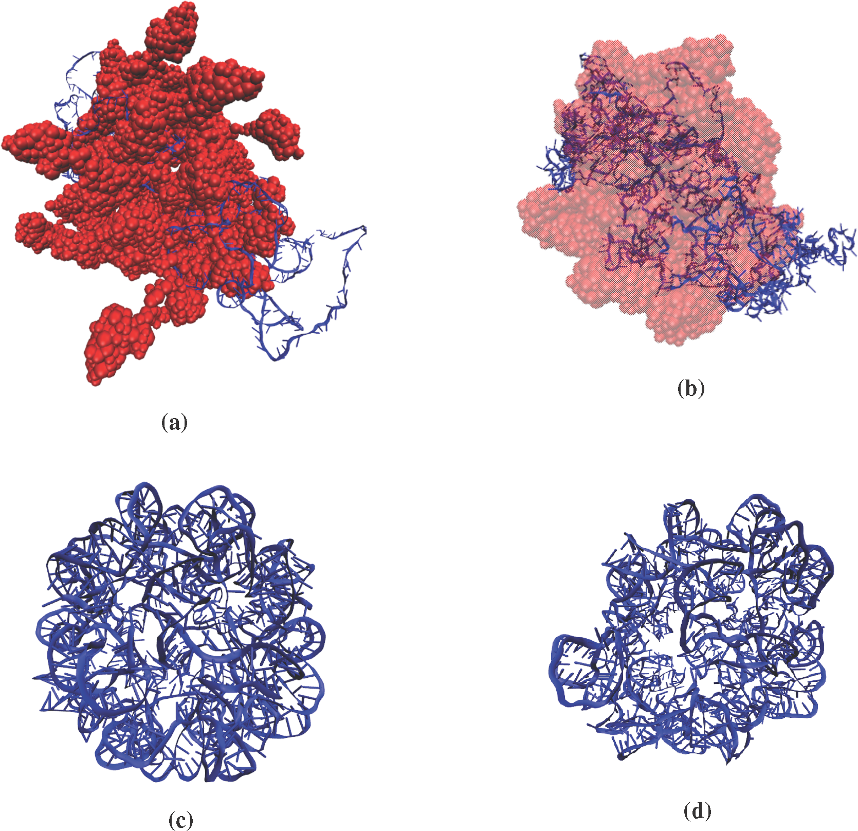
Consider a 10-ns MD simulation of STMV protein monomers assembling with RNA in 0.25 M NaCl (Figure 1). The initial configuration of the system is a random-coil state of the 949 nucleotide RNA surrounded by 60 randomly-placed capsid monomers (accounting for 12 pentamers). During the simulation, proteins are electrostatically attracted to the RNA, and the system begins to organize into an RNA core with an external protein shell. With this, the protein monomers gradually transition from disconnected to a non-covalently bonded state. There exist multiple pathways that lead to such self-assembly in STMV [48]. However, the aim of this study is not to analyze these mechanisms (Figure 2). Here, it is understood how such a structural transition can be captured by the Langevin 
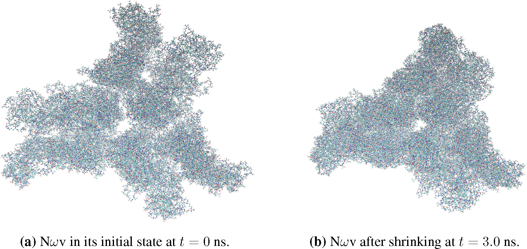
Equations (20). To probe the contributions from different terms in the equations as they vary with the nature of system dynamics, OPs, CMs, thermal forces and diffusions from the MD assembly simulation are compared to those from an RNA expansion in 0.25 M NaCl solution. The RNA of STMV is tightly encased within the capsid core in an icosahedral structure via strong electrostatic interactions [48]. As the capsid is removed, electrostatic repulsion among neighboring negatively-charged nucleotides causes the system to expand, so that the repulsive forces subside [21]. This simulation provides a contrasting example to that of the assembly as, now, the subunits (the pentamers of nucleotide helices (Figure 2)) are moving further apart and not towards one another. Furthermore, the connectivity of the system is maintained throughout the simulation.
In this vein, all-atom configurations derived every 100 ps from the MD simulation of the monomer assembly are used in Equations (2) and (4) to reconstruct the evolution of CMs and global OPs. The OPs considered (with k = {100, 010, 001}) capture the overall dilation/compression of the STMV-RNA assembly along the three Cartesian directions, and R ¯ incorporates the CMs of the protein monomers. The results of MD simulations imply that the rate of change of polynomials U is slower than that of the OPs Φ ¯, which, in turn, is slower than the subsystem CMs R ¯. This is because, while U and Φ ¯ characterize the motion of the entire system, Φ ¯ does so for only a subunit. In particular, the change in the basis functions U is the slowest, as it varies smoothly across the system. Though slow, such changes suggest the use of a dynamical reference configuration for constructing OPs. All three variables, in turn, change on a timescale several orders of magnitude larger than atomic fluctuations. Thus, even though there exists a spatio-temporal scale separation between the three types of coarse-grained variables, it is much smaller in comparison to their separation with the atomic scale. As a result, it is assumed that the three variables change on a similar timescale relative to all-atom fluctuations. Finally, in order to gauge the accuracy of multiscale simulations, their results are benchmarked against those from conventional MD. The RNA-mediated protein assembly and expansion of the capsid-free RNA are simulated for 10 ns. The multiscale and MD simulations are implemented with identical initial structures and conditions from the previous section.
First, consider the results from the assembly simulation. The system is described using 33 global OPs along with 23 subsystem OPs for each of the 60 monomers and 33 variables elucidating the coarse-grained structure of the RNA. The number of these OPs is a natural consequence of the residual minimization within Equation (3) and therefore implies maximum structural information at the CG level. This set of OPs can be systematically enriched if found to be incomplete (
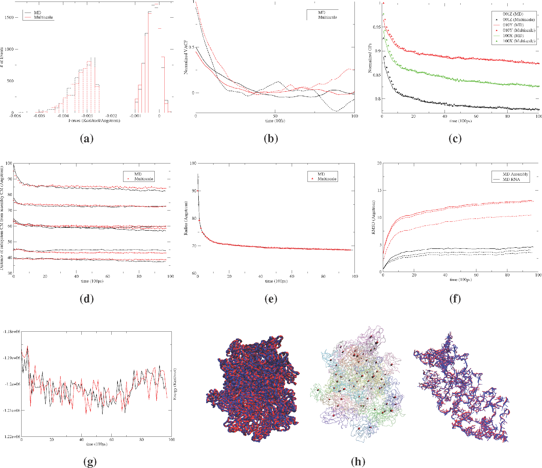
i.e., when the OP velocity autocorrelation functions possess long-time tails. Simulation results imply the global, as well as subsystem thermal averaged force distribution, and the diffusion coefficients show excellent agreement with those from MD (Figures 2a,b). As above, the forces on the monomers are primarily negative, implying attractive interaction with the RNA. Such forces facilitate the observed aggregation. The evolution of large-scale structural variables, including global and subsystem OPs, radius of gyration and root mean square deviation (RMSD) from the initial configuration, are presented in Figures 2c–f. Figure 2g shows the potential energy for the multiscale and MD simulations. These structural variables and energy profiles show excellent agreement in trend, as well as in magnitude. As the protein monomers and the RNA aggregate, the potential energy gradually decreases, indicating stabilization of the system. This trend is consistent with an increase in the number of inter-nucleic acid hydrogen bonds and suggests that the RNA gains a secondary structure during assembly. The observed difference is within the limits of those from multiple MD runs beginning from the same initial structure with different initial velocities. The agreement in simulated trends, as also visually confirmed in Figure 2h, suggests that the multiscale procedure generates configurations consistent with the overall structural changes that arise in MD. However, care should be taken in comparing atomic scale details, such as the dihedral angle or bond length distribution, between the conventional and multiscale simulation procedures. The latter evolves an ensemble of all-atom configurations, e.g., ensembles of size 2 × 10³ generated during every Langevin time step of 50 ps, to compute forces and diffusions. The thermal averaged forces remain practically unchanged with a further increase in ensemble size. Thus, such trajectories should be compared to an average sample of multiple MD (or a single very long MD) simulations. Such MD simulations are infeasible for this system, due to the large number of atoms involved and the long times needed to study the phenomena of interest. Therefore, a strict computational time comparison is avoided, though the equivalence of our multiscale simulations with ensemble MD methods at the atomic scale has been investigated for smaller systems, such as lactoferrin [19,45].
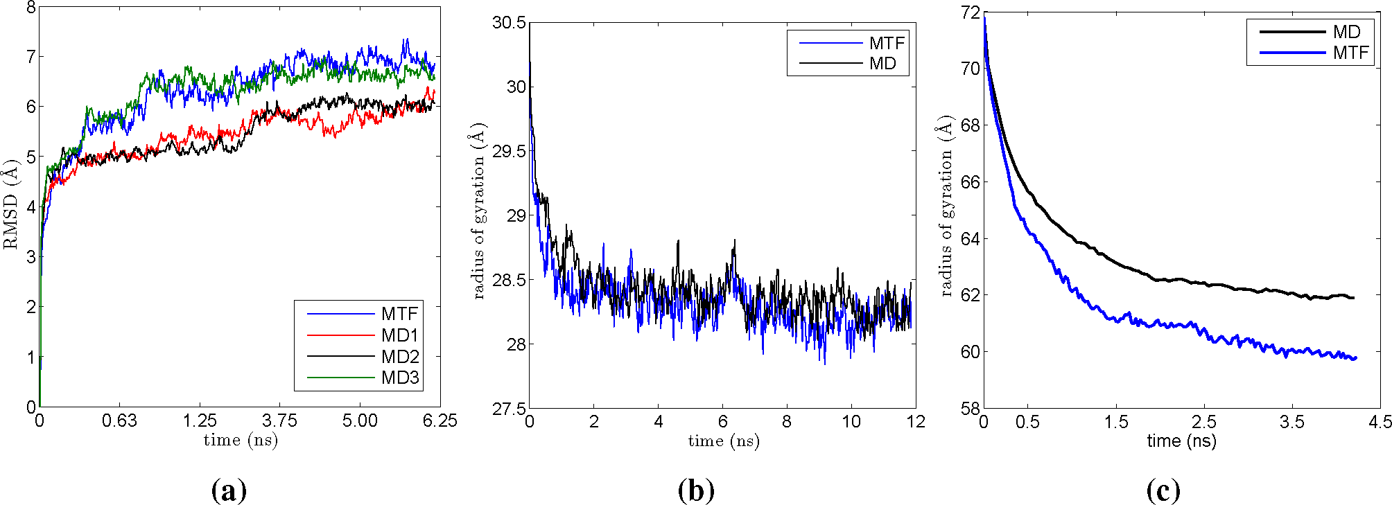
The MD and multiscale trajectories of RNA expansion also show comparable trends. These data are not presented here for the sake of brevity (see [21]). Multiscale trajectories for both of the demonstration systems are repeated using a fixed versus dynamical reference structure. In Figure 2f, the resulting RMSDs from the identical initial structures are presented. For the RNA, the multiscale trajectories with and without re-referencing show considerable agreement with those from MD. Contrastingly, for the protein assembly, only the trajectory with the dynamical reference structure shows agreement with MD. From this result, independent multiscale simulations confirm the need for the coupled evolution of reference configuration CMs, OPs and atomic ensembles to account for complex deformations in macromolecular assemblies. With these results, it is apparent that the multiscale methodology induces an algorithm that can be implemented to simulate the behavior of slowly-evolving phenomena within macromolecular systems at a fraction of the computational expense incurred by the use of long-time MD simulation.

3. Multiscale Factorization

Another recent development is the use of an operator splitting technique to simulate multiscale dynamics. The analytical and computational method discussed within this section, called multiscale factorization, integrates the notions of multiscale analysis, Trotter factorization [49,50] and a stationarity hypothesis, namely that the momenta conjugate to coarse-grained variables can be treated as a stationary random process.
As in the previous section, the first step is to introduce a set of CG variables Φ related to Γ via Φ = Φ ˜ ( Γ ) for a specified function Φ ˜ ( Γ ). When this dependence is well chosen, the CG variables evolve much more slowly than the fluctuations of small subsets of atoms. The N-atom Liouville equation can be solved perturbatively for these CG variables in terms of a smallness parameter ε [21,22,51], a ratio of the characteristic time of the fluctuations of small clusters of atoms to the characteristic time of CG variable evolution. This is achieved by beginning with the ansatz that ρ depends on Γ, both directly and, via Φ ˜, indirectly. The theory proceeds by constructing ρ (Γ, Φ; t) perturbatively in ε as before. To further advance the multiscale approach, the method of Trotter factorization is introduced within the analysis. Using the Trotter factorization scheme within the Liouville operator, the long-time evolution of the system separates into alternating phases of all-atom simulations and CG variable updates. The computational efficiency of the associated numerical method follows from the hypothesis that, should a scale separation truly exist between the atomic and CG variables, the momenta conjugate to the CG variables can be represented as stationary random processes on the atomic timescale. The net result is a computational algorithm with some of the character of the perturbation method and previous approaches [2325,29,30], but with additional control on accuracy, greater efficiency and a more rigorous theoretical basis when such a separation exists. Within this section, the theoretical framework is derived, and simulation methods induced by this approach are discussed and demonstrated for two systems of biological importance—lactoferrin and Nudaurelia capensis omega virus (see Figures 3 and 4) —to assess its accuracy and scaling with the system size.

3.1. Theoretical Formulation

The Newtonian description of an N-atom system is provided by the 6N atomic positions and momenta, collectively denoted by Γ, as in the previous section. The phenomena of interest involve overall transformations of an N-atom system. While Γ contains all of the information needed to solve the problem in principle, it is convenient to introduce a set of CG variables, denoted by Φ, that are used to track the large spatial scale and long-time degrees of freedom, as in Section 2. For example, Φ could describe the overall position, size, shape and orientation of a nanoparticle. As before, a change in Φ involves the coherent deformation of the N-atom system, which implies that the rate of change of Φ is expected to be slow [21,32]. The slowness of these variables directly implies the separation of timescales, which provides a highly-efficient and accurate algorithm for simulating multiscale systems comprised of many atoms.
With this unfolded (Γ, Φ) description, the separated Newtonian dynamics takes the form:
d Γ d t = Γ ,
d Φ d t = Φ ˜ ( Γ ) ,
where the unfolded Liouvillian is decomposed into two operators = Γ + Φ, such that:
Γ = i = 1 N p i m i ( r i ) Φ + f i ( p i ) Φ , Φ = k = 1 N C G Π k ( Φ k ) Γ .
Here, Π k is the CG momentum associated with the kth CG variable and determined explicitly by Π k = Φ ˜ k. The system of Equations (21) and (22) has the formal solution:
( Γ ( t ) , Φ ( t ) ) = S ( t ) ( Γ 0 , Φ 0 )
for initial data Γ0 and Φ0, and the evolution semigroup operator S ( t ) = e t.
By considering the unfolded Liouvillian, the time evolution operator can also be decomposed into the form S ( t ) = e ( Γ + Φ ) t. Since Γ and Φ do not commute, S(t) cannot be factorized into a product of exponential operators. However, Trotter’s theorem [49] can be used to factor the evolution operator as the limit of an ordered product of semigroups using the approximate formula:
S ( t ) [ e Γ t / 2 M e Φ t / M e Γ t / 2 M ] M + O ( ( t M ) 3 )
as M → ∞. By setting t/M to be equal to the discrete time step Δ, the step-wise operator can be expressed as:
S ( Δ ) e Γ Δ / 2 e Φ Δ e Γ Δ / 2 + O ( Δ 3 )
as Δ 0. Let the step-wise semigroup operators S Γ ( t ) = e Γ t and S Φ ( t ) = e Φ tcorrespond to their generating operators, Γ and Φ, respectively. Then, by iterating the stepwise Formula (23), the operator S(nΔ) takes the form:
S ( n Δ ) = i = 1 n S Γ ( Δ 2 ) S Φ ( Δ ) S Γ ( Δ 2 ) .
Using the semigroup property and replacing SΓ(Δ/2) by SΓ(Δ)SΓ(Δ/2) in the second instance of this operator, Equation (24) becomes:
S ( n Δ ) = S Γ ( Δ 2 ) [ i = 1 n S Φ ( Δ ) S Γ ( Δ ) ] S Γ ( Δ 2 ) .
Since the long-time evolution of a multiscale system is the matter of interest, one can neglect the far left and right end terms, SΓ (Δ/2) and SΓ (Δ/2), respectively, to a good approximation. Therefore, for computational purposes, the final step-wise time operator can be defined as:
S ( Δ ) = S Φ ( Δ ) S Γ ( Δ ) .
Next, this factorization is shown to imply a straightforward computational algorithm for solving the dynamical equations for Γ and Φ.

3.2. Computational Implementation and Simulation

One crucial idea that drives the efficiency of the multiscale factorization (MTF) method is the postulate that the momenta conjugate to the CG variables can be represented by a stationary stochastic process over a period of time much shorter than the time scale characteristic of CG evolution. Thus, in a time period significantly shorter than the increment ∆ of the step-wise evolution, the system visits a representative ensemble of configurations consistent with the slowly evolving CG state. This enables one to use an MD simulation for the microscopic phase of the step-wise evolution that is much shorter than Δ to integrate the CG state to the next CG time step. For each of a set of time intervals much less than Δ, the friction-dominated system experiences the same ensemble of conjugate momentum fluctuations. Thus, if δ is the time for which the conjugate momentum undergoes a representative sample of values (i.e., is described by the stationarity hypothesis), then the computational advantage over conventional MD is expected to be approximately Δ.
The two-phase updating suggested by Equation (25) can be achieved for each time-step Δ within simulations as follows. For the SΓ(Δ) phase, conventional MD is used to describe the atomic dynamics. This yields a time-series for Γ and, hence, Π. For all systems simulated in the current study, Π was found to be a stationary random process. Therefore, MD need only be carried out for a fraction of Δ, denoted by δ. This timescale separation and the slowness of the CG variables are the fundamental sources of the computational efficiency of the algorithm. For the SΦ phase updating in the friction dominated regime, the Π time series constructed in the microscopic simulation phase is used to advance Φ in time using the simple, first-order integration scheme:
Φ ( t + Δ ) = Φ ( t ) + t t + Δ Π ( t ) d t .
Due to the stationarity of Π, the integral on the right-hand side reduces drastically and can be strongly approximated by:
t t + Δ Π ( t ) d t Δ δ t t + δ Π ( t ) d t .
Of course, the expression for Π depends on the choice of CG variables. In the current context, the space-warping method [25,26] that maps a set of atomic coordinates to a set of CG variables capturing the coherent deformation of a molecular system in space is utilized. Within this method, the explicit relationship between CG variables and the atomic coordinates is given by:
r i = k ¯ Φ k ¯ U k ¯ i + σ i ,
which is analogous to the relationship between OPs and subsystem CMS of the multiscale perturbation method. Here, k ¯ is a triplet of indices, i is the atomic index, r i is the Cartesian position vector for atom i, Φ k ¯ is a Cartesian vector for CG variable k ¯ and the vector σ i represents the atomic-scale corrections to the coherent deformations generated by Φ k ¯. The basis functions U k ¯ are constructed in two stages. First, they are computed from a product of three Legendre polynomials of order k1, k2 and k3 for the x, y and z dependence, respectively. In the second stage, the basis functions are mass-weighted orthogonalized via a QR decomposition as for the OPs of the multiscale perturbation theory and other studies [21,32]. For instance, the zeroth order polynomial is U 000; the first order polynomial forms a set of three basis functions: U 001, U 010, U 100, and so on. Furthermore, the basis functions depend on a reference configuration r 0, which is updated periodically (once every 10 CG time steps) to control the accuracy. This portion of the OP construction differs greatly from that of the previous section, wherein basis functions depended on slowly-evolving variables and not a reference configuration. Introducing CG variables in this way facilitates the construction of microstates consistent with the CG state [25]. This is achieved by minimizing i = 1 N m i | σ i | 2 with respect to Φ k ¯, as in the previous development. The result is that the CG variables are generalized centers of mass, specifically:
Φ k ¯ = i = 1 N m i U k ¯ i r i i = 1 N m i | U k ¯ i | 2 ,
where mi is the mass of atom i. For the lowest order CG variable, U 000 = 1, and this implies that Φ000 is the center of mass of the system. As the order of the polynomial increases, the CG variables capture more information from the atomic scale, but they vary less slowly with time. Therefore, the space warping CG variables can be classified into low order and high order variables. The former characterizes the larger scale disturbances, while the latter captures short-scale ones [21,32]. Equation (27) then yields a representation for the conjugate momenta:
Π k ¯ = i = 1 N U k ¯ i p i i = 1 N m i | U k ¯ i | 2 ,
where p i is a vector of momenta for the i−th atom. With Φ(t + Δ) computed via Equation (26), the two-phase Δ update is complete, and this cycle is repeated for an arbitrary, but finite, number of discrete time steps. For additional details regarding the necessary energy minimization and equilibration needed for every CG step, we refer the reader to earlier work of the authors [21,29,30]. With this algorithm in place, the final step is to implement a number of trial simulations for relevant demonstration systems.

3.3. Demonstration Systems and Discussion

The two-phase coevolution algorithm presented in this section was implemented using NAMD [46] for the SΓ phase within the framework of the DMS software package [20,21,45]. Numerical computations were performed with the aid of LOOS [52], a lightweight object-oriented structure library. All simulations were performed in vacuum under NVT conditions to assess the scalability and accuracy of the algorithm. The first system used for validation and benchmarking is lactoferrin (LFG). This iron-binding protein is composed of a distal and two proximal lobes (shown in Figure 3a). Two free energy minimizing conformations have been demonstrated experimentally: diferric with closed proximal lobes (PDB Code 1LFG) and apo with open lobes [53] (PDB Code 1LFH). Here, the simulation begins with an open lactoferrin structure and details its closing in a vacuum (see Figure 3). The root mean square deviation (RMSD) for lactoferrin is plotted as a function of time in Figure 5a. This quantity demonstrates that the protein reaches equilibrium in about 5 ns. The transition leads to a decrease in the radius of gyration of the protein by approximately 0.2 nm, as shown in Figure 5b.
The second demonstration system is a triangular structure of the Nudaurelia capensis omega virus (NωV) capsid protein [54] (PDB Code 1OHF) containing three protomers (see Figure 4). Starting from a deprotonated state (at low pH), the system was equilibrated using an implicit solvent. We note that this system is characterized by strong protein-protein interactions. As a result, the virus shrinks in a vacuum after a short period of equilibration, and the computed radius of gyration is shown in Figure 5c.
Based on the convergence of the time integral of Π (see Figure 6), the SΓ phase was chosen to consist of 10 × 104 MD steps for LFG and Nωv, where each MD step is equal to 1 fs. The CG time step, Δ, on the other hand, was taken to be 12.5 ps for LFG and 25 ps for Nωv. Hence, the CG time step is around 104-times that of a single MD time step. Since the MTF algorithm is split into 50% microstate steps, each consisting only of MD simulations, and 50% coarse steps, each consisting of a single CG simulation, the gain in computational efficiency for the multiscale factorization algorithm is on the order of 5 × 10³ in comparison to traditional MD simulation. That is, MTF simulations are around 5000 times faster than traditional MD. Other systems have been simulated using the multiscale factorization algorithm; see [55] for additional details, in particular the computational results concerning the cowpea chlorotic mottle virus (CCMV) full native capsid.
Generally speaking, the multiscale factorization algorithm introduced here can be further optimized to produce greater speedup factors. In particular, the results obtained within the current work can be significantly improved within future studies by incorporating the following changes:
  • After updating the CGs in the two-phase coevolution Trotter cycle, it is necessary to fine grain, i.e., develop the atomistic configuration to be used as an input to MD. Recently, it has been discovered that the CPU time to achieve this fine graining can be dramatically reduced via a constraint method that eliminates bond length and angle strains.
  • Information from earlier steps in the discrete time evolution can be used to increase the CG time step and achieve greater numerical stability. While this was demonstrated for one multiscale algorithm [45], it can also be adapted to and further developed for the current multiscale factorization method.
  • The time stepping algorithm used in this work is the analogue of the first-order Euler method for ordinary differential equations. Hence, greater numerical stability and efficiency could be achieved for a system of stiff differential equations using standard implicit and semi-implicit schemes [56], rather than the basic numerical integrator chosen here.

4. Conclusions

The present study discusses two recent multiscale methods, which stem from an N-atom formulation and can be used to study multiscale systems in a friction-dominated regime. The first, the multiscale perturbation theory, provides a self-consistent theory of macromolecular assembly, wherein a set of equations is derived to describe the coupled stochastic dynamics of OPs and molecules. It also introduces an algorithm to co-evolve OPs and individual molecules over long periods of time, so as to enable a calibration-free framework. More precisely, the set of OPs and the associated multiscale algorithm incorporate the hierarchical nature of the assembly architecture. Overall subsystem deformations, like extension, compression, rotation and translation, as well as resulting inter-system motions that probe the temporal dynamics of the assembly are accounted for within the formulation. In addition, rapid motions, such as internal subsystem dynamics or high frequency fluctuations can be probed via a quasi-equilibrium ensemble of all-atom configurations. Unlike MD, in which time steps are limited to 1014 seconds or less, the perturbation method allows time steps that are many orders of magnitude greater. While a computational difficulty arises from the construction of the thermal average forces and diffusion factors, the associated CPU time is more than offset by the large Langevin time steps. This force-field-based methodology takes advantage of the structural hierarchy natural to macromolecular assemblies in defining the system as a collection of mutually interacting subsystems with internal dynamics, which simultaneously preserves the all-atom description.
The second multiscale method, multiscale factorization, was described and implemented within Section 3 and introduces the additional benefits of a multiscale theory of the Liouville equation by incorporating Trotter factorization and the stationary hypothesis for variables conjugate to the CG description. A key advantage is that this approach avoids the need for the resource-consuming diffusion factors, thermal average and random forces necessary to utilize the multiscale perturbation approach. That being said, the CG variables for the mesoscopic systems of interest do possess a degree of stochastic behavior. In the present formulation, this stochasticity is accounted for via a series of MD steps used in the phase of the multiscale factorization algorithm, wherein the N-atom probability density is evolved via Γ, i.e., at the constant value of the CG variables.
Both methods provide a rigorous mathematical framework, a self-consistent theory and multiscale computational algorithms for accurately and efficiently simulating a wide variety of physical and biological phenomena over long times, as demonstrated for multiple scale systems, like STMV, lactoferrin and NωV. However, each method is better suited to distinct physical or biological systems that possess unique characteristics. In particular, the multiscale perturbation method requires a separation of (in this case, mass) scales in order to be applicable and enable fast computations. Memory effects within the system of interest are then incorporated into the stochastic nature of the associated Langevin equations. In contrast, the multiscale factorization method does not require an explicitly-defined scale separation in order to remain valid. Instead, a stationarity hypothesis on the CG momenta is utilized to enable efficient simulations without the need for the Langevin description or the computation of expensive parameters, such as diffusion coefficients and thermal averaged forces. Additionally, the stochasticity in the system appears within a series of MD steps utilized by the multiscale algorithm rather than a Langevin step. Within the latter method, however, the stationarity assumption must be a priori verified, and for some rapidly-evolving physical systems, this may not possible. Hence, each method can be quite useful and drastically reduce the computational resources necessary to simulate multiscale phenomena, but the system features needed to implement each method may differ dramatically. An attempt to unify these two methods seems unlikely, but this is the subject of ongoing research.
Regardless of their subtle differences, the development of these multiscale methods is crucial to advance the scientific state-of-the-art, as traditional computational tools, like MD, cannot simulate such large systems over long time periods in a feasible amount of computational time. As both of the methods presented herein achieve a sizable gain in efficiency while maintaining a demonstrably highly level of accuracy, they represent important advances in the computation of macromolecular assemblies.

Acknowledgments

The authors appreciate and acknowledge the support of the NSF INSPIRE program, the NSF Division of Mathematical Sciences (under Grants DMS-0908413 and DMS-1211667), NIH and Indiana University’s College of Arts and Sciences.

Author Contributions

S.P. and P.O. conceived and designed the computational experiments; S.P. performed the computational experiments; S.P. and P.O. analyzed the data; S.P. wrote the paper.

Conflicts of Interest

The authors declare no conflict of interest.

References

  1. Wegst, U.; Ashby, M. The mechanical efficiency of natural materials. Philos. Mag. 2004, 84, 2167–2181. [Google Scholar]
  2. Meyers, M.; Chen, P.; Lin, A.; Seki, Y. Biological materials: Structure and mechanical properties. Prog. Mat. Sci. 2008, 53, 1–206. [Google Scholar]
  3. Yin, Y.; Arkhipov, A.; Schulten, K. Simulations of membrane tubulation by lattices of amphiphysin N-BAR domain. Structure 2009, 17, 882–892. [Google Scholar]
  4. Limbach, H.; Arnold, A.; Mann, B.; Holm, C. ESPResSo—An extensible simulation package for research on soft matter systems. Comput. Phys. Commun. 2006, 174, 704–727. [Google Scholar]
  5. Abraham, F.; Walkup, R.; Gao, H.; Duchaineau, M.; de la Rubia, T.D.; Seager, M. Simulating materials failure by using up to one billion atoms and the world’s fastest computer: Brittle fracture. Proc. Natl. Acad. Sci. USA 2002, 99, 5777–5782. [Google Scholar]
  6. Schulz, R.; Lindner, B.; Petridis, L.; Smith, J. Scaling of Multimillion-Atom Biological Molecular Dynamics Simulation on a Petascale Computer. J. Chem. Theor. Comput. 2009, 5, 2798–2808. [Google Scholar]
  7. Uvarov, A.; Fritzsche, S. Friction of N-bead macromolecules in solution: Effects of the bead-solvent interaction. Phys. Rev. E 2006, 73, 011111. [Google Scholar]
  8. Chao, S.; Kress, J.; Redondo, A. Coarse-grained rigid blob model for soft matter simulations. J. Chem. Phys. 2005, 122, 234912. [Google Scholar]
  9. Arkhipov, A.; Freddolino, A.; Schulten, K. Stability and dynamics of virus capsids described by coarse-grained modeling. Structure 2006, 14, 1767–1777. [Google Scholar]
  10. Gohlke, H.; Thorpe, M. A Natural Coarse Graining for Simulating Large Biomolecular Motion. Biophys. J 2006, 91, 2115–2120. [Google Scholar]
  11. Backofen, R.; Maher, M.; Puget, J. Constraint Techniques for Solving the Protein Structure Prediction Problem; Principles and Practice of Constraint Programming—CP98; Springer: Berlin/Heidelberg, Germany, 1998. [Google Scholar]
  12. Shreif, Z.; Ortoleva, P. Curvilinear All-Atom Multiscale (CAM) Theory of Macromolecular Dynamics. J. Stat. Phys. 2008, 130, 669–685. [Google Scholar]
  13. Amadei, A.; Linssen, A.; Berendsen, H. Essential dynamics of proteins. Proteins Struct. Funct. Bioinform. 1993, 17, 412–425. [Google Scholar]
  14. Hayward, S.; Kitao, A.; Go, N. Harmonicity and anharmonicity in protein dynamics: A normal mode analysis and principal component analysis. Proteins Struct. Funct. Bioinform. 1995, 23, 177–186. [Google Scholar]
  15. Lyubartsev, A.; Karttunen, M.; Vattulainen, I.; Laaksonen, A. On coarse-graining by the inverse monte carlo method: Dissipative particle dynamics simulations made to a precise tool in soft matter modeling. Soft Mater. 2002, 1, 121–137. [Google Scholar]
  16. Murtola, T.; Bunker, A.; Vattulainen, I.; Deserno, M.; Karttunen, M. Multiscale modeling of emergent materials: Biological and soft matter. Phys. Chem. Chem. Phys. 2009, 11, 1869–1892. [Google Scholar]
  17. Joshi, H.; Singharoy, A.; Sereda, Y.; Cheluvaraja, S.; Ortoleva, P. Multiscale simulation of microbe structure and dynamics. Prog. Biophys. Mol. Biol. 2011, 107, 200–217. [Google Scholar]
  18. Praprotnik, M.; Delle Site, L.; Kremer, K. Multiscale simulation of soft matter: From scale bridging to adaptive resolution. Ann. Rev. Phys. Chem. 2008, 59, 545–571. [Google Scholar]
  19. Ortoleva, P.; Singharoy, A.; Pankavich, S. Hierarchical Multiscale Modeling of Macromolecules and Their Assemblies. Soft Matter. 2013, 9, 4319–4335. [Google Scholar]
  20. Cheluvaraja, S.; Ortoleva, P.J. Thermal Nanostructure: An Order Parameter/Multiscale Ensemble Approach. J. Chem. Phys. 2010, 132, 75102–75110. [Google Scholar]
  21. Singharoy, A.; Cheluvaraja, S.; Ortoleva, P.J. Order Parameters for Macromolecules: Application to Multiscale Simulations. J. Chem. Phys. 2011, 134, 44104–44120. [Google Scholar]
  22. Ortoleva, P.J. Nanoparticle Dynamics: A Multiscale Analysis of the Liouville Equation. J. Phys. Chem. B 2005, 109, 21258–21266. [Google Scholar]
  23. Pankavich, S.; Shreif, Z.; Ortoleva, P.J. Multiscaling for Classical Nanosystems: Derivation of Smoluchowski and Fokker-Planck Equations. Phys. A 2008, 387, 4053–4069. [Google Scholar]
  24. Pankavich, S.; Shreif, Z.; Miao, Y.; Ortoleva, P.J. Self-Assembly of Nanocomponents into Composite Structures: Derivation and Simulation of Langevin Equations. J. Chem. Phys. 2009, 130, 194115–194124. [Google Scholar]
  25. Pankavich, S.; Miao, Y.; Ortoleva, J.; Shreif, Z.; Ortoleva, P. Stochastic Dynamics of Bionanosystems: Multiscale Analysis and Specialized Ensembles. J. Chem. Phys. 2008, 128, 234908. [Google Scholar]
  26. Jaqaman, K.; Ortoleva, P.J. New space warping method for the simulation of large-scale macromolecular conformational changes. J. Comput. Chem. 2002, 23, 484–491. [Google Scholar]
  27. Shreif, Z.; Pankavich, S.; Ortoleva, P. Liquid-crystal transitions: A first-principles multiscale approach. Phys. Rev. E 2009, 80, 031703. [Google Scholar]
  28. Pankavich, S.; Shrief, Z.; Chen, Y.; Ortoleva, P. Multiscale Theory of Boson Droplets: Implications for Collective and Single-Particle Excitations. Phys. Rev. A 2009, 79, 013628. [Google Scholar]
  29. Miao, Y.; Ortoleva, P. Molecular Dynamics/Order Parameter EXtrapolation (MD/OPX) for Bionanosystem Simulations. J. Comput. Chem. 2008, 30, 423–437. [Google Scholar]
  30. Miao, Y.; Johnson, J.E.; Ortoleva, P.J. All-Atom Multiscale Simulation of Cowpea Chlorotic Mottle Virus Capsid Swelling. J. Phys. Chem. B 2010, 114, 11181–11195. [Google Scholar]
  31. Pankavich, S.; Ortoleva, P. Nanosystem Self-Assembly Pathways Discovered via All-Atom Multiscale Analysis. J. Phys. Chem. B 2012, 116, 8355–8362. [Google Scholar]
  32. Singharoy, A.; Joshi, H.; Miao, Y.; Ortoleva, P. Space Warping Order Parameters and Symmetry: Application to Multiscale Simulation of Macromolecular Assemblies. J. Phys. Chem. B 2012, 116, 8423–8434. [Google Scholar]
  33. Chandrasekhar, S. Dynamical Friction. I. General Considerations: The Coefficient of Dynamical Friction. Astrophys. J 1943, 97, 255. [Google Scholar]
  34. Deutch, J.; Oppenheim, I. The Lennard-Jones Lecture. The concept of Brownian motion in modern statistical mechanics. Faraday Discuss. Chem. Soc. Lond. 1987, 83, 1–20. [Google Scholar]
  35. Deutch, J.; Hudson, S.; Ortoleva, P.; Ross, J. Light scattering from systems with chemical oscillations and dissipative structures. J. Chem. Phys. 1972, 57, 4327–4332. [Google Scholar]
  36. Shea, J.-E.; Oppenheim, I. Fokker–Planck Equation and Langevin Equation for One Brownian Particle in a Nonequilibrium Bath. J. Phys. Chem. 1996, 100, 19035–19042. [Google Scholar]
  37. Shea, J.-E.; Oppenheim, I. Fokker–Planck equation and non-linear hydrodynamic equations of a system of several Brownian particles in a non-equilibrium bath. Phys. A 1997, 247, 417–443. [Google Scholar]
  38. Peters, M. Fokker–Planck Equation, Molecular Friction, and Molecular Dynamics for Brownian Particle Transport near External Solid Surfaces. J. Stat. Phys. 1999, 94, 557–587. [Google Scholar]
  39. Peters, M. Fokker–Planck Equation and the Grand Molecular Friction Tensor for Coupled Rotational and Translational Motions of Structured Brownian Particles near Structured Surfaces. J. Chem. Phys. 1999, 110, 528–538. [Google Scholar]
  40. Ma, S.K. Modern Theory of Critical Phenomena (Frontiers in Physics); Benjamin: Reading, MA, USA, 1976. [Google Scholar]
  41. Whitelam, S.; Feng, E.; Hagan, M.; Geissler, P. The role of collective motion in examples of coarsening and self-assembly. Soft Matter. 2009, 5, 1251. [Google Scholar]
  42. Pankavich, S.; Ortoleva, P. Multiscaling for Systems with a Broad Continuum of Characteristic of Lengths and Times: Structural Transitions in Nanocomposites. J. Math. Phys. 2010, 51, 063303. [Google Scholar]
  43. Shreif, Z.; Adhangale, P.; Cheluvaraja, S.; Perera, R.; Kuhn, R.; Ortoleva, P. Enveloped Viruses Understood via Multiscale Simulation: Computer-Aided Vaccine Design. In Scientific Modeling and Simulations; Yip, S., de la Rubia, T.D., Eds.; Lecture Notes in Computational Science and Engineering; Springer Netherlands: Dordrecht, The Netherlands, 2008; pp. 363–380. [Google Scholar]
  44. Singharoy, A.; Sereda, Y.; Ortoleva, P. Hierarchical Order Parameters for Macromolecular Assembly Simulations: Construction and Dynamical Properties of Order Parameters. J. Chem. Theor. Comput. 2012, 8, 1379–1392. [Google Scholar]
  45. Singharoy, A.; Joshi, H.; Ortoleva, P. Multiscale Macromolecular Simulation: Role of Evolving Ensembles. J. Chem. Inf. Model. 2012, 52, 2638–2649. [Google Scholar]
  46. Phillips, J.C.; Braun, R.; Wang, W.; Gumbart, J.; Tajkhorshid, E.; Villa, E.; Chipot, C.; Skeel, R.D.; Kale, L.; Schulten, K. Scalable molecular dynamics with NAMD. J. Comput. Chem. 2005, 26, 1781–1802. [Google Scholar]
  47. Brooks, B.; Brooks, C.; Mackerell, A.; Nilsson, L.; Petrella, R.; Roux, B.; Won, Y.; Archontis, G.; Bartels, C.; Caflisch, S.; et al. CHARMM: The biomolecular simulation program. J. Comput. Chem. 2009, 30, 1545–1614. [Google Scholar]
  48. Schneemann, A. The Structural and Functional Role of RNA in Icosahedral Virus Assembly. Annu. Rev. Microbiol. 2006, 60, 51–67. [Google Scholar]
  49. Trotter, H.F. On the product of semi-groups of operators. Proc. Am. Math. Soc. 1959, 10, 545–551. [Google Scholar]
  50. Tuckerman, M.; Berne, B.J.; Martyna, G.J. Reversible multiple time scale molecular dynamics. J. Chem. Phys. 1992, 97, 1990–2001. [Google Scholar]
  51. Joshi, H.; Singharoy, A.; Sereda, Y.V.; Cheluvaraja, S.C.; Ortoleva, P. Multiscale simulation of microbe structure and dynamics. Prog. Biophys. Mol. Biol. 2011, 107, 200–217. [Google Scholar]
  52. Romo, T.; Grossfield, A. LOOS: An Extensible Platform for the Structural Analysis of Simulations, Proceedings of the 31st Annual International Conference of the IEEE EMBS, Minneapolis, MN, USA, 2–6 September 2009; pp. 2332–2335.
  53. Norris, G.E.; Anderson, B.F.; Baker, E.N. Molecular replacement solution of the structure of apolactoferrin, a protein displaying large-scale conformational change. Acta Crystallogr. Sect. B 1991, 47, 998–1004. [Google Scholar]
  54. Taylor, D.J.; Wang, Q.; Bothner, B.; Natarajan, P.; Finn, M.G.; Johnson, J.E. Correlation of chemical reactivity of nudaurelia capensis ω virus with a pH-induced conformational change. J. Chem. Commun. 2003, 22, 2770–2771. [Google Scholar]
  55. Abi Mansour, A.; Ortoleva, P. Multiscale Factorization Method for Simulating Mesoscopic Systems with Atomic Precision. J. Chem. Theory Comput. 2014, 10, 518–523. [Google Scholar]
  56. LeVeque, R. Finite Difference Methods for Ordinary and Partial Differential Equations: Steady-State and Time-Dependent Problems; Society for Industrial and Applied Mathematics (SIAM): Philadelphia, PA, USA, 2007. [Google Scholar]
Figure 1. (a) Initial (0 ns) and (b) final (10 ns) structures of the STMV protein monomers aggregating with RNA; (c,d) same as (a) and (b), respectively, but for the expansion of free RNA in aqueous solution. These simulations are chosen to illustrate two contrasting scenarios of inter-subsystem interaction and their effect on the Langevin dynamics of the order parameters (OPs). The random coil structure of the RNA in (a) is generated using the ROSETTA molecular modeling software package, and the icosahedral symmetric form is extracted from its encapsidated state, as also used in [9].
Computation 03 00029f1
Figure 2. Distributions of the typical (a) subsystem center of mass (CM) (dotted) and OP (Φ100X) (solid) forces; and (b) the associated velocity autocorrelation functions from 10 ns MD and multiscale simulations of the satellite tobacco mosaic virus (STMV) protein-RNA assembly; (c) evolution of large-scale structural variables, including: global OPs, (d) subsystem CMs, (e) the radius of gyration and (f) the RMSD from the initial configuration. All numerical results show excellent agreement between MD and multiscale predictions. The RMSD from the initial structure also shows that the Langevin assembly simulation requires referencing to reproduce the MD results; however, capturing the RNA expansion does not require a dynamical reference structure. The dashed line implies the use of a dynamical reference structure, whereas dash-dots imply a fixed reference structure during the Langevin evolution of the system. (g) The potential energy profiles for the multiscale and MD simulations also show strong agreement; (h) visual comparison of multiscale (blue) and MD (red) generated all-atom structures of the assembled monomers and the RNA. Also provided are the positions of subsystem CMs in bead representation (multiscale (black) and MD (red)) showing almost identical configurations.
Computation 03 00029f2
Figure 3. Snapshots of lactoferrin protein in its open (a) and closed (b) states.
Computation 03 00029f3
Figure 4. Snapshots of the Nudaurelia capensis omega virus (NωV) triangular structure before (a) and after (b) contraction due to strong protein-protein interactions.
Computation 03 00029f4
Figure 5. MD and multiscale factorization (MTF) results for lactoferrin and Nωv simulations. (a) RMSD variation of lactoferrin as a function of time for a series of three MD and one MTF runs; (b) the radius of gyration decreases in time as lactoferrin shrinks; (c) temporal evolution of the radius of gyration of Nωv computed using MD and MTF.
Computation 03 00029f5
Figure 6. Evidence for the validity of the stationarity hypothesis shown via the convergence of 1 1 δ 0 δ Π ( t ) d t as a function of δ for coarse-grained (CG) variables selected from among those used in simulating the contraction of Nωv. Initially, the integral experiences large fluctuations, since for δ small, only relatively few configurations are included in the time average constituting the integral, but as δ increases, the statistics improve and the integral becomes increasingly flat. (a) A plot of the time integral of Π for a high order CG Φ200; (b) a plot of the time integral of Π for a low order CG Φ001.
Computation 03 00029f6
Table 1. Input parameters for NAMD (NAnoscale Molecular Dynamics) simulations.
ParameterValues
Temperature300 K
Langevin damping5
Timestep1 fs
FullElectFrequency2 fs
nonbondedFreq1 fs
Box size160 Å × 160 Å 160 Å a
250 Å × 250 Å × 250 Å b
Force-field parameterpar_all27_prot_na.prm
1–4scaling1.0
Switchdist10.0 Å
Cutoff12.0 Å
Pairlistdist20.0 Å
Stepspercycle2
Rigid bondWater
aRNA expansion;
bprotein-RNA assembly.

