Steady-State Anderson Accelerated Coupling of Lattice Boltzmann and Navier–Stokes Solvers

Abstract

We present an Anderson acceleration-based approach to spatially couple three-dimensional Lattice Boltzmann and Navier–Stokes (LBNS) flow simulations. This allows to locally exploit the computational features of both fluid flow solver approaches to the fullest extent and yields enhanced control to match the LB and NS degrees of freedom within the LBNS overlap layer. Designed for parallel Schwarz coupling, the Anderson acceleration allows for the simultaneous execution of both Lattice Boltzmann and Navier–Stokes solver. We detail our coupling methodology, validate it, and study convergence and accuracy of the Anderson accelerated coupling, considering three steady-state scenarios: plane channel flow, flow around a sphere and channel flow across a porous structure. We find that the Anderson accelerated coupling yields a speed-up (in terms of iteration steps) of up to 40% in the considered scenarios, compared to strictly sequential Schwarz coupling.

1. Introduction

The choice of an optimal numerical solver for a given fluid dynamics problem is often problematic. Memory and runtime requirements, numerical accuracy and stability, treatment of boundaries, parallel scalability and flow physics are only some of the criteria that need to be taken into consideration. In particular, many flow problems cannot be grouped into a particular solver’s “favorite problems”. One approach to locally exploit the features of different solvers consists in splitting the computational domain and apply different flow solvers on the respective subdomains.

Navier–Stokes (NS) solvers [1,2] and Lattice Boltzmann (LB) methods [3,4] are well established techniques for simulating in- or weakly compressible fluid flow. One or the other method may be advantageous in particular flow scenarios, and both approaches have been compared [5,6] and studied in detail over the last decades. Moreover, it is well-known that Lattice Boltzmann methods yield the Navier–Stokes equations in the asymptotics of a vanishing Mach number (convective scaling), and even result in the incompressibleNavier–Stokes system using diffusive scaling [7]. They can be considered equivalent in that sense. When using the term “Navier–Stokes solver” in the following, we refer to a direct discretization of the (incompressible) Navier–Stokes system and a respective numerical method solving the arising non-linear system. Despite their particular features—high locality (LB), local/simple treatment of complex geometries (LB), low memory requirements (NS), to only name a few—only little effort has been undertaken so far to spatially couple the two approaches [8,9,10,11,12] or, more generally speaking, to couple LB and direct PDE solvers [13,14].

In [10,11], we developed a coupling methodology and applied it to steady-state and recently to transient problems [15]. In the transient case, we considered explicit coupling of a Lattice Boltzmann and an incompressible Navier–Stokes solver. Although good agreement of the velocity profiles could be obtained in various scenarios, we also demonstrated that minor density/pressure perturbations may have an essential impact on the solution. In order to improve the matching of degrees of freedom at the coupling interface between LB and NS subdomains, more enhanced or pressure correction schemes may represent promising approaches. In this contribution, we take a step towards sophisticated coupling of LB and NS based on overlapping Schwarz-based domain decomposition. We restrict considerations to three-dimensional, steady-state scenarios. We discuss three coupling methodologies—referred to as sequential coupling, parallel coupling and Anderson accelerated coupling, cf. Section 2.3—and study their convergence behavior for channel flow scenarios. A particular focus is put on the Anderson acceleration method. This method has been used to accelerate and stabilize fixed-point iterations in, for example, fluid-structure interaction [16], groundwater flow [17] or electronic structure computations [18]. It dates back to 1965 [19], and recently re-attracted interest as it shows great potential for applications in which a Newton matrix is inaccessible or too expensive to store [20,21]. Though the method requires additional computations for processing the coupled variables at the interface, it has become attractive for HPC simulations as it allows for fully parallel execution of two coupled solvers. Schwarz methods for steady-state coupled problems may require many iterations to converge; the Anderson acceleration technique reduces the number of iterations steps. We demonstrate that these features of the Anderson acceleration also hold for LBNS coupling. We further show that our hybrid LBNS method can be used to efficiently solve flow problems with complex geometries, such as the flow through and around porous media. In particular, both LB and NS can be combined to optimally exploit LB and NS features, that is to reduce memory footprint (NS) while applying the local LB algorithm only in selected regions of interest on a potentially refined grid. This is similar to the idea of LB grid refinement; yet, this approach does not only refine the resolution, but also the model for the fluid flow by combining mesoscopic (LB) and continuum (NS) approaches. Besides, capturing different flow physics by using an efficient LBNS coupling may be enabled. For example, the mesoscopic nature of LB allows to access finite Knudsen flows for regimes up to $\mathrm{Kn}\sim O\left(1\right)$ [22,23], potentially using higher-order LB velocity space discretizations. Flows in micro-devices such as microfluidic networks may thus be simulated using a NS solver in wider bulk regions and a LB solver in narrow regions. Another mesoscopic feature of LB consists in the strictly local treatment of Brownian fluctuations [24] which is basically impossible in the (incompressible) NS context.

We start with a short introduction to LB and NS solvers and a description of the three coupling methods in Section 2. Implementation of the coupling, validation results and a numerical convergence study of the Anderson acceleration scheme are provided in Section 3. We close with a brief conclusion and give an outlook to future work in Section 4.

2. Materials and Methods

2.1. Navier–Stokes

We solve the three-dimensional incompressible Navier–Stokes equations

$$\begin{array}{ccc}\hfill \nabla ·\mathbf{u}& =& 0\hfill \end{array}$$

(1)

$$\begin{array}{ccc}\hfill {\partial }_t\mathbf{u}+(\mathbf{u}·\nabla )\mathbf{u}& =& -\nabla p+\nu \Delta \mathbf{u}\hfill \end{array}$$

(2)

with fluid velocity $\mathbf{u}\in {\mathbb{R}}^3$, pressure $p\in \mathbb{R}$ and kinematic viscosity $\nu \in {\mathbb{R}}^{+}$. We apply the finite difference methodology described in [25]. The computational domain is discretized using a Cartesian grid. The unknowns for pressure and fluid velocity are stored according to a staggered scheme: the pressure is evaluated in the cell centers whereas the velocity components $\mathbf{u}=(u_0,u_1,u_2)$ are computed in the midpoints of the cell faces. A mix of first- and second-order finite differences is employed to discretize the differential expressions in Equations (1) and (2); the first-order expressions are used to enhance stability due to the convection term. An explicit time stepping for the velocities and making use of the continuity Equation (1) results in a Poisson equation for the pressure to be solved in each time step. The complete method is outlined in Algorithm 1.

Algorithm 1 Navier–Stokes time stepping scheme

while $t_n<t_{end}$ do    set boundary conditions    assemble right hand side of Poisson equation    solve Poisson equation ($\to p^{n+1}$)    do time step for velocities ($\to {\mathbf{u}}^{n+1}$)    $n\leftarrow n+1$  end while

2.2. Lattice Boltzmann

We consider the Bhatnagar-Gross-Krook (BGK)-based [26] Lattice Boltzmann method which computes the particle distributions $f_i(\mathbf{x},t)$ according to the well-known “collide-stream” scheme:

$$f_i(\mathbf{x}+{\mathbf{c}}_{i}dt,t+dt)=f_i(\mathbf{x},t)-\frac{1}{\tau }\left(f_i(\mathbf{x},t)-f_i^{eq}(\rho (\mathbf{x},t),\mathbf{u}(\mathbf{x},t))\right),i=1,...,Q.$$

(3)

Fluid density $\rho \in \mathbb{R}$, pressure $p\in \mathbb{R}$, momentum $\rho \mathbf{u}\in {\mathbb{R}}^3$ and equilibrium distributions $f_i^{eq}$ are given by

$$\begin{array}{ccc}\hfill \rho (\mathbf{x},t)& =& \sum _{i=1}^Q{f}_i(\mathbf{x},t)\hfill \end{array}$$

(4)

$$\begin{array}{ccc}\hfill p(\mathbf{x},t)& =& c_s^2\rho (\mathbf{x},t)\hfill \end{array}$$

(5)

$$\begin{array}{ccc}\hfill \rho \mathbf{u}(\mathbf{x},t)& =& \sum _{i=1}^Q{f}_i{\mathbf{c}}_i\hfill \end{array}$$

(6)

$$\begin{array}{ccc}\hfill f_i^{eq}(\rho ,\mathbf{u})& =& w_i\rho \left(1+\frac{{\mathbf{c}}_i\mathbf{u}}{c_s^2}+\frac{{\left({\mathbf{c}}_i\mathbf{u}\right)}^2}{2c_s^4}-\frac{{\mathbf{u}}^2}{2c_s^2}\right)\hfill \end{array}$$

(7)

where $c_s:=1/\sqrt{3}$ and $w_i$ are lattice-specific weights. We consider the discretizations D3Q15, D3Q19 and D3Q27, i.e., $Q\in \{15,19,27\}$. The relaxation time τ is related to the kinematic viscosity of the fluid via $\nu =c_s^2(\tau -0.5)$ and is restricted to the interval $(0.5,2)$ due to stability. It can be shown that the presented Lattice Boltzmann scheme is asymptotically equivalent to solving the Navier–Stokes equations in the weakly compressible limit [27].

2.3. Coupling Strategies

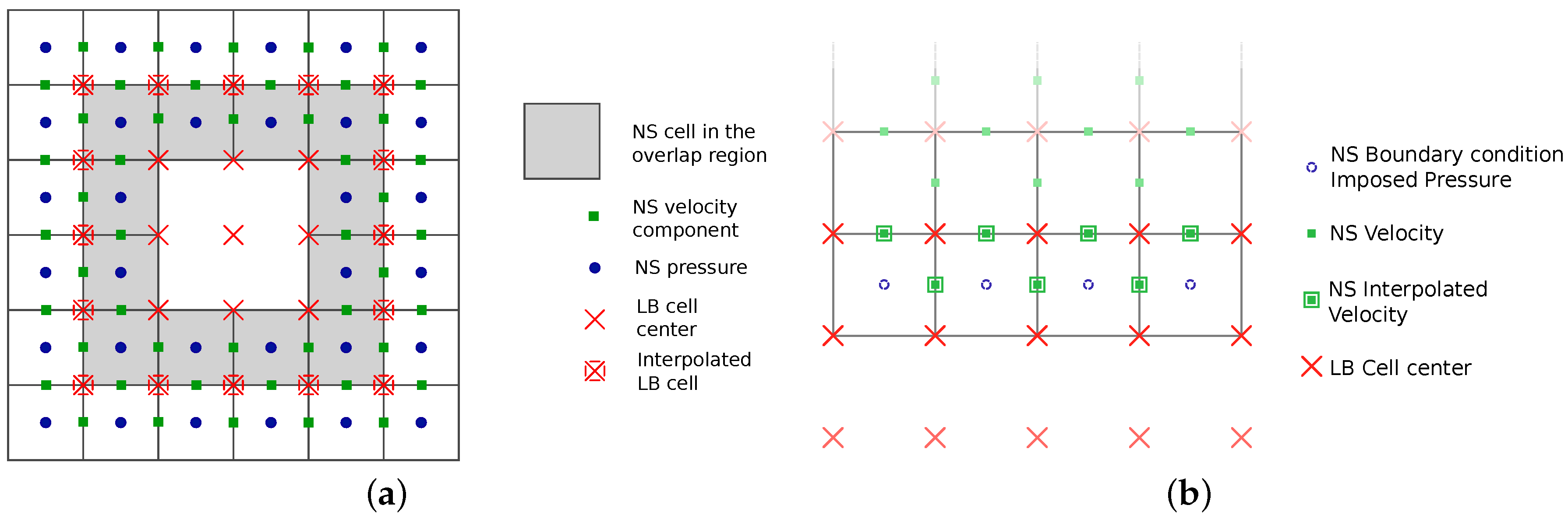
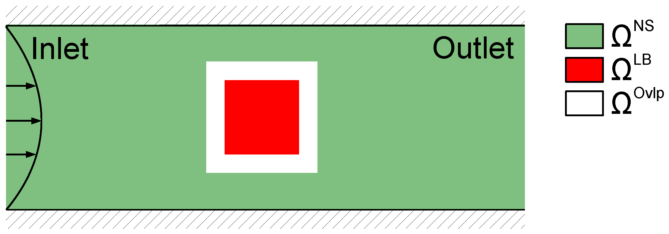
2.3.1. Spatial Coupling: General Methodology

Domain Decomposition, Interpolation and Unit Conversion

We decompose the computational domain into a LB and NS domain. Both domains overlap, see Figure 1; with LB and NS solver operating on Cartesian grids of mesh size $d{x}^{LB}$, $d{x}^{NS}$, the thickness of the overlap region is chosen as $d{x}^{ovlp}:=k·max\{d{x}^{LB},d{x}^{NS}\}$, $k\in \mathbb{N}$, $k\ge 1$.

We have found that the size of the overlap region is a rather insensitive parameter in the coupling. Only for $k=1$, minor deficiencies in the overall accuracy and coupling convergence could be observed. In all our studies, we choose $k=2$ as compromise between minimizing the overlap region on the one hand and tightly coupling flow information of both solvers on the other hand. We expect the application of Cartesian grids—in particular on NS side—to be no strict requirement. Different grids and solvers (such as finite volume or finite element schemes) may be used, and (the thickness of) the overlap region needs to be adapted correspondingly.

We construct valid information on the outer overlap boundary cells of LB/NS using second-order interpolation, applied to the NS/LB quantities, see Figure 2.

Since NS and LB solver work at different units, velocity and pressure values as well as kinematic viscosity need to be matched. Given a kinematic viscosity ν, characteristic velocity $u_c$ and pressure $p_c$ on NS side, LB values are computed as follows:

$$\begin{array}{ccc}\hfill {\nu }^{LB}& =& \nu ·\frac{d{t}^{LB}}{d{x}^{L{B}^2}}\hfill \\ \hfill u_c^{LB}& =& u_c·\frac{d{t}^{LB}}{d{x}^{LB}}\hfill \\ \hfill p_c^{LB}& =& p_c·\frac{d{t}^{L{B}^2}}{d{x}^{L{B}^2}}\hfill \end{array}$$

(8)

where $d{x}^{LB}$, $d{t}^{LB}$ correspond to LB mesh size and time step.

From Lattice Boltzmann to Navier–Stokes

Dirichlet velocity boundary conditions are constructed from LB values and are imposed to the NS solver. LB velocity values are interpolated at the NS staggered grid nodes and scaled to NS units (based on Equation (8)). The Dirichlet velocity boundary conditions yield homogeneous Neumann conditions for the pressure [25].

From Navier–Stokes to Lattice Boltzmann

The number of unknown distributions $f_i$, $i=1,...,Q$, is larger than the number of known quantities (pressure, velocity, fluid stresses) on Navier–Stokes side, $Q>1+3+6$. Various approaches to construct the distributions from pressure, velocity [28] and stresses [11,29] have been proposed. We apply the optimization-based approach from [10,11] to obtain a unique set of distributions. Each distribution function is split into equilibrium and non-equilibrium part, $f_i=f_i^{eq}({\rho }^{LB},{\mathbf{u}}^{LB})+f_i^{neq}$. To compute $f_i^{eq}$, the LB density and velocity are determined from the known NS pressure and velocity values by second-order interpolation and scaling (see Equation (8)). The NS pressure is not necessarily fixed, but may be shifted by an arbitrary constant throughout the whole computational domain. We introduce a reference pressure $p_{ref}$ which is given by the pressure value at the outlet (in a respective channel scenario). We set this pressure value to zero, $p_{ref}=0$. We note that an alternative approach consists in choosing $p_{ref}$ as average of the pressure values in the LBNS overlap region [9]; both approaches showed same performance and comparable accuracy in our simulations. The LB density ${\rho }^{LB}$ is computed from

$${\rho }^{LB}=1+\frac{p^{LB}-p_{ref}^{LB}}{c_s^2}\stackrel{p_{ref}=p_{ref}^{LB}=0}{=}1+\frac{p^{LB}}{c_s^2}.$$

(9)

The non-equilibrium parts $f_i^{neq}$ are minimized while retaining the viscous stresses at the LBNS interface. The arising minimization problem reads:

$$\begin{array}{cccc}\underset{f^{neq}\in {\mathbb{R}}^Q}{min}{\displaystyle \sum _i}{\left(\frac{f_i^{neq}}{w_i}\right)}^2\hfill & & \mathrm{such}\mathrm{that}& \hfill \\ {\displaystyle \sum _i}{f}_i^{neq}\hfill & =& 0& \hfill \\ {\displaystyle \sum _i}{f}_i^{neq}{\mathbf{c}}_{i_{\alpha }}\hfill & =& 0& \forall \alpha \in \{1,...,3\}\hfill \\ {\displaystyle \sum _i}{f}_i^{neq}{\mathbf{c}}_{i_{\alpha }}{\mathbf{c}}_{i_{\beta }}\hfill & =& -c_s^2\tau \left({\partial }_{x_{\beta }}{\mathbf{u}}_{\alpha }^{LB}+{\partial }_{x_{\alpha }}{\mathbf{u}}_{\beta }^{LB}\right)& \forall \alpha ,\beta \in \{1,...,3\}.\hfill \end{array}$$

(10)

This approach is similar to the one taken by entropic LB schemes and Grad’s approximation techniques [30]. In contrast to the regular asymptotic Chapman–Enskog expansion of LB towards the Navier–Stokes systems, the right hand side of the last side constraint from Equation (10) is normalized by the fluid density ${\rho }^{LB}$ to match the incompressible NS description. The minimization problem can be solved analytically by the method of Langrange multipliers and yields a unique solution. This solution is computed from a cell-local, computationally cheap matrix-vector product; the input vector corresponds to the right hand side of the side constraints in Equation (10).

2.3.2. Sequential Coupling

A standard approach to solve steady-state coupled problems is given by Schwarz coupling [31], cf. Algorithm 2. Both LB and NS solver are executed alternately using the other solver’s data as boundary conditions. When steady-state is reached, boundary data is extracted and imposed to the other solver, which is subsequently iterated until it reaches steady-state. This alternation is continued until the global solution has converged. Since LB and NS solver need to be executed one after the other, we refer to this method as sequential coupling.

Let $t_{par/seq}^{LB/NS}$ denote the time-to-solution for LB/NS solver in one particular coupling cycle in sequential mode, where $par$/$seq$ stand for the parallelizable and strictly sequential parts of the underlying program. We assume that both solvers are executed on the same processes. The total time-to-solution $t_{seq}^{sol}$ for the sequential coupling using M processes evolves at

$$t_{seq}^{sol}=\frac{t_{par}^{LB}+t_{par}^{NS}}{M}+t_{seq}^{LB}+t_{seq}^{NS}.$$

(11)

Algorithm 2 Sequential Schwarz coupling

while global solution not converged do   while LB not at steady-state do    solve LB   end while   send data from LB to NS and init boundaries   while NS not at steady-state do    solve NS   end while   send data from NS to LB and init boundaries  end while

2.3.3. Parallel Coupling

A simple parallel coupling strategy arises from strictly processing both solvers simultaneously as shown in Algorithm 3.

Algorithm 3 Parallel Schwarz coupling

while global solution not converged do   send data from LB/NS to NS/LB and init boundaries   while LB and NS not at steady-state do    solve LB and NS simultaneously   end while  end while

This results in the approximate time-to-solution

$$t_{par}^{sol}=max\left\{\frac{t_{par}^{LB}}{M^{LB}}+t_{seq}^{LB},\frac{t_{par}^{NS}}{M^{NS}}+t_{seq}^{NS}\right\},$$

(12)

where $M^{NS},M^{LB}$ denote the number of processes used simultaneously for NS and LB. If the numbers of processes $M^{LB}$, $M^{NS}$ are chosen such that the computational loads of both solvers are perfectly balanced, i.e.,

$$\frac{t_{par}^{LB}}{M^{LB}}+t_{seq}^{LB}\stackrel{!}{=}\frac{t_{par}^{NS}}{M^{NS}}+t_{seq}^{NS},$$

(13)

and that all computational resources M are used,

$$M\stackrel{!}{=}{M}^{LB}+M^{NS},$$

(14)

we obtain

$$t_{par}^{sol}=\frac{t_{par}^{NS}}{M-M^{LB}}+t_{seq}^{NS}.$$

(15)

Inserting Equations (13)–(15) into Equation (11) yields a comparison of perfectly balanced parallel and sequential coupling:

$$t_{seq}^{sol}=t_{par}^{sol}+\frac{M^{LB}}{M}{t}_{seq}^{NS}+\left(1-\frac{M^{LB}}{M}\right)t_{seq}^{LB}.$$

(16)

The runtime per coupling cycle of the sequential coupling is thus always slower than in the parallel coupling. Determining the perfect splitting $M^{NS}$, $M^{LB}$ for each coupling cycle, however, is difficult: computational loads may significantly vary between coupling cycles, and dynamic load balancing is required. Furthermore, the NS/LB solver uses “old” data from the LB/NS solver as boundary input in case of the parallel coupling. The number of coupling cycles needs to be doubled compared to sequential coupling to achieve the same level of convergence.

2.3.4. Anderson Accelerated Coupling

Convergence of the sequential and parallel coupling can be accelerated by applying a fixed-point correction to the interface values, like the Anderson acceleration method [19,21]. For fluid-structure interaction problems, we showed that both sequential and parallel coupling result in nearly the same convergence order if an Anderson acceleration is applied [32]. The parallel Anderson accelerated coupling thus allows to simultaneously solve both problems, while not degrading the convergence order. We therefore restrict our considerations in this section to the parallel coupling, see Algorithm 4.

Algorithm 4 Parallel Anderson accelerated coupling

while global solution not converged do   send data from LB/NS to NS/LB and init boundaries   while LB and NS not at steady-state do    solve LB and NS simultaneously   end while   perform Anderson acceleration with LB and NS data  end while

Let $NS$, $LB$ denote operator representations of the LB and NS solver, acting only on the overlap region:

$$NS:{\mathbf{u}}_{ovlp}^{LB}\mapsto ({\mathbf{u}}_{ovlp}^{NS},p_{ovlp}^{NS}),LB:({\mathbf{u}}_{ovlp}^{NS},p_{ovlp}^{NS})\mapsto {\mathbf{u}}_{ovlp}^{LB}.$$

with ${\mathbf{u}}_{ovlp}^{LB/NS}$, $p_{ovlp}^{NS}$ denoting the vectors of all velocity and pressure values in the overlap region that are calculated by the LB/NS solver. Thus, $NS$ imposes ${\mathbf{u}}_{ovlp}^{LB}$ as boundary condition (cf. Section 2.3.1) and iterates the NS domain until steady-state. Afterwards, the velocity and pressure values from the NS solver in the overlap region are returned. $LB$ imposes $p_{ovlp}^{NS}$, ${\mathbf{u}}_{ovlp}^{NS}$ and arising stress terms as boundary condition (cf. Section 2.3.1), iterates the LB solver until steady-state and returns ${\mathbf{u}}_{ovlp}^{LB}$. The output of each solver is, therefore, solely determined by the values in the overlap region. Steady-state of the coupled LBNS system is reached, when the parallel fixed-point equation

$$\left(\begin{array}{cc}0& NS\\ LB& 0\end{array}\right)\left(\begin{array}{c}({\mathbf{u}}_{ovlp}^{NS},p_{ovlp}^{NS})\\ {\mathbf{u}}_{ovlp}^{LB}\end{array}\right)=\left(\begin{array}{c}({\mathbf{u}}_{ovlp}^{NS},p_{ovlp}^{NS})\\ {\mathbf{u}}_{ovlp}^{LB}\end{array}\right)$$

(17)

is fulfilled. For simplification, we abstract Equation (17) to the classical fixed-point equation notation $H:{\mathbb{R}}^n\to {\mathbb{R}}^n,H\left(\mathbf{x}\right)\stackrel{!}{=}\mathbf{x}$. The parallel coupling of Section 2.3.3 corresponds to a simple fixed-point iteration of this fixed-point equation, i.e., $x^{k+1}=H\left(x^k\right)$. In this section, we accelerate the fixed-point iteration. To this end, in each iteration, the Anderson acceleration computes a least-squares optimal extrapolation based on the history of in- and output values x, $\tilde{x}:=H\left(x\right)$. Please note, that the extrapolation only modifies the coupling variables in the overlap regions. Inner variables of both solvers are not changed during the acceleration. Furthermore, we are free to decide which coupling variables, ${\mathbf{u}}_{ovlp}^{LB/NS}$ and $p_{ovlp}^{NS}$, we include in the vector x and, thus, in the acceleration. We call such coupling variables primary variables of the coupling. Secondary variables are coupling variables that are not part of the fixed-point equation, and are deduced from the same linear combination with coefficients α. Algorithm 5 gives a formal description.

Algorithm 5 Anderson acceleration in pseudocode

$k=0$, initial value $x^k$, ${\tilde{x}}^k=H\left(x^k\right)$, and $R^k={\tilde{x}}^k-x^k$  $x^{k+1}=x^k+R^0$  while fixed-point iteration (global solution) not converged do   $k=k+1$   // send data from LB/NS to NS/LB and solve LB/NS simultaneously   ${\tilde{x}}^k=H\left(x^k\right)$ and $R^k={\tilde{x}}^k-x^k$   // perform Anderson acceleration   $V^k=[\Delta R_0^k,\dots ,\Delta R_{k-1}^k]$ with $\Delta R_i^k=R^i-R^k$   $W_k=[\Delta {\tilde{x}}_0^k,\dots ,\Delta {\tilde{x}}_{k-1}^k]$ with $\Delta {\tilde{x}}_i^k={\tilde{x}}^i-{\tilde{x}}^k$   decompose $V^k=Q^k{U}^k$   solve the first k lines of $U^k\alpha =-{Q^k}^T{R}^k$   $\Delta \tilde{x}=W\alpha$   $x^{k+1}={\tilde{x}}^k+\Delta {\tilde{x}}^k$  end while

3. Results

3.1. Implementation

We implement the different coupling approaches in the Advanced Scientific Computing Development Toolkit (ASCoDT) [33], a specialized component-based architecture. Optimized for HPC applications, the component architecture supports multiple component multiple data (MCMD) parallelization, where each parallel application is a component on its own. The LB solver, NS solver and coupling scheme are each modeled as a component and are implemented in C++. For the realization of parallel components, we attach multiple instances of a server responsible for handling incoming connections and interaction calls from other components. The data exchange is established via parallel request-based data communication [34].

The LB solver is given by a 3D test implementation using standard domain decomposition for distributed memory execution.

For solving the NS system, we rely on the in-house code NS-EOF. It uses a modular design separating Cartesian grid data structures, domain decomposition handling, grid traversal, and cell-wise (stencil-like) operator evaluations. The pressure Poisson equation is solved using PETSc, version 3.3 [35].

The implementation of the coupling component, in particular the Anderson acceleration, is realized by reusing a module of preCICE, a coupling library particularly designed for fluid-structure interaction [36].

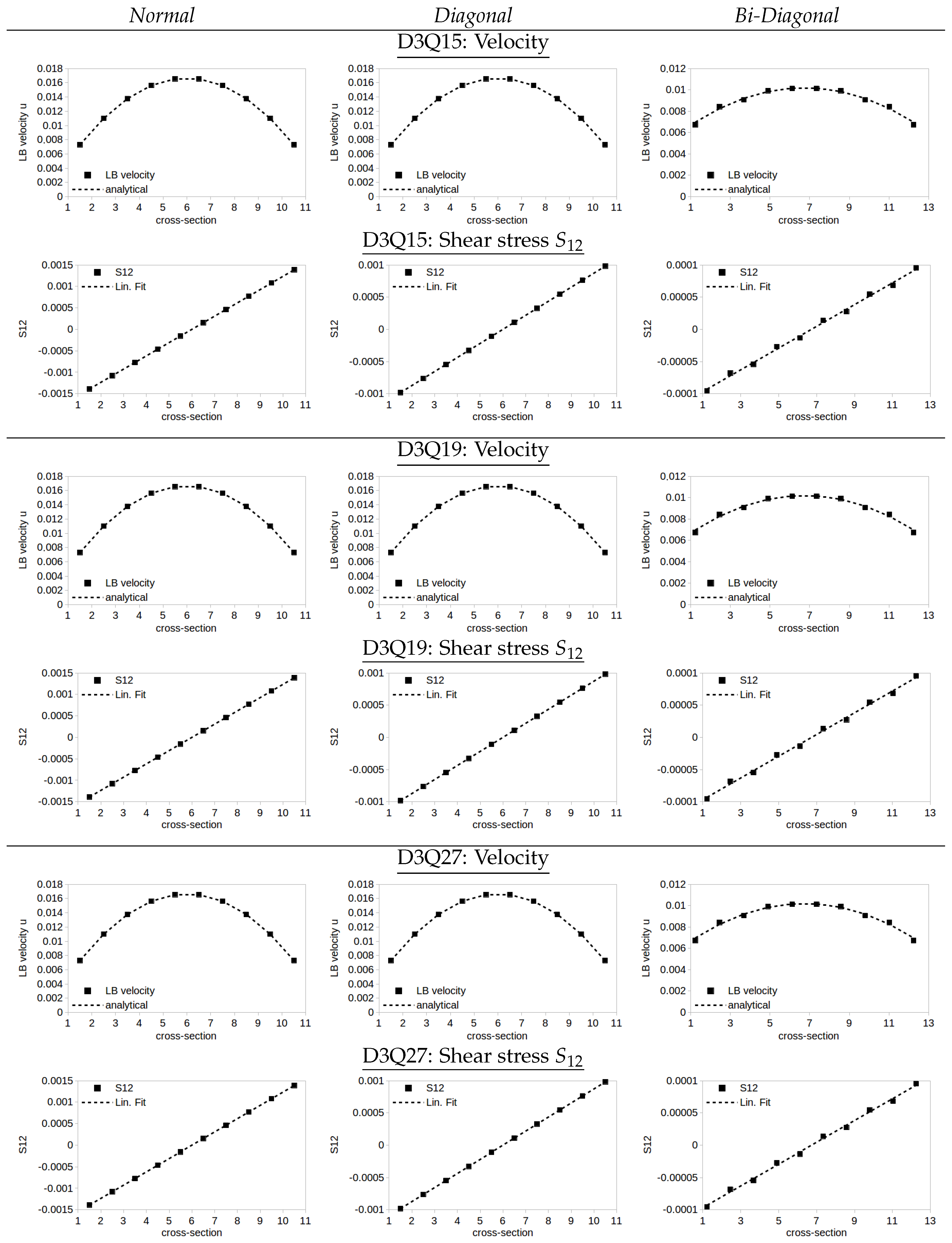
3.2. Validation: Optimization-Based LB Boundary Conditions

Given pressure/density, velocity and fluid stresses, we use the cell-local optimization-based boundary condition on LB side to specify the respective NS values. We validate this boundary treatment for the discretizations D3Q15, D3Q19, D3Q27 in three different scenarios of type “flow between two parallel infinite plates”, as illustrated in Figure 3. In all three setups, a cubic domain is considered, consisting of $10\times 10\times 10$ inner cells and one additional layer of boundary cells. We impose a parabolic velocity profile and linear pressure drop in the boundary cells of the cube: pressure, velocity values and stresses are specified as required by the optimization problem, cf. Equation (10). We consider a coordinate system aligned with the Cartesian LB grid. The setups are defined as follows:

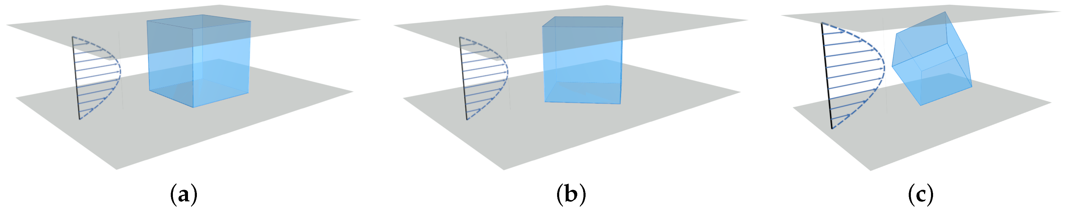
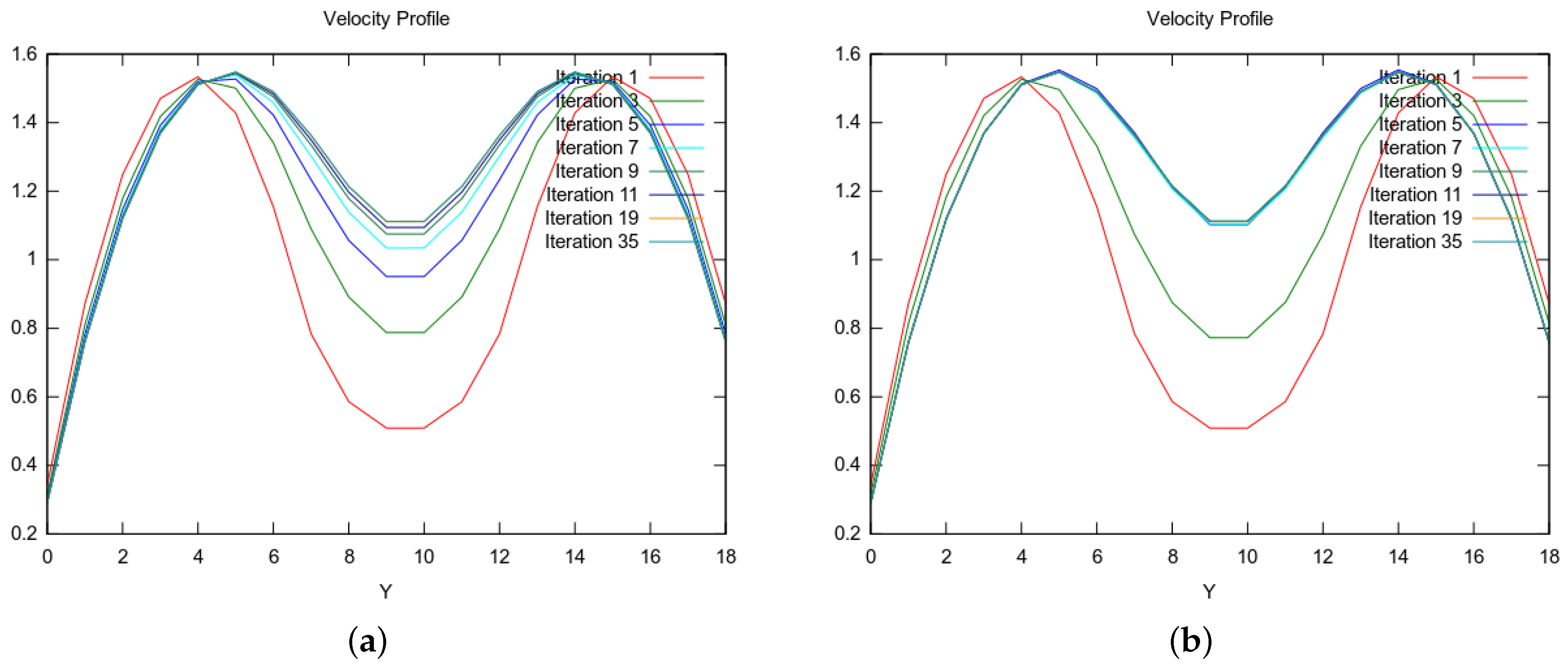
• Normal: the LB grid is aligned with the plates and the main flow direction, cf. Figure 3a. The main flow direction is thus given by ${(1,0,0)}^{\top }$.
• Diagonal: the LB grid is rotated ${45}^{\circ }$ away from the main flow axis and kept aligned with the plates, cf. Figure 3b. The main flow direction is hence parallel to ${(1,1,0)}^{\top }$.
• Bi-Diagonal: the LB grid is rotated such that only one corner is placed on each boundary plane, cf. Figure 3c. The main flow direction is aligned with ${(1,1,1)}^{\top }$, the normal of the plates is given by $\pm {\sqrt{6}}^{-1}{(1,-2,1)}^{\top }$.

The LB viscosity is set to ${\nu }^{LB}=1/6$. The avg. inlet velocity is given by $u^{LB}=0.05$ for Normal and Diagonal, and by $u^{LB}=0.05·\frac{\sqrt{6}}{4}$ for Bi-Diagonal to retain the same Reynolds number as in the other two setups. After reaching steady-state, the profiles of the velocity and the shear stress expression $S_{12}:={\displaystyle \sum _i}{f}_i^{neq}{\mathbf{c}}_{i_1}{\mathbf{c}}_{i_2}$ along the channel cross-section through the center point of the cubic simulation domain are evaluated.

The results for the different LB discretizations are shown in Figure 4. For all discretizations, both velocity and shear stress are captured correctly. The same holds for the linear pressure drop (not shown in Figure 4).

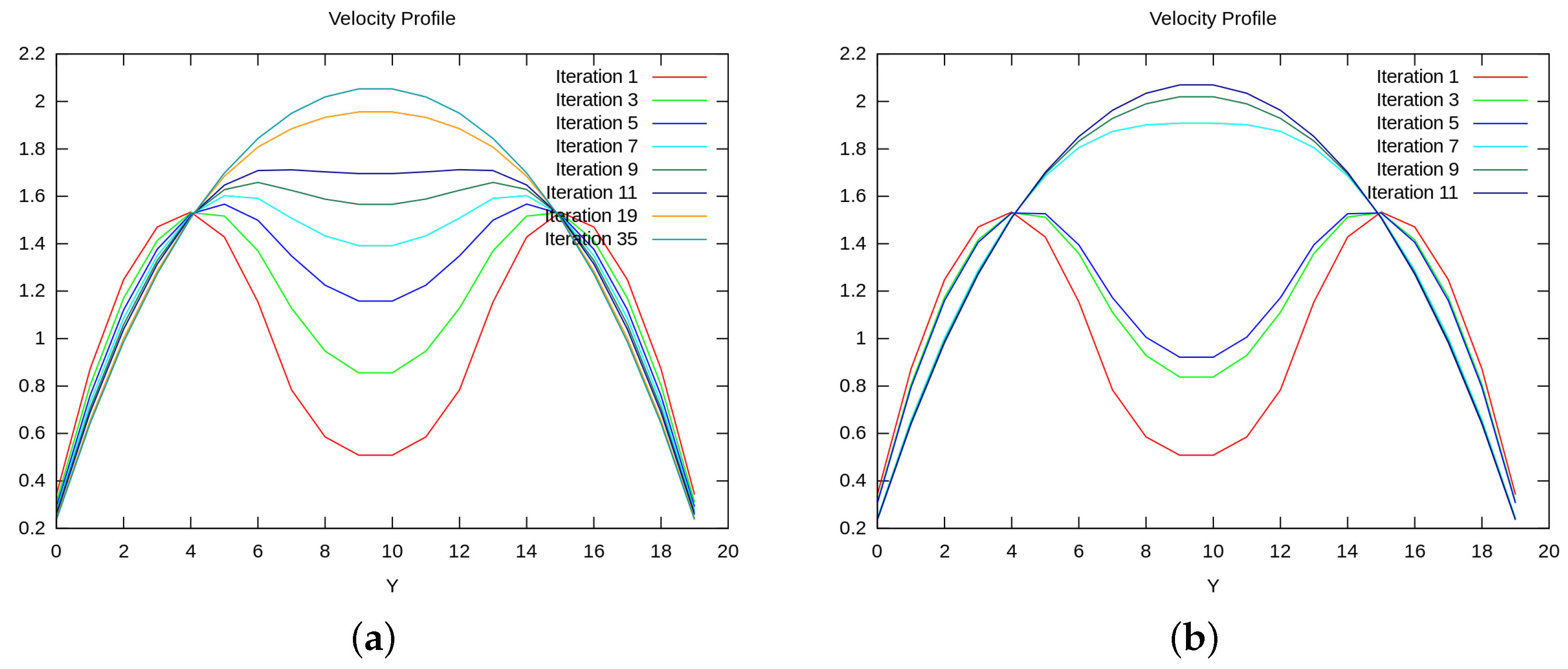
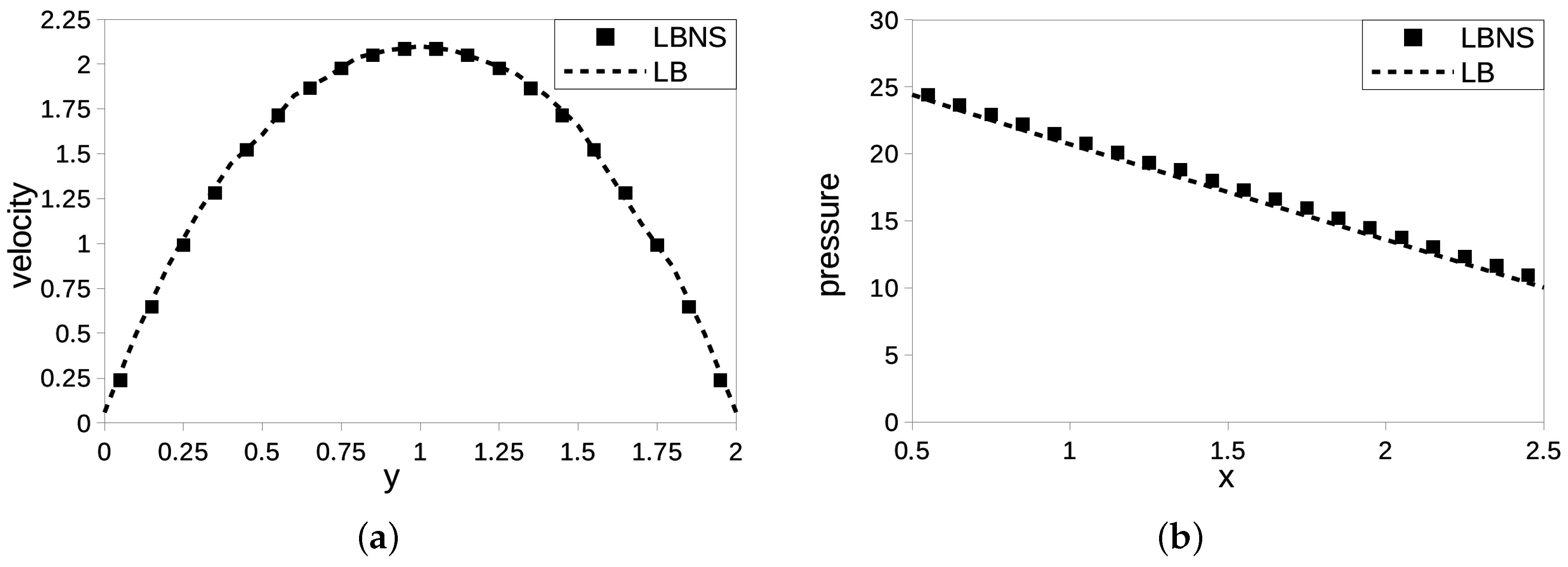
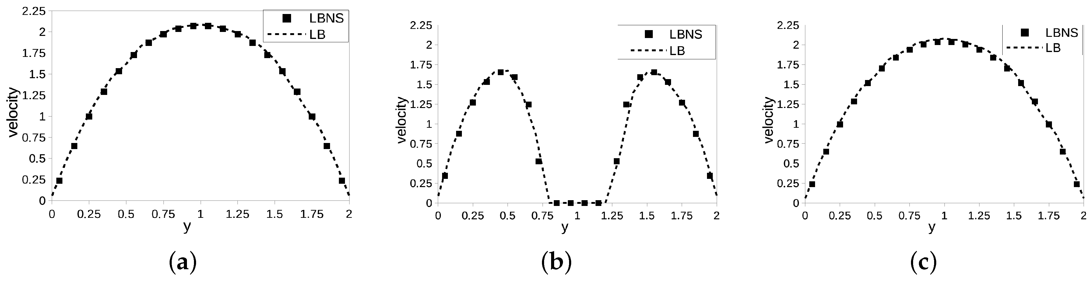
3.3. LBNS Validation: Plane Channel

For validation of the coupled scenario, we consider laminar flow in an empty channel. The channel has a box-like shape, stretching over $(l_x^{NS},l_y^{NS},l_z^{NS})=(4.0\times 2.0\times 2.0)$; the lower left front corner is located at $(0,0,0)$. In the NS simulation, the channel is discretized using $40\times 20\times 20$ cells, yielding a uniform mesh size $d{x}^{NS}=0.1$. The viscosity is set to $\nu =1.0$. On the left side, an inlet velocity profile

$$u^{NS}(x,y)=36\frac{u_c^{NS}}{l_y^2{l}_z^2}y(y-l_y)z(z-l_z)$$

(18)

is prescribed, with an average inlet velocity $u_c^{NS}=1.0$. Outlet conditions are imposed on the right side of the channel in form of a fixed pressure, $p^{NS}=0.0$. All walls are treated as no-slip boundaries. A cubic subdomain ranging from $(1.0,0.5,0.5)$ (lower left front corner) to $(2.0,1.5,1.5)$ (upper right back corner) is solved by the LB simulation, using a mesh size $d{x}^{LB}=0.25d{x}^{NS}=0.025$. The overlap region is chosen to have a thickness of two NS cells. The relaxation time in the BGK model is chosen as $\tau =1.0$.

With the parallel coupling exactly converging 50% slower than the sequential method, we restrict the considerations to the parallel coupling and the Anderson accelerated coupling. The Anderson acceleration starts “remembering and reusing” information only after one coupling cycle. Besides, the LB simulation is initialized at zero velocity and unit density, yielding a significantly different solution than the channel flow prediction of the NS solver in the first coupling cycle. For these reasons, we activate the Anderson acceleration after two coupling iterations. The different coupling methods (parallel/Anderson acceleration) converge towards the same solution, cf. Figure 5. The Anderson acceleration significantly speeds up the convergence. The velocity profiles are measured along a cross-section through the coupling region for the different coupling methods. After the first few iterations, the Anderson acceleration converges significantly faster than the sequential coupling. The overhead of the Anderson acceleration—compared to the parallel coupling scheme—amounts in the current (non-optimized) implementation to approx. 63% (computed from the average computational time over the first 10 coupling cycles). However, only 10–11 Anderson coupling iterations are required to reach an accurate description of the velocity profile, compared to 35 coupling iterations in the case of parallel coupling (17–18 coupling iterations in case of sequential coupling, respectively), cf. Figure 5. Since the Anderson acceleration allows for faster convergence in terms of coupling iterations and yields a better ratio of parallelizable to purely sequential tasks, we conclude that Anderson accelerated coupling is a promising candidate for massively parallel LBNS simulations.

We further computed the solution using LB everywhere in the channel at the same resolution $d{x}^{LB}$. Figure 6 shows good agreement between the pure LB and LBNS solution for both velocity profile and linear pressure drop.

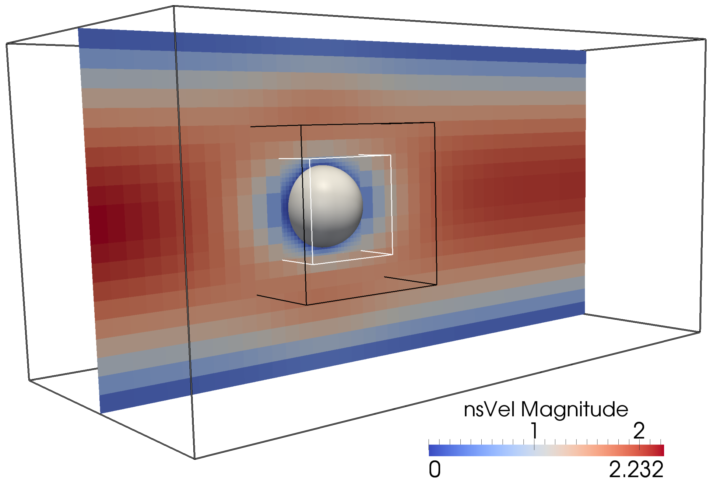
3.4. LBNS: Flow Past Spherical Obstacle

Next, we consider the same channel setup, cf. Section 3.3, and extend it by introducing a spherical obstacle in the middle of the LB domain. We use the half-way bounce back scheme to treat the spherical boundary as no-slip obstacle. The sphere is located at $(1.5,1.0,1.0)$ and has a radius $r=0.25$. The coupled setup is shown in Figure 7.

The three coupling schemes show similar convergence properties compared to the empty channel scenario, see Figure 8. We further compared the steady-state LBNS solution with the pure LB simulation. For this purpose, we consider the profiles before ($x=0.5$), at ($x=1.5$) and behind ($x=3.0$) the obstacle at respective cross-sections. As it can be seen from Figure 9, all profiles are in excellent agreement.

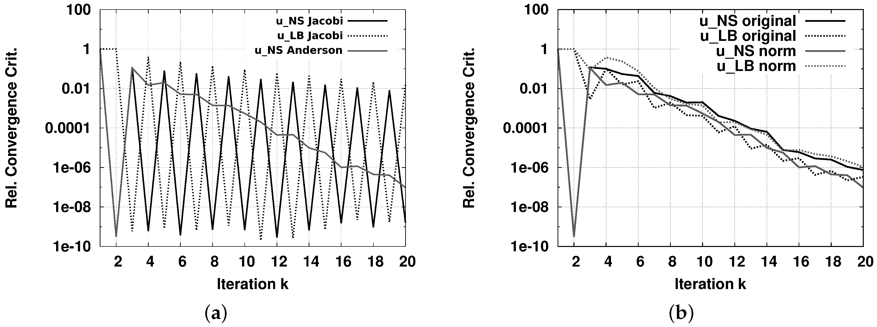
3.5. Anderson Acceleration: Parameter Study

In order to further evaluate the performance of the Anderson acceleration applied to our coupled simulation (cf. Section 2.3.4), we reconsider the plane channel scenario, cf. Section 3.3. We quantify the convergence rate using the relative convergence criterion

$$\frac{\parallel R^k{\parallel }_2}{\parallel {\tilde{x}}^k{\parallel }_2}\stackrel{!}{<}{ϵ}_{\mathrm{rel}}.$$

(19)

The criterion is evaluated for each coupling variable individually between two successive iterations. This yields a zick-zack-like convergence of both LB and NS solver for the parallel coupling, cf. Figure 10a. Both LB and NS solver converge at the same rate, but convergence is shifted by one iteration.

To avoid imbalances in the least-squares system of the Anderson acceleration, that is to put more weight on either LB or NS, we extend the formulation by normalizing the vectors of coupling variables ${\mathbf{u}}_{ovlp}^{NS}$, $p_{ovlp}^{NS}$, and ${\mathbf{u}}_{ovlp}^{LB}$. Slightly faster convergence is observed for the normalized variants compared to the original scheme, see Figure 10b. The first zick-zack of the parallel coupling is also visible in this case, due to the initialization of the coupled setup: zero velocity is initially imposed in the LB region, and at least one coupling iteration is required to transport flow information from NS into the LB region. Since this still implies very low velocities in the LBNS overlap, the solution and thus the convergence rate are hardly affected. The mean speed of convergence of the normalized Anderson accelerated coupling is significantly faster than for the parallel coupling, see Figure 10a.

Table 1. Influence of normalization and the choice of primary and secondary variables for the Anderson accelerated coupling. Runs with only one primary coupling variable do not converge. The bold numbers in columns 4,5 correspond to the absolute number of coupling iterations (maximum of the given iteration numbers for each coupling variable) to reach convergence. We use dim(${\mathbf{u}}_{ovlp}^{NS})=302580$ and dim(${\mathbf{u}}_{ovlp}^{LB})=5760$.

Primary	Secondary	Norm.	Iterations till ${10}^{-5}$	Iterations till ${10}^{-7}$
			(${\mathbf{u}}^{NS}$/${\mathbf{u}}_{ovlp}^{LB}$/$p_{ovlp}^{NS}$)	(${\mathbf{u}}_{ovlp}^{NS}$/${\mathbf{u}}_{ovlp}^{LB}$/$p_{ovlp}^{NS}$)
${\mathbf{u}}_{ovlp}^{NS}$, ${\mathbf{u}}_{ovlp}^{LB}$	$p_{ovlp}^{NS}$	no	15 / 13 / 15	23 / 21 / 23
${\mathbf{u}}_{ovlp}^{NS}$, ${\mathbf{u}}_{ovlp}^{LB}$	$p_{ovlp}^{NS}$	yes	14 / 15 / 14	20 / 23 / 20
${\mathbf{u}}_{ovlp}^{NS}$, ${\mathbf{u}}_{ovlp}^{LB}$, $p_{ovlp}^{NS}$	-	yes	15 / 15 / 15	22 / 23 / 22
$p_{ovlp}^{NS}$, ${\mathbf{u}}_{ovlp}^{LB}$	${\mathbf{u}}_{ovlp}^{NS}$	yes	14 / 17 / 14	22 / 24 / 22

lists the number of iterations that different Anderson acceleration approaches need to converge below a threshold of ${10}^{-5}$ and ${10}^{-7}$. The maximum number of iterations in ${\mathbf{u}}_{ovlp}^{NS}$, ${\mathbf{u}}_{ovlp}^{NS}$ or $p_{ovlp}^{NS}$ (shown as bold number in Table 1) dictates the overall number of iterations that are required for convergence. Similarly, in

Table 2. Influence of the ratio, and of the normalization on the convergence behavior of the Anderson accelerated coupling. All runs use ${\mathbf{u}}_{ovlp}^{NS}$ and ${\mathbf{u}}_{ovlp}^{LB}$ as primary variables, and $p_{ovlp}^{NS}$ as a secondary variable. The mesh is coarsened by a factor of two compared to the results in Table 1. The bold numbers in columns 5,6 correspond to the absolute number of coupling iterations (maximum of the given iteration numbers for each coupling variable) to reach convergence.

Ratio	dim(${\mathbf{u}}_{\mathit{o}\mathit{v}\mathit{l}\mathit{p}}^{\mathit{N}\mathit{S}}$)	dim(${\mathbf{u}}_{\mathit{o}\mathit{v}\mathit{l}\mathit{p}}^{\mathit{L}\mathit{B}}$)	Norm.	Iterations till ${10}^{-5}$	Iterations till ${10}^{-7}$
				(${\mathbf{u}}_{ovlp}^{NS}$/${\mathbf{u}}_{ovlp}^{LB}$/$p_{ovlp}^{NS}$)	(${\mathbf{u}}_{ovlp}^{NS}$/${\mathbf{u}}_{ovlp}^{LB}$/$p_{ovlp}^{NS}$)
1	10080	460	no	9 / 9 / 9	12 / 13 / 12
1	10080	460	yes	8 / 10 / 8	12 / 13 / 16
2	34980	460	no	10 / 7 / 10	13 / 11 / 13
2	34980	460	yes	8 / 10 / 8	12 / 14 / 13
4	129780	460	no	11 / 7 / 10	14 / 13 / 17
4	129780	460	yes	8 / 11 / 8	13 / 15 / 17
8	499380	460	no	11 / 7 / 11	16 / 14 / 16
8	499380	460	yes	8 / 11 / 8	14 / 15 / 14

, we study the effect of different ratios of Lattice Boltzmann to Navier–Stokes cells on the convergence rate. Several aspects can be observed in both tables and are detailed in the following.

Normalizing the vectors of coupling variables has an influence on the convergence speed, and can shift the bias from the Navier–Stokes to the Lattice Boltzmann variables and vice versa, compare also Figure 10b. This influence, however, is very limited in this example which is mainly due to the fact that all coupling variables already live on the same characteristic physical scale. Furthermore, Table 1 shows that the normalization is not necessarily the optimal balance. Due to its very limited influence, we omit further detailed studies here.

If only coupling variables of one solver are considered, the coupling information is incomplete, and the overall scheme does not converge in this case.

Consider Table 1. Introducing $p_{ovlp}^{NS}$ as a third primary coupling variable does not imply faster convergence. Apparently, this does not result in new information compared to ${\mathbf{u}}_{ovlp}^{NS}$. We can even observe a slight decrease in the overall convergence due to an imbalance in LB and NS information within the least-squares system.

Consider Table 1. If $p_{ovlp}^{NS}$ is used as a primary variable instead of ${\mathbf{u}}_{ovlp}^{NS}$, we observe a slightly slower convergence. This substitution, however, reduces the size of the least-squares system by a factor of ∼3 (the size of the vector ${\mathbf{u}}_{ovlp}^{LB}\in {\mathbb{R}}^{5760}$ is much smaller than the size of ${\mathbf{u}}_{ovlp}^{NS}\in {\mathbb{R}}^{302580}$ in this example).

Consider Table 2. The ratio of of Lattice Boltzmann and Navier–Stokes cells in the overlap region has no significant influence on the convergence behavior.

We conclude from this parameter study that the usage of the two velocity vectors ${\mathbf{u}}_{ovlp}^{NS}$ and ${\mathbf{u}}_{ovlp}^{LB}$ as primary variables is recommended. A substitution of ${\mathbf{u}}_{ovlp}^{NS}$ by $p_{ovlp}^{NS}$ can be useful for scenarios, where the size of the least-squares system matters, i.e., scenarios with a big overlap region compared to the overall domain. The normalization of coupling variables as well as the ratio between the number of Lattice Boltzmann and Navier–Stokes cells have little influence on the convergence behavior.

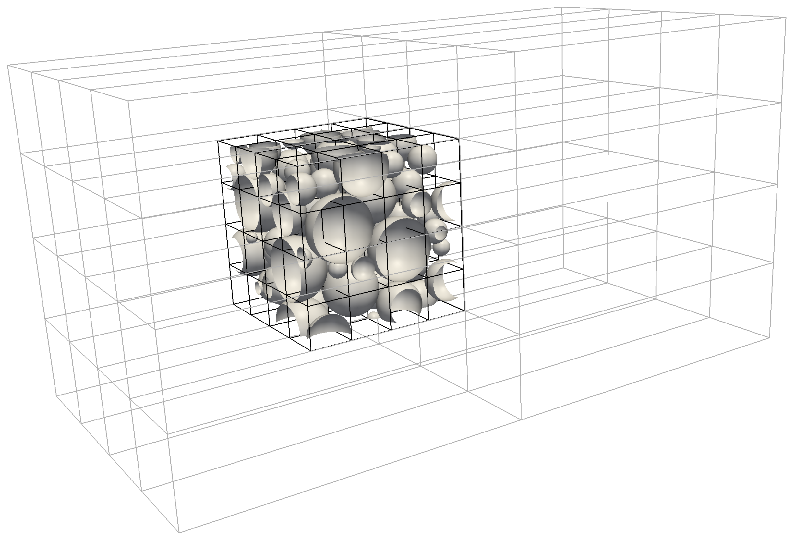
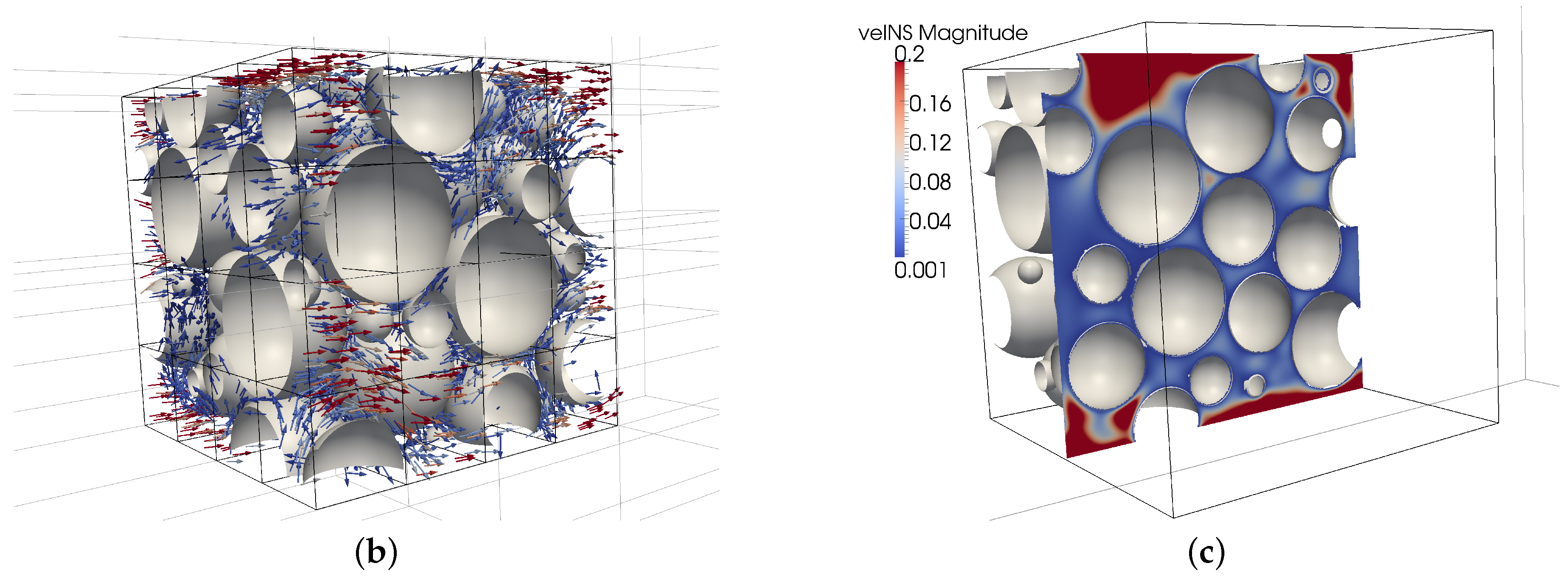
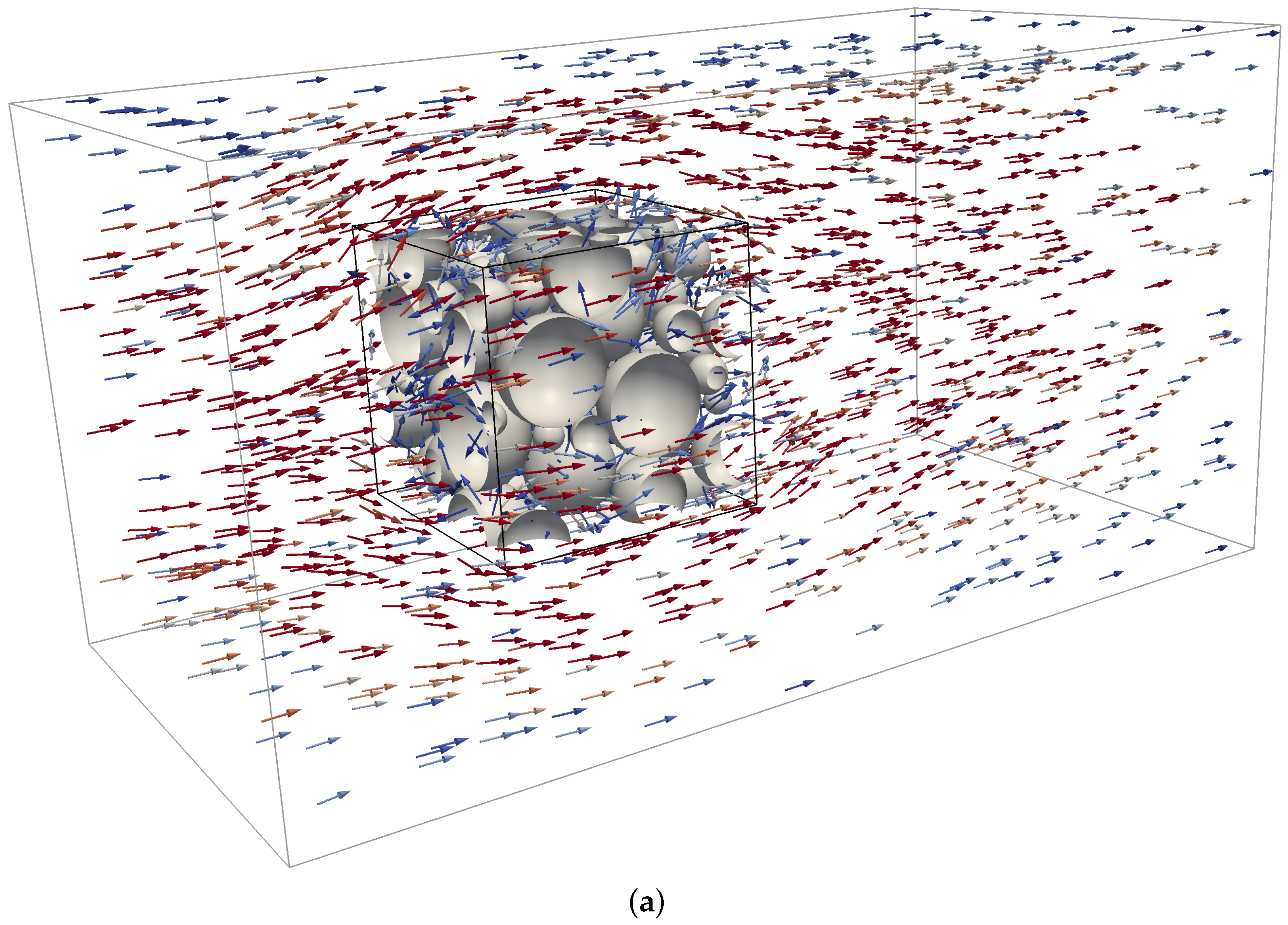
3.6. LBNS Showcase: Flow in Porous Structures

Finally, we apply the LBNS methodology to flow through a porous structure [5,37,38], pointing out the applicability of our method to parallel (component-based) simulations with complex geometries. The setup is shown in Figure 11 and consists of a channel domain Ω of size $32.0\times 16.0\times 16.0$ with a set of 100 random-sized rigid spheres packed inside a volume ${\mathsf{\Omega }}^{LB}$ of $8.0\times 8.0\times 8.0$. This volume, i.e., its lower left front corner, is located at $8.0\times 4.0\times 4.0$. Due to the complex geometry of the porous medium-like sphere packing, we apply the highly localized LB method in this region ${\mathsf{\Omega }}^{LB}$. The rest of the channel ${\mathsf{\Omega }}^{NS}=\mathsf{\Omega }\setminus {\mathsf{\Omega }}^{LB}$ is solved by NS. We discretize ${\mathsf{\Omega }}^{NS}$ with Cartesian grid cells of equidistant size $d{x}^{NS}=0.1$ and ${\mathsf{\Omega }}^{LB}$ with cells of size $d{x}^{LB}=d{x}^{NS}/4=0.025$ respectively, resulting in $320\times 160\times 160$ NS and $321\times 321\times 321$ LB nodes. The fluid parameters are chosen as $\nu =1.0$ and $\tau =1.0$, the avg. inlet velocity is set to $u_c^{NS}=1.0$. Ten iterations of the parallel coupling scheme are carried out using 32 NS processes and 64 LB processes. A visualization of the flow field around and in the porous structure after the tenth coupling iteration is shown in Figure 12.

4. Conclusions

We presented a novel spatial coupling method for fully three-dimensional, steady-state simulations. The method combines Lattice Boltzmann and incompressible Navier–Stokes solvers and allows to locally exploit the features of each simulation approach. We validated the LB boundary conditions used in the LBNS overlap region, studied the Anderson acceleration method for LBNS coupling and compared it to purely sequential and simple Schwarz-based parallel coupling schemes. All coupling schemes converged in the presented test cases, i.e., plane channel flow and flow past a spherical obstacle, towards the expected solution. The Anderson acceleration method showed very good performance in terms of convergence rates which clearly outperformed the sequential and simple parallel coupling (11 vs. 18/35 coupling cycles, cf. Section 3.3). We currently work towards incorporating the iterative LBNS coupling into transient LBNS simulations to investigate whether this approach reduces any compressibility perturbations in the flow field. Besides, more detailed studies are required in future to evaluate the influence of normalization of the different coupling vectors (cf. Section 3.5). Although the influence was limited in the presented study, it may become more significant in case of more complex scenarios, or in case of bigger gradients in the coupling region.

References

1. Ferziger, J.; Perić, M. Computational Methods for Fluid Dynamics, 2nd ed.; Springer: Berlin/Heidelberg, Germany, 1999. [Google Scholar]
2. Fletcher, C. Computational Techniques for Fluid Dynamics, Volume 2: Specific Techniques for Different Flow Categories, 2nd ed.; Springer: Berlin, Germany, 1997. [Google Scholar]
3. Succi, S. The Lattice Boltzmann Equation for Fluid Dynamics and Beyond; Oxford University Press: Oxford, UK, 2001. [Google Scholar]
4. Wolf-Gladrow, D. Lattice-Gas Cellular Automata and Lattice Boltzmann Models—An Introduction; Springer: Berlin, Germany, 2000. [Google Scholar]
5. Geller, S.; Krafczyk, M.; Tölke, J.; Turek, S.; Hron, J. Benchmark computations based on lattice-Boltzmann, finite element and finite volume methods for laminar flows. Comput. Fluids 2006, 35, 888–897. [Google Scholar] [CrossRef]
6. Mehl, M.; Neckel, T.; Neumann, P. Navier–Stokes and Lattice-Boltzmann on octree-like grids in the Peano framework. Int. J. Numer. Methods Fluids 2010, 65, 67–86. [Google Scholar] [CrossRef]
7. Junk, M.; Klar, A.; Luo, L.S. Asymptotic analysis of the lattice Boltzmann equation. J. Comput. Phys. 2005, 210, 676–704. [Google Scholar] [CrossRef]
8. Chen, L.; He, Y.L.; Kang, Q.; Tao, W.Q. Coupled numerical approach combining finite volume and lattice Boltzmann methods for multi-scale multi-physicochemical processes. J. Comput. Phys. 2013, 255, 83–105. [Google Scholar] [CrossRef]
9. Latt, J.; Chopard, B.; Albuquerque, P. Spatial Coupling of a Lattice Boltzmann fluid model with a Finite Difference Navier–Stokes solver. 2005; arXiv:physics/0511243. Available online: http://xxx.lanl.gov/abs/physics/0511243 (accessed on 11 October 2016). [Google Scholar]
10. Neumann, P. Hybrid Multiscale Simulation Approaches for Micro- and Nanoflows. Ph.D. Thesis, Technische Universität München, Institut für Informatik, Munich, Germany, 2013. [Google Scholar]
11. Neumann, P.; Bungartz, H.-J.; Mehl, M.; Neckel, T.; Weinzierl, T. A Coupled Approach for Fluid Dynamic Problems Using the PDE Framework Peano. Commun. Comput. Phys. 2012, 12, 65–84. [Google Scholar] [CrossRef]
12. Yeshala, N. A Coupled Lattice-Boltzmann–Navier–Stokes Methodology for Drag Reduction. Ph.D. Thesis, Georgia Institute of Technology, Atlanta, GA, USA, 2010. [Google Scholar]
13. Albuquerque, P.; Alemani, D.; Chopard, B.; Leone, P. Coupling a Lattice Boltzmann and a Finite Difference Scheme. In Computational Science–ICCS 2004; Springer: Berlin/Heidelberg, Germany, 2004; pp. 540–547. [Google Scholar]
14. Albuquerque, P.; Alemani, D.; Chopard, B.; Leone, P. A Hybrid Lattice Boltzmann Finite Difference Scheme for the Diffusion Equation. Int. J. Mult. Comp. Eng. 2006, 4, 209–219. [Google Scholar]
15. Neumann, P. On transient hybrid Lattice Boltzmann–Navier–Stokes flow simulations. J. Comput. Sci. 2016, in press. [Google Scholar] [CrossRef]
16. Degroote, J.; Bathe, K.; Vierendeels, J. Performance of a new partitioned procedure versus a monolithic procedure in fluid-structure interaction. Comput. Struct. 2009, 87, 793–801. [Google Scholar] [CrossRef]
17. Lott, P.; Walker, H.; Woodward, C.; Yang, U. An accelerated Picard method for nonlinear systems related to variably saturated flow. Adv. Water Resour. 2012, 38, 92–101. [Google Scholar] [CrossRef]
18. Ni, P. Anderson Acceleration of Fixed-Point Iteration with Applications to Electronic Structure Computations. Ph.D. Thesis, Worcester Polytechnic Institute, Worcester, MA, USA, 2009. [Google Scholar]
19. Anderson, D.G. Iterative procedures for nonlinear integral equations. J. ACM 1965, 12, 547–560. [Google Scholar] [CrossRef]
20. Fang, H.; Saad, Y. Two classes of multisecant methods for nonlinear acceleration. Numer. Linear Algebra Appl. 2009, 16, 197–221. [Google Scholar] [CrossRef]
21. Walker, H.; Ni, P. Anderson acceleration for fixed-point iterations. SIAM J. Numer. Anal. 2011, 49, 1715–1735. [Google Scholar] [CrossRef]
22. Shan, X. Lattice Boltzmann in micro- and nano-flow simulations. IMA J. Appl. Math. 2011, 76, 650–660. [Google Scholar] [CrossRef]
23. Meng, J.; Zhang, Y.; Shan, X. Multiscale lattice Boltzmann approach to modeling gas flows. Phys. Rev. E 2011, 83, 046701. [Google Scholar] [CrossRef] [PubMed]
24. Dünweg, B.; Schiller, U.; Ladd, A. Statistical Mechanics of the Fluctuating Lattice Boltzmann Equation. Phys. Rev. E 2007, 76, 036704. [Google Scholar] [CrossRef] [PubMed]
25. Griebel, M.; Dornseifer, T.; Neunhoeffer, T. Numerical Simulation in Fluid Dynamics. A Practical Introduction; SIAM: Philadelphia, PA, USA, 1997. [Google Scholar]
26. Bhatnagar, P.; Gross, E.; Krook, M. A Model for Collision Processes in Gases. I. Small Amplitude Processes in Charged and Neutral One-Component Systems. Phys. Rev. 1954, 94, 511–525. [Google Scholar] [CrossRef]
27. Chapman, S.; Cowling, T. The Mathematical Theory of Nonuniform Gases; Cambridge University Press: London, UK, 1970. [Google Scholar]
28. Zou, Q.; He, X. On pressure and velocity boundary conditions for the lattice Boltzmann BGK model. Phys. Fluids 1997, 9, 1591–1598. [Google Scholar] [CrossRef]
29. Latt, J.; Chopard, B.; Malaspinas, O.; Deville, M.; Michler, A. Straight velocity boundaries in the lattice Boltzmann method. Phys. Rev. E 2008, 77. [Google Scholar] [CrossRef] [PubMed]
30. Chikatamarla, S.; Ansumali, S.; Karlin, I. Grad’s approximation for missing data in lattice Boltzmann simulations. Europhys. Lett. 2006, 74, 215–221. [Google Scholar] [CrossRef]
31. Schwarz, H. Ueber einen Grenzübergang durch alternierendes Verfahren. Vierteljahrsschrift der Naturforschenden Gesellschaft Zürich 1870, 15, 272–286. (In German) [Google Scholar]
32. Uekermann, B.; Bungartz, H.-J.; Gatzhammer, B.; Mehl, M. A parallel, black-box coupling algorithm for fluid-structure interaction. In Proceedings of the 5th International Conference on Computational Methods for Coupled Problems in Science and Engineering, Ibiza, Spain, 17–19 June 2013; pp. 1–12.
33. Atanasov, A. Software Idioms for Component-Based and Topology-Aware Simulation Assembly and Data Exchange in High Performance Computing and Visualisation Environments. Ph.D. Thesis, Technische Universität München, Institut für Informatik, Munich, Germany, 2014. [Google Scholar]
34. Atanasov, A.; Bungartz, H.-J.; Unterweger, K.; Weinzierl, T.; Wittmann, R. A Case Study on Multi-Component Multi-Cluster Interaction with an AMR Solver. In Proceedings of the Third International Workshop on Domain-Specific Languages and High-Level Frameworks for High Performance Computing (WOLFHPC 2013), Denver, CO, USA, 18 November 2013.
35. Balay, S.; Adams, M.F.; Brown, J.; Brune, P.; Buschelman, K.; Eijkhout, V.; Gropp, W.D.; Kaushik, D.; Knepley, M.G.; McInnes, L.C.; et al. PETSc Web Page. Available online: http://www.mcs.anl.gov/petsc (accessed on 17 November 2014).
36. Bungartz, H.-J.; Lindner, F.; Gatzhammer, B.; Mehl, M.; Scheufele, K.; Shukaev, A.; Uekermann, B. preCICE—A Fully Parallel Library for Multi-Physics Surface Coupling. Comput. Fluids 2016, in press. [Google Scholar] [CrossRef]
37. Khirevich, S.; Ginzburg, I.; Tallarek, U. Coarse- and fine-grid numerical behavior of MRT/TRT lattice-Boltzmann schemes in regular and random sphere packings. J. Comput. Phys. 2014, 281, 708–742. [Google Scholar] [CrossRef]
38. Grucelski, A.; Pozorski, J. Lattice Boltzmann simulations of flow past a circular cylinder and in simple porous media. Comput. Fluids 2013, 71, 406–416. [Google Scholar] [CrossRef]
Figure 1. Decomposition of the computational domain into subdomains Ω N S and Ω L B for the NS and LB solver, and an overlap region Ω O v l p .
Computation 04 00038 g001
Figure 2. Grids and interpolation rules. (a) Interpolation of LB values. The outer red-colored nodes correspond to the LB boundary layer. The surrounding NS values in- and outside the (gray-colored) overlap region are used to interpolate density, velocity and shear stresses on these LB nodes; (b) Interpolation of NS values. The LB nodes marked as red crosses are used to interpolate the velocity values at the marked green locations of the staggered NS grid.
Computation 04 00038 g002
Figure 3. Test setups for the optimization-based boundary treatment in the LB solver. The blue region corresponds to the Cartesian grid-based computational domain used by the LB solver, the direction of the parabolic flow profile is sketched on the left side of the gray plates. (a) Setup Normal; (b) Setup Diagonal; (c) Setup Bi-Diagonal.
Computation 04 00038 g003
Figure 4. Velocity and stress profiles in setups Normal, Diagonal, Bi-Diagonal for discretizations D3Q15, D3Q19, D3Q27. The best approximation “Lin. Fit” matches the analytic solution within a tolerance of ≤1%. The small oscillations in the setup Bi-Diagonal stem from the evaluation and data extraction of flow quantities from the Cartesian grid data structure, abstaining from interpolation despite the consideration of a rotated system.
Computation 04 00038 g004
Figure 5. Convergence of the velocity profile at cross-section through empty channel at ( 1 . 5 , y · d x N S , 1 . 0 ) , y [ 0 , 20 ] , towards steady state. (a) Simple parallel coupling; (b) Anderson accelerated parallel coupling.
Computation 04 00038 g005
Figure 6. Pressure and velocity profile in channel flow for LB and LBNS. (a) Velocity profile at cross-section ( 1 . 5 , y , 1 . 0 ) , y [ 0 . 0 , 2 . 0 ] ; (b) Pressure profile along centerline of the channel ( x , 1 . 0 , 1 . 0 ) , x [ 0 . 5 , 2 . 5 ] .
Computation 04 00038 g006
Figure 7. Steady-state velocity field for the LBNS scenario for flow past a spherical obstacle. The inner black-framed box shows the LB simulation domain, the region between inner black- and white-framed box corresponds to the overlap region.
Computation 04 00038 g007
Figure 8. Convergence of the velocity profile for channel flow past a spherical obstacle at cross-section at x = 2 . 0 , y [ 0 . 0 , 2 . 0 ] towards steady state. (a) Simple parallel coupling; (b) Anderson accelerated coupling.
Computation 04 00038 g008
Figure 9. Velocity profile at different cross-sections for channel flow past a spherical obstacle obtained from LB and LBNS simulations. (a) ( 0 . 5 , y , 1 . 0 ) ; (b) ( 1 . 5 , y , 1 . 0 ) ; (c) ( 3 . 0 , y , 1 . 0 ) , y [ 0 , 2 . 0 ] .
Computation 04 00038 g009
Figure 10. (a) Relative convergence criterion of the simple parallel (Jacobi-type) coupling scheme compared to the Anderson acceleration scheme (normalized, primary: u o v l p N S , u o v l p L B , secondary: p o v l p N S ); (b) Relative convergence criterion of the Anderson acceleration scheme. Normalized coupling variables are compared to the original values (primary: u o v l p N S , u o v l p L B , secondary: p o v l p N S ).
Computation 04 00038 g010
Figure 11. Channel flow with 100 random-sized rigid spherical obstacles forming a porous structure. The gray and black lines indicate the domain decomposition of NS and LB solver.
Computation 04 00038 g011
Figure 12. Visualization of the flow field of the channel flow with porous structure. (a) Flow field of the whole computational domain; (b) Flow field inside the porous structure; (c) Cut through the velocity field at y = 8 . 0 in porous structure. v e l N S M a g n i t u d e corresponds to the magnitude of the velocity in NS units.
Computation 04 00038 g012aComputation 04 00038 g012b