
Simplification of Reaction Networks, Confluence and Elementary Modes


Abstract
:1. Introduction
Outline
2. Preliminaries
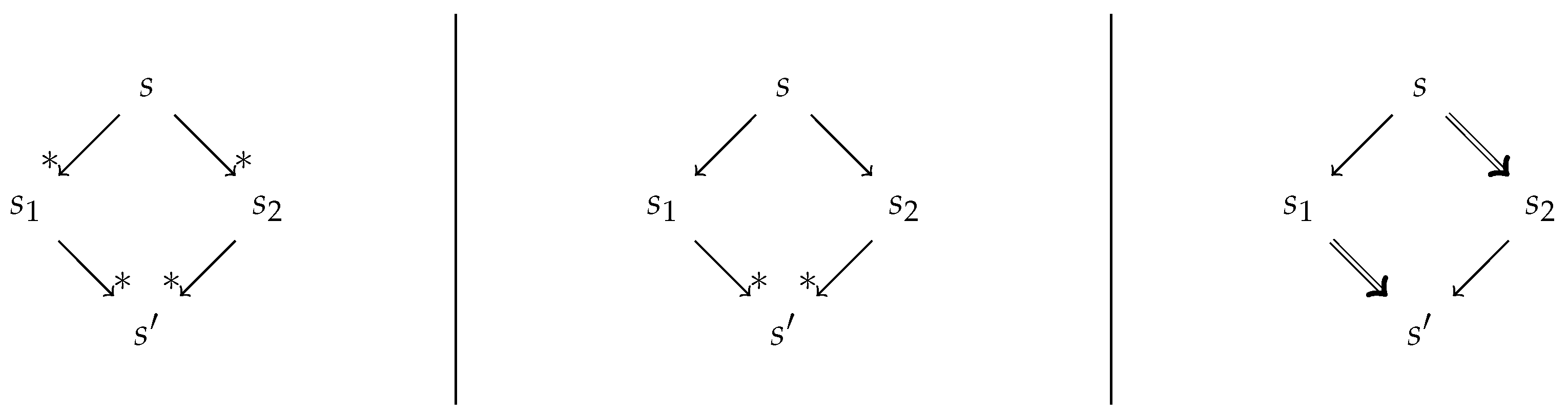
2.1. Confluence Notions
2.2. Multisets
2.3. Commutative Semigroups
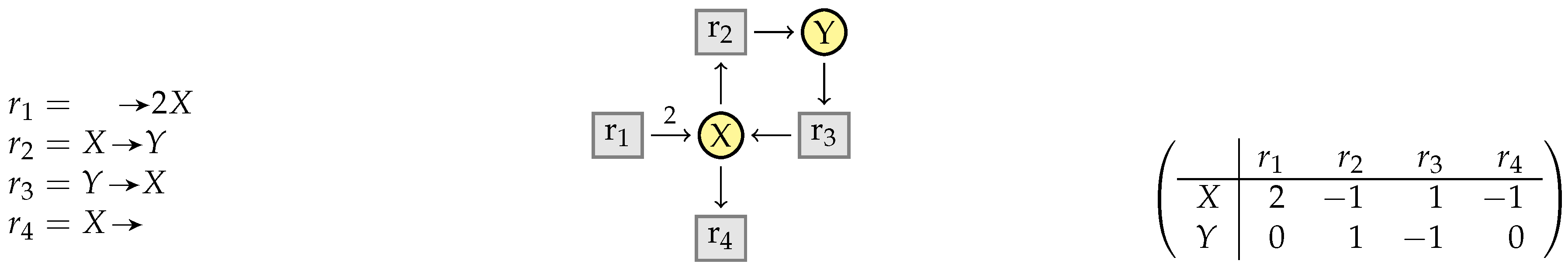
3. Reaction Networks without Kinetics
3.1. Stoichiometry Matrices
3.2. Elementary Modes
- v is on an extreme ray: there exists no such that , and
- v is factorised: there exists no such that for some natural number .
3.3. Elementary Flux Modes
4. Simplifying Reaction Networks without Kinetics
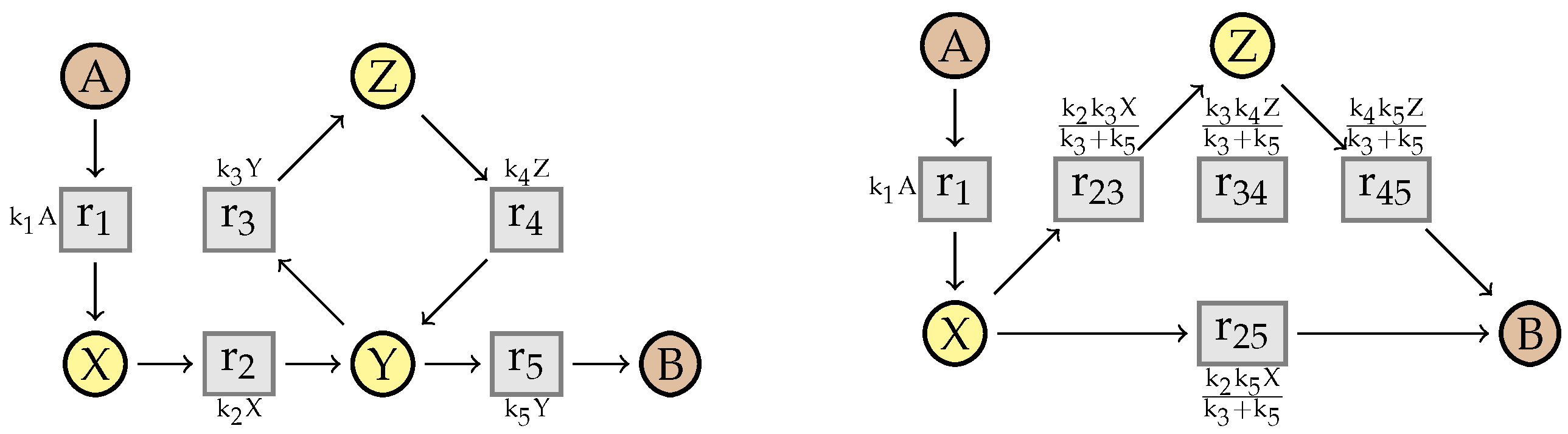
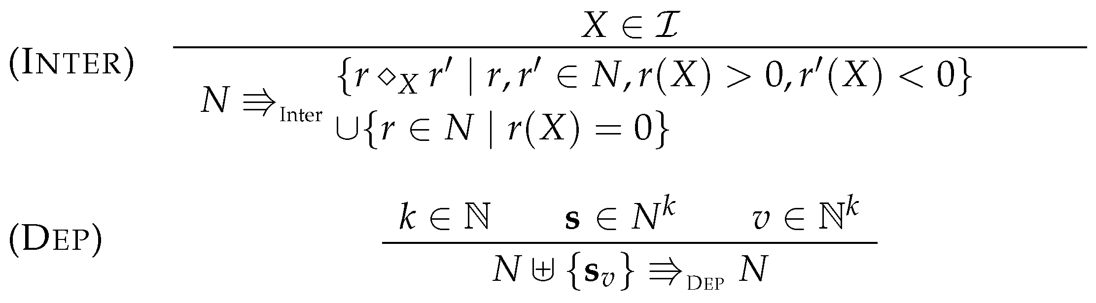
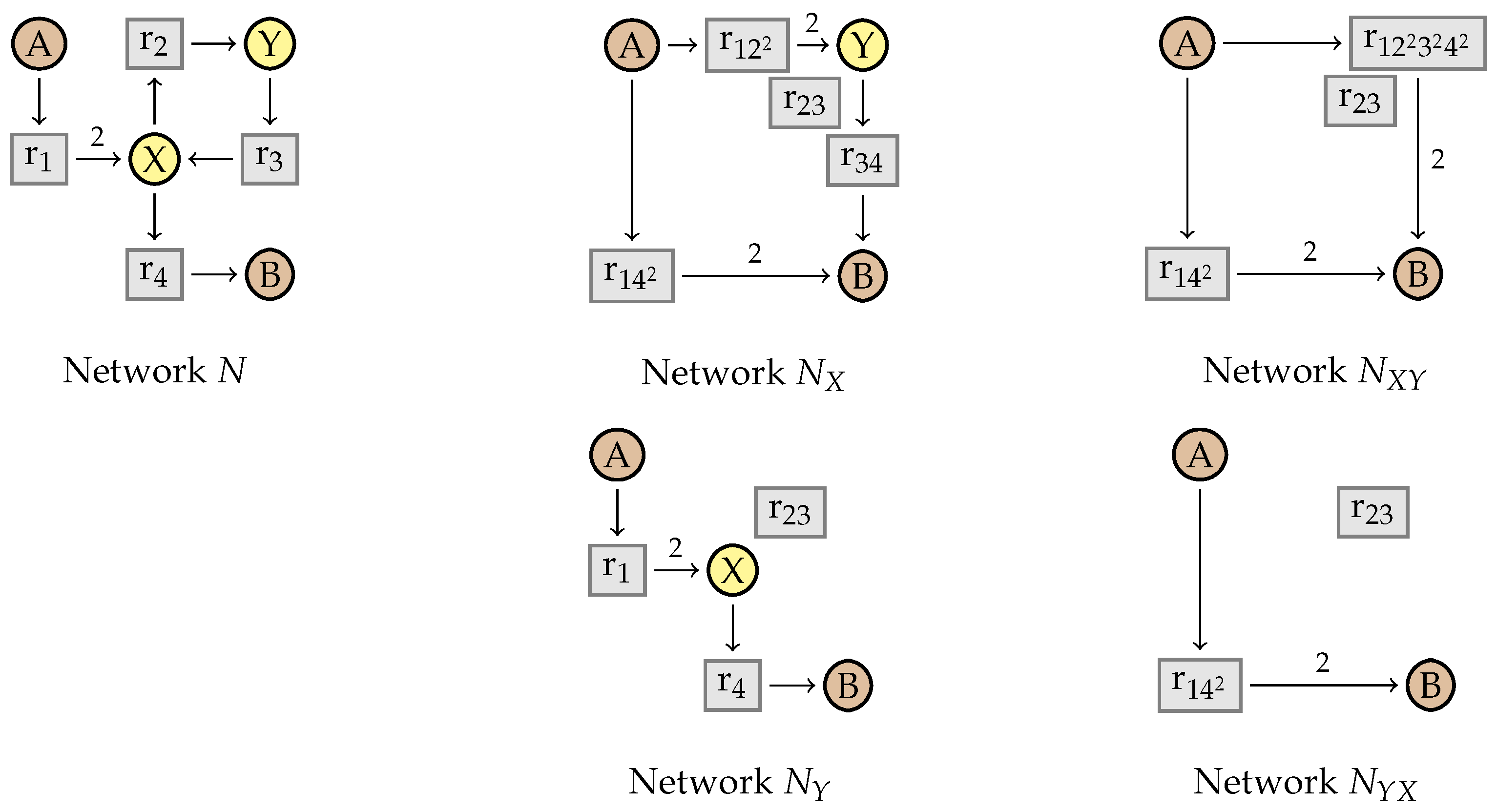
4.1. Intermediate Elimination
4.2. Eliminating Dependent Reactions
5. Simplifying Flux Networks
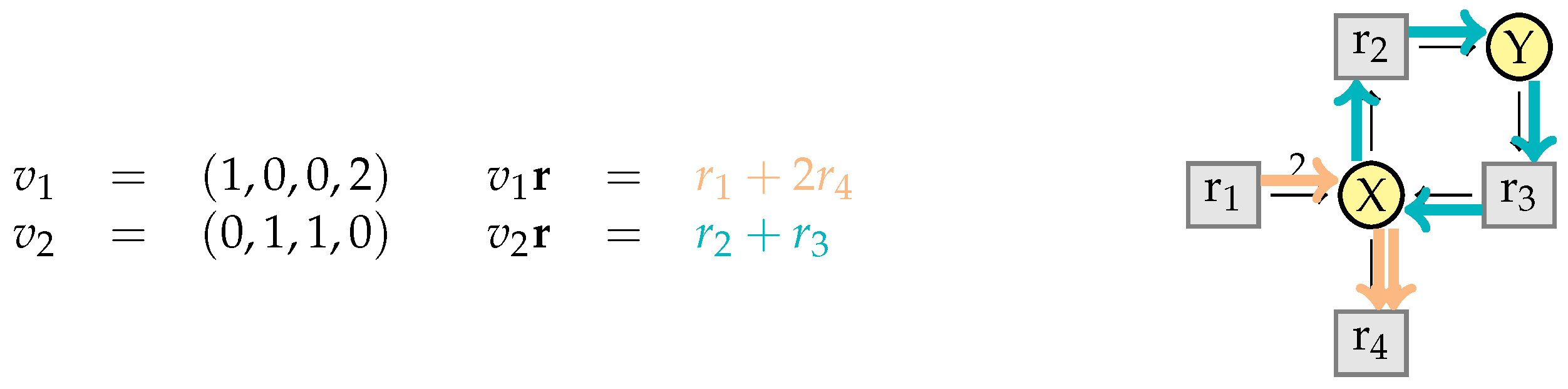
5.1. Vector Representations of Reaction Networks
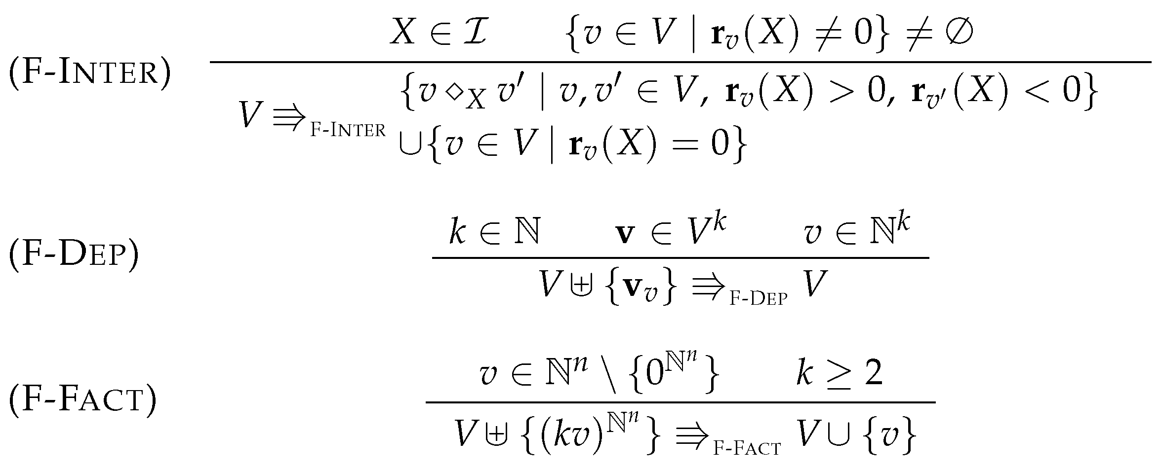
5.2. Simplification Rules
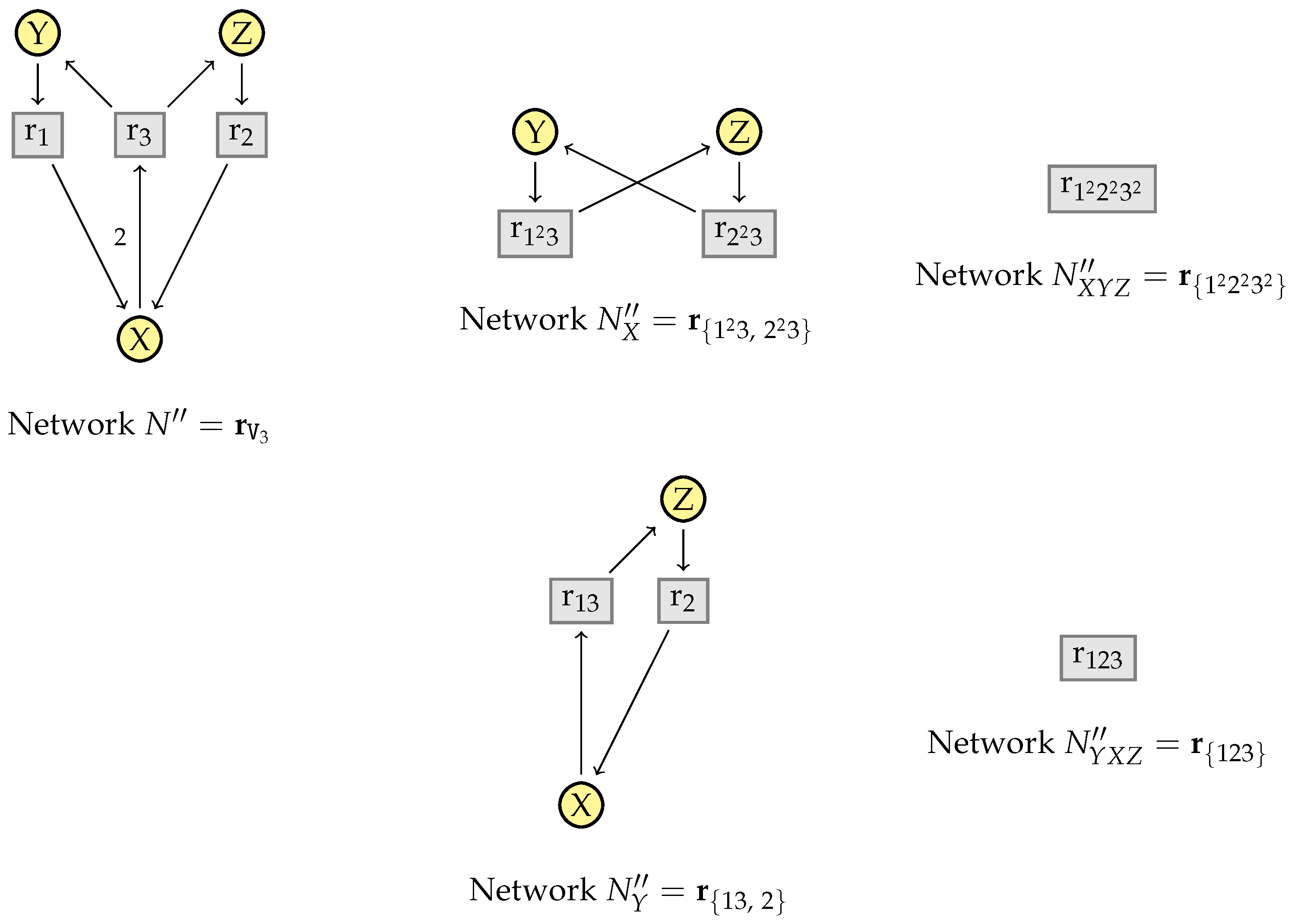
5.3. Factorization
5.4. Proving Confluence via Elementary Modes
- Case
- . Suppose that (F-Fact) replaces vector by vector so that for some . Hence . And thus, , which is equivalent to as required.
- Case
- . By rule (F-Dep) there exist , and such that . If all are distinct from then trivially . Otherwise, we can assume without loss of generality that with v and as in rule (F-Dep). Suppose that these have the forms and . Since , it follows that:This yields . Since this is is equivalent to as required.
- Case
- . Suppose that the intermediate species was eliminated thereby. Recall that . We can assume without loss of generality that for all . Let P, C, , and be as introduced in the Diamond Lemma 3, where , homomorphism h the identity on , and for all . The lemma then yields:Since it follows that . Furthermore, since otherwise so that (F-Inter) could not be applied. Since , this tuple is equal to . With we get:This multiset is an invariant, since . It follows that:This implies . Since and since is closed by factorization with nonzero factors, it follows that as required.
- Case
- . Suppose that (F-Fact) replaces vector by vector so that for some . Since we have . And thus, , which is equivalent to , and thus as required.
- Case
- . By rule (F-Dep) there exist , and such that . If all are distinct from then trivially . Otherwise, we can assume without loss of generality that with v and as in the rule. Suppose that these have the forms and . Since , it follows that:This yields . Since this is is equivalent to as required.
- Case
- . Suppose that the intermediate species was eliminated thereby. We recall that . Without loss of generality, we can assume that all elements of occur exactly once in this sum. Let , , , and . If for and , we note . Otherwise, if with , we note . By the rule (F-Inter) we have:Hence .
6. Reaction Networks with Deterministic Semantics
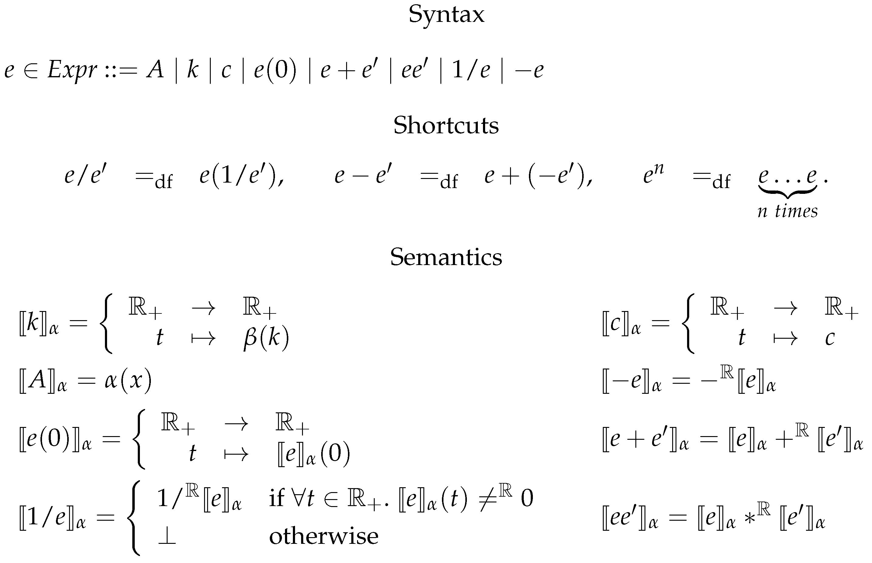
6.1. Kinetic Expressions
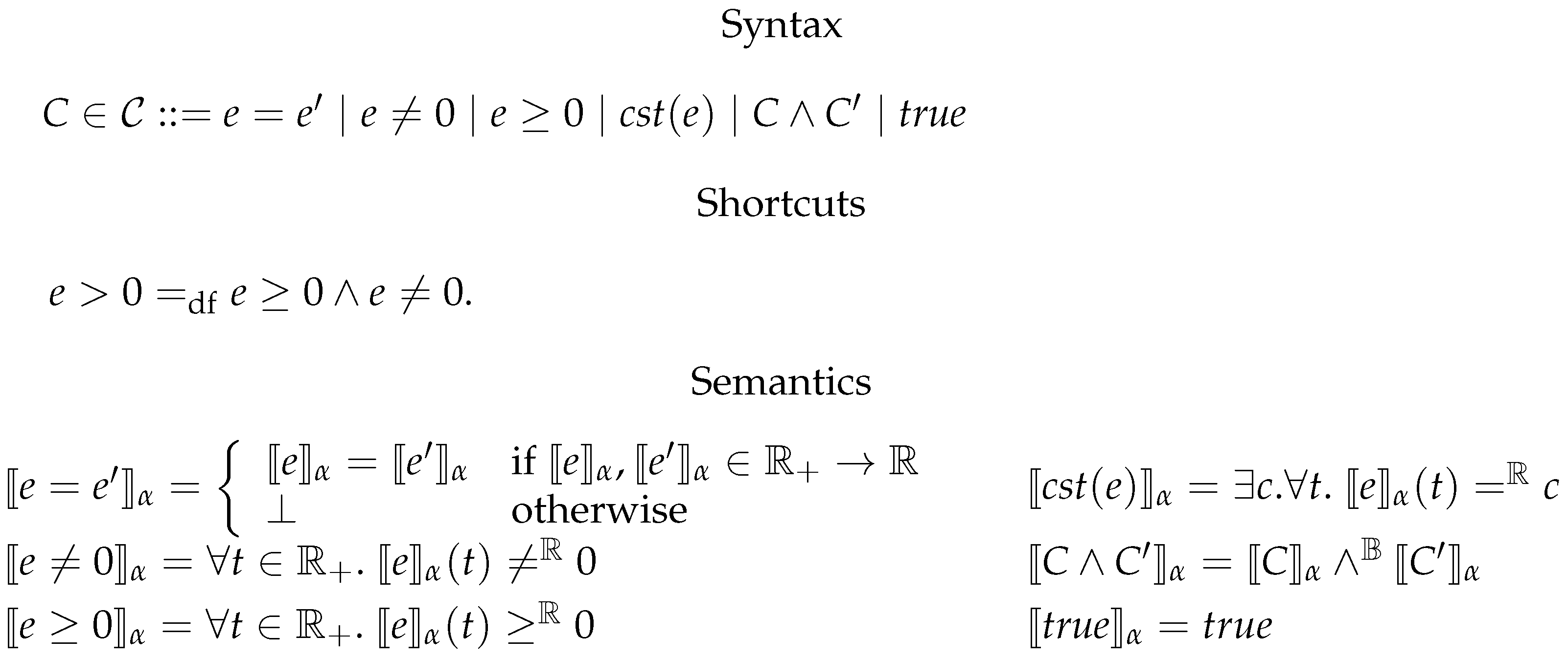
6.2. Constrained Flux Networks
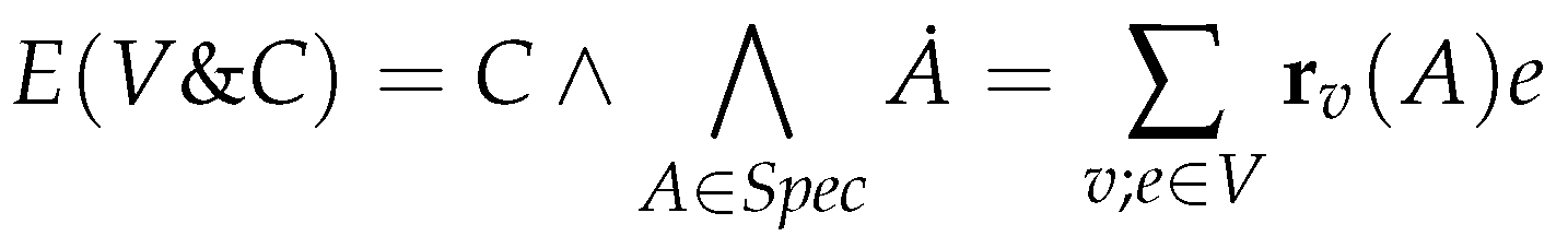
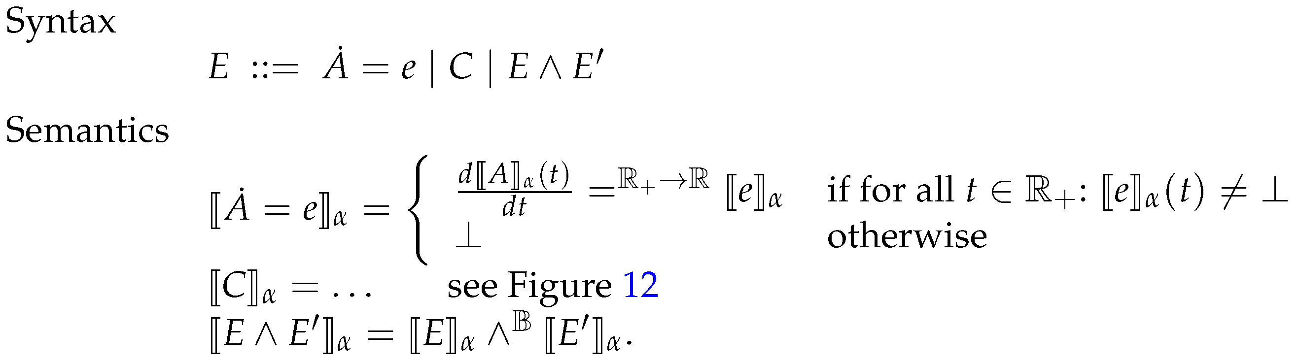
6.3. Systems of Constrained Equations with ODEs
6.4. Deterministic Semantics
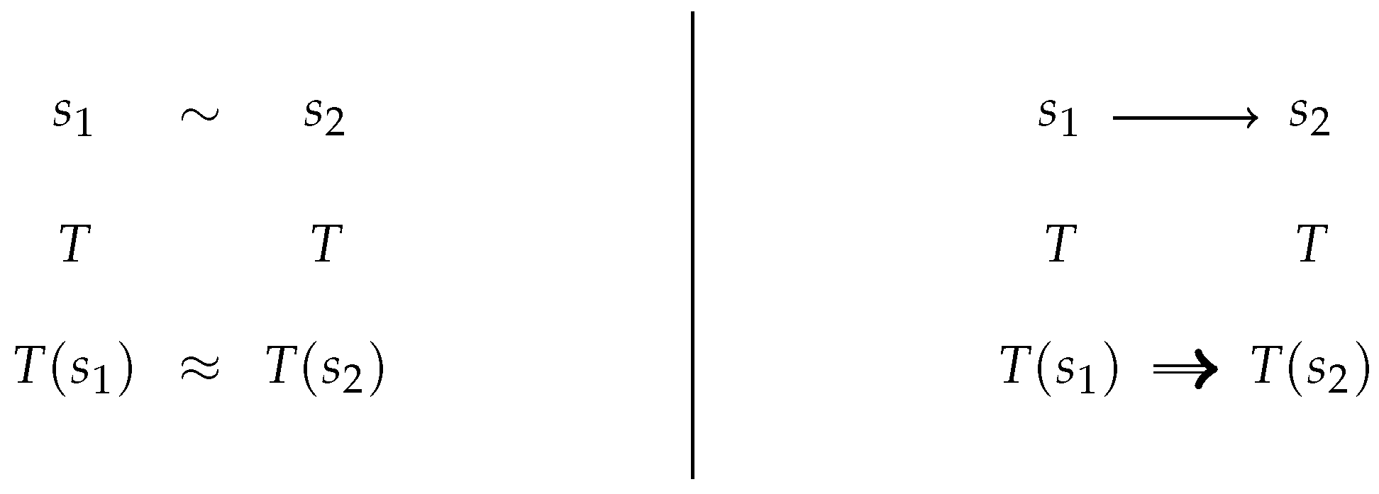
6.5. Contextual Equivalence
7. Simplification of Constrained Flux Networks
7.1. Linear Steadiness of Intermediate Species
- Partial steady state: the concentration of X is steady, i.e., .
- Linear consumption: if a reaction in V consumes X then its kinetic expression is linear in X, that is: if such that then for some expression such that .
- Independent production: if a reaction in V produces X then its kinetic expression does not contain X except for subexpressions : for any , if then .
- Nonzero consumption: the consumption of X is nonzero: .
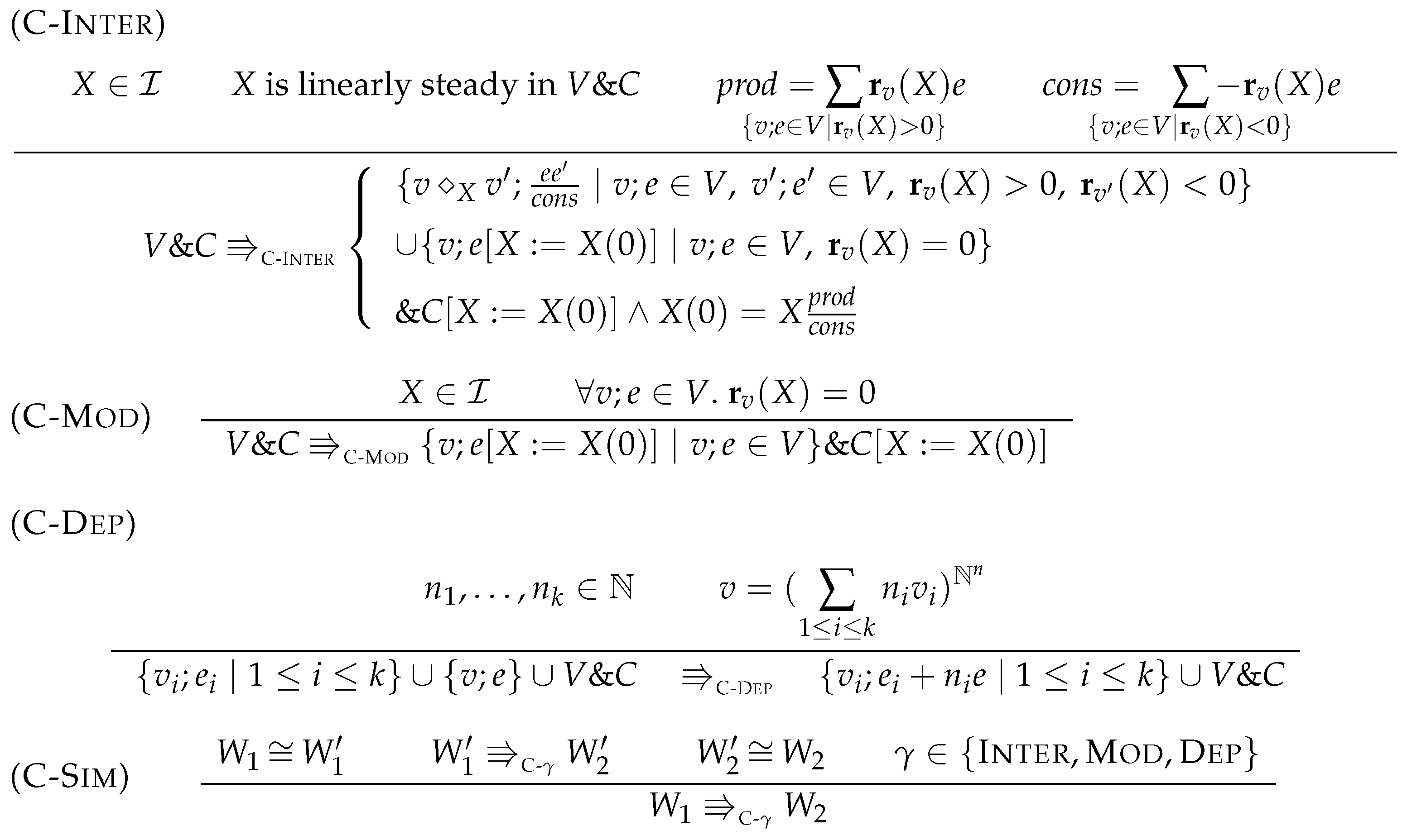
7.2. Simplification
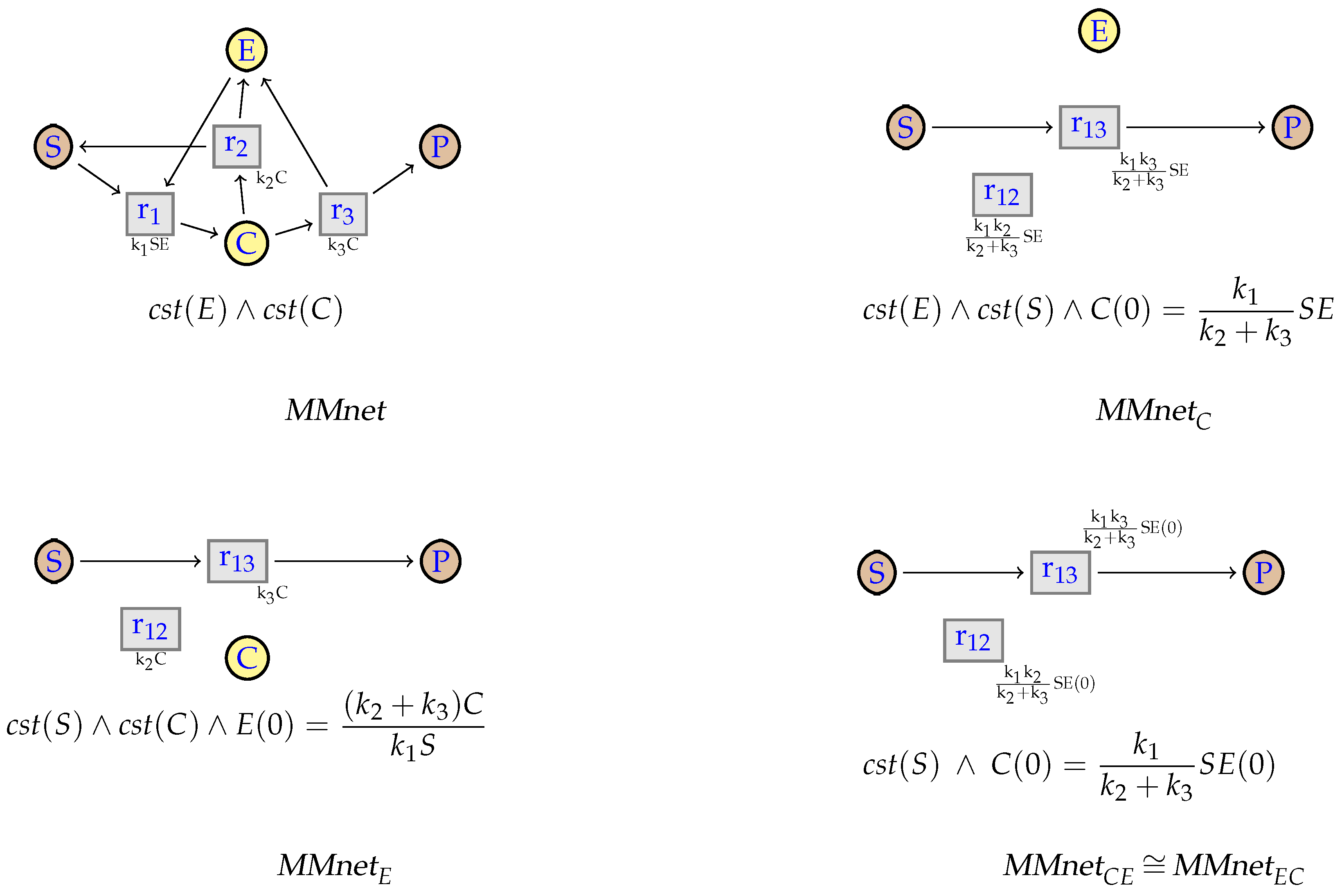
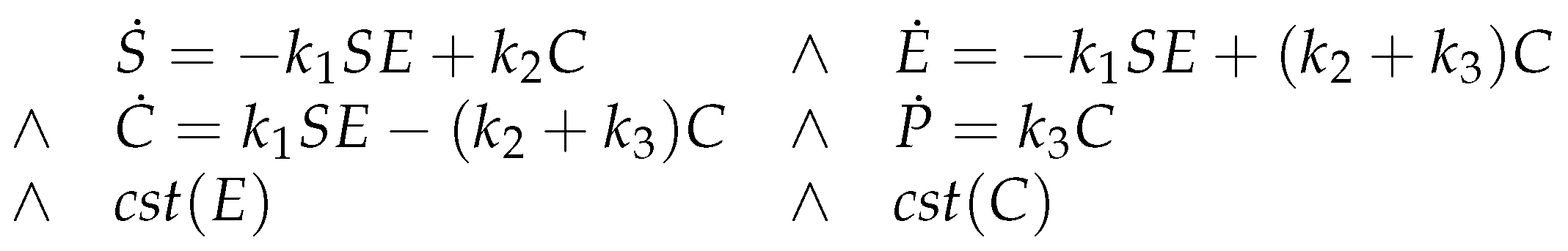
7.3. Michaelis-Menten

8. Preservation of Linear Steadiness
8.1.
- 1.
- Either X is linearly steady in , or X is only a modifier, that is for any we have .
- 2.
- No intermediate species different from X occurs in the kinetic expression of a reaction that consumes X: for any , if , then .
- 3.
- The rate of a reaction that produces X but does not consume an intermediate species does not depend on the concentration of any intermediate species: for any , if and , then .
- 4.
- The total stoichiometry of the intermediate species in the reactant (resp. product) of a reaction is never greater than one: for any , and .
8.2. Stability of
- there exists an index i such that , , and
- for any , .
9. Confluence of the Simplification Relation
9.1. Structural Confluence
9.2. Non-Confluence of the Kinetic Rates
9.3. Criterion for the Full Confluence
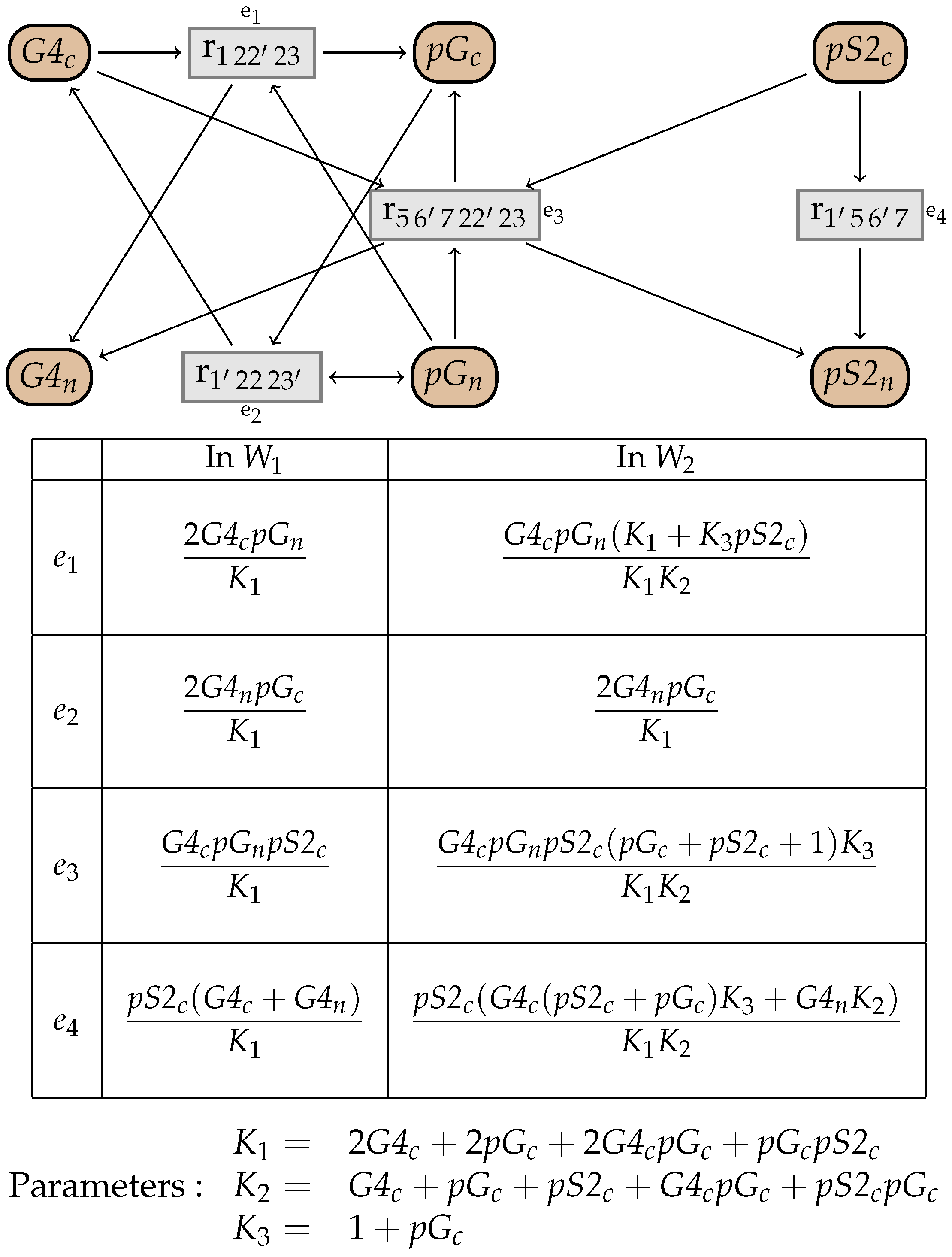
10. An Example from the BioModels Database
11. Simplification of Systems of Equations
11.1. Simplification of Systems of Equations
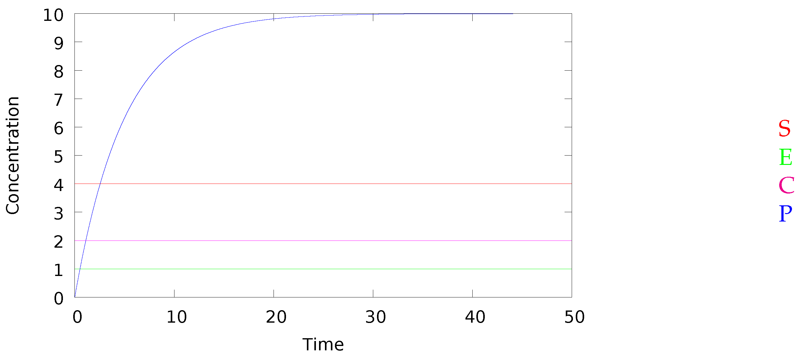
11.2. Simulation
| = | ||
| = | ||
| = | ||
| = | ||
| = | . |
12. Conclusions
Acknowledgments
Author Contributions
Conflicts of Interest
Appendix A. Soundness of the Simplification Rules for Constrained Flux Networks
Appendix B. Proofs for the Stability of LinNets
- a path is a (non empty) sequence of unit vectors , such that for any , we have ;
- we denote the vector of a path by ;
- a path is circular if , and non-circular otherwise;
- for a circular path , we denote the number of intermediate species occurring in the path by ;
- for a non-circular path , we denote its beginning and its end by and . In addition, we define the multiset . Note that we do not count and in this multiset.
- a non-circular flux-path is a non-circular path in W such that for any intermediate species X with , we have (meaning that one of the simplification steps removes X from ), and such that and are either the empty solution ∅, or the intermediate species that are still in W,
- a circular flux-path is a circular path in W if there is at most one intermediate species X such that and (i.e., X is not yet simplified),
- we call flux-path a path that is either a circular or a non-circular flux-path.
- a flux-path is said to correspond to a flux v in W if .
- 1.
- for any flux , there is a corresponding flux-path for W such that . Moreover, if v is not dependent then, for any intermediate species X, we have ;
- 2.
- for any flux-path for W such that for any X, , there is a corresponding flux , that is ;
- 3.
- if depends on , then
- there exists an index i such that , , and
- for any , and any flux-path that corresponds to v is circular.
- (1)
- for flux in the initial network , v is necessarily a unary vector for some i. So we can directly associate the flux-path that trivially corresponds to v. Since it is a unary vector, the flux v is also necessarily not dependent. Because a flux-path of size 1 is always non-circular, we also have, for any intermediate species X, , and thus as required.
- (2)
- any flux-path for is necessarily of size 1. Otherwise, for being a non-circular flux-path, there would exist some . And for being a circular flux-path, there would exist at least two species X and Y such that and , which contradicts the definition of circular flux-path. Then there exists such that .
- (3)
- as said above, a flux v can not be dependent.
- (1)
- Let , then it is the case that for some expression because the rule (C-Dep) only removes a dependent flux and modifies some kinetic expressions. By induction hypothesis, there is a flux-path for such that . Also, because , any flux-path for is also a flux-path for W, which proves that is a flux-path for v. Finally, if v is dependent in W, it is necessarily dependent in W and satisfies by induction hypothesis.
- (2)
- Let be a flux-path for W such that, for any intermediate species X, . Again, because , is also a flux-path for . By induction hypothesis, there is a corresponding flux . If is not the flux that is removed by the application of (C-Dep), then this flux still occurs in W (possibly with an updated kinetic) and we conclude directly. We now show that it can not actually be otherwise, and more precisely, that assuming v removed by (C-Dep) contradicts .Suppose that v is removed by (C-Dep), then v depends on some fluxes in . For the sake of simplicity, we only consider the case where for some intermediate . The other case works similarly. We necessarily have , because contradicts the linearity assumption. By induction hypothesis and Point 3, there exists in particular at least one j such that . Again, by induction hypothesis, there exists a circular flux-path corresponding to in . Since it is circular, there exist some intermediate species such that for any , and , and , . Note that we also have , since, by definition of flux-path, for any i, while . Since and , the unit vectors also appear in the flux-path . So the intermediate species are present at least one time in . Moreover, there is at least one i such that in , the unit vector is preceded by a unit vector that is not one of . Therefore, is produced by another flux, i.e., , which contradicts the hypothesis.
- (3)
- Let be a flux dependent on , that is, in particular, for some . Since (C-Dep) removes one flux and possibly modifies some kinetics, there is a flux in that either depends on or on where is the flux removed by (C-Dep). The latter case is not possible, since it would imply that for some and unary vector . Thus, we conclude that depends on that, by induction hypothesis, satisfies the conditions of Point 3.
- (1)
- Let be in W. Either there is a corresponding flux , and we conclude directly by induction hypothesis, or is the result of merging some that produces X and some that consume it. In this case, by induction hypothesis, there are some corresponding flux-paths and . The concatenation of these paths is a flux-path. Indeed,
- the production of coincides with the consumption of because there is an intermediate species X such that , and .
- if is non-circular, for any intermediate species Y such that , either and , or, or and by induction hypothesis, that is .
- if is circular, there exists an intermediate species Y which is both consumed by and produced by . The flux-path cannot be circular, as this would imply , and similarly for . By definition of non-circular flux-path, X and Y are the only two species in and such that and . Thus, Y is the only non-eliminated intermediate species in w.r.t. W, meaning again that is indeed a circular flux-path.
Moreover, trivially corresponds to v. We prove with Point 3 that if is non-dependent, then for any X. - (2)
- Let be a flux-path for W such that for any Y, . Let X be the intermediate species removed by (C-Inter), in particular , hence either or . Since , if , then is also a flux-path for , so by induction there is a corresponding flux . Since , we still have a flux , that corresponds to . If then we can decompose into producing X and consuming X such that . and can not be circular, as this would imply that X is both consumed and produced by and by , contradicting the fact that . Therefore . Again, because and X is the species removed by (C-Inter) and is a flux-path, and are (non-circular) flux-paths for . We can then apply the induction hypothesis and infer that there are some corresponding fluxes , the first one that produces X and the second one that consumes it. Consequently, there is a flux that is the merging of and , and that corresponds to .
- (3)
- Let be a flux that depends on and X be the intermediate species removed by (C-Inter). We distinguish two cases: either (case 1) is the simplification of some flux (meaning that v does neither produce nor consume X) or (case 2) it results from merging fluxes that produce and consume X.(Case 1) By induction hypothesis and Point 1, there exists a flux-path corresponding to v for . We have since X has not been removed. Suppose that there is such that is the merging, by (C-Inter), of fluxes that produce and a consume X. In this case, for any corresponding to , and, by the Lemma A1, we would have that , which contradicts . Therefore, none of the s are the merging of other fluxes by (C-Inter), therefore, there are such that depends on those fluxes. Since, by induction hypothesis, Point 3 is satisfied for in , it is also satisfied for in W.(Case 2) Let be a flux that produces X, and a flux that consumes it and their merging. Let and be flux-paths in for, respectively, and (such flux paths exist by induction hypothesis). Any corresponding path is then the concatenation of corresponding paths and .We first prove that, if either or is dependent in , then is also dependent in W. By induction, if depends on , there exists a unique i such that , , and, for any , . Then, there is a flux in W that is the merging of and , and there are fluxes in W for . Then depends on and the .If both and are not dependent, by induction hypothesis, for any , in the corresponding flux-path, we have and . If , then . We also have (indeed, X is the removed species, so and the X produced by is merged with the X consumed by in ). Therefore, in this case Point 1 is satisfied. If there is a Y such that , then Y occurs twice in , and there is an intermediate species Z (that can possibly be Y if no other intermediate species occurs more than once between both occurrences of Y) such that and such that there is a circular flux-path , subpath of that begins and end with Z:
![Computation 05 00014 i002]() Then using Point 2, there is a corresponding flux , with . We can repeat the same operation on the remaining path , and obtain at each step a new (circular) flux. We stop when we obtain a remaining path , such that for any Y, we have . Then there is a corresponding flux with , and . Then v is dependent on and the set of circular fluxes we obtained in this process. Therefore, in this case Point 3 is satisfied.Now assume that and are dependent, and so that is dependent too. By induction and using Point 3, depends on a flux with and , and on other fluxes such that , and similarly for . Then any and any is still in W, while is merged with , forming a new flux . Then depends on , the and the . Since , and similarly , Point 3 is satisfied.
Then using Point 2, there is a corresponding flux , with . We can repeat the same operation on the remaining path , and obtain at each step a new (circular) flux. We stop when we obtain a remaining path , such that for any Y, we have . Then there is a corresponding flux with , and . Then v is dependent on and the set of circular fluxes we obtained in this process. Therefore, in this case Point 3 is satisfied.Now assume that and are dependent, and so that is dependent too. By induction and using Point 3, depends on a flux with and , and on other fluxes such that , and similarly for . Then any and any is still in W, while is merged with , forming a new flux . Then depends on , the and the . Since , and similarly , Point 3 is satisfied.

Appendix C. Proofs of the Full Confluence of the Simplification
- the combination of and the consuming fluxes: ,
- the combination of and the consuming reactions: ,
- the other combined fluxes: ,
- the remaining fluxes not combined: ,
- the other fluxes that are not in , , , where we substitute X by .
- ,
- ,
- ,
- the other fluxes that are not in , , , where we substitute X by .
- ,
- ,
- the other fluxes that are not in , , .
- ,
- ,
- ,
- the other fluxes that are not in , , , where we substitute X by .
- , the fluxes producing X without Y,
- , the fluxes consuming X without Y,
- , the fluxes with modifier X and without Y,
- , the fluxes producing Y without X,
- , the fluxes consuming Y without X,
- , the fluxes with modifier Y and without X,
- , the fluxes producing X and consuming Y,
- , the fluxes producing Y and consuming X,
- , the fluxes with modifier X and Y.
- ,
- ,
- ,
- .
- ,
- .
- ,
- ,
- .
- .
- ,
- ,
- .
- ,
- ,
- ,
- .
- ,
- ,
- ,
- .
- ,
- ,
- ,
- ,
- ,
- ,
- ,
- ,
- the 2 first sets are symmetric to each other, in the sense that if we switch X and Y in the first set, we obtain the second one,
- the 2 following sets are symmetric to each other,
- the 2 following sets are symmetric to each other too,
- the following set is symmetric in X and Y,
- the last set is symmetric in X and Y (since the substitutions commute).
References
- Feinberg, M. Chemical reaction network structure and the stability of complex isothermal reactors—I. The deficiency zero and deficiency one theorems. Chem. Eng. Sci. 1987, 42, 2229–2268. [Google Scholar] [CrossRef]
- Hucka, M.; Finney, A.; Sauro, H.M.; Bolouri, H.; Doyle, J.C.; Kitano, H.; Arkin, A.P.; Bornstein, B.J.; Bray, D.; Cornish-Bowden, A.; et al. The systems biology markup language (SBML): A medium for representation and exchange of biochemical network models. Bioinformatics 2003, 19, 524–531. [Google Scholar] [CrossRef] [PubMed]
- Calzone, L.; Fages, F.; Soliman, S. BIOCHAM: An environment for modeling biological systems and formalizing experimental knowledge. Bioinformatics 2006, 22, 1805–1807. [Google Scholar] [CrossRef] [PubMed]
- Kuttler, C.; Lhoussaine, C.; Nebut, M. Rule-based modeling of transcriptional attenuation at the tryptophan operon. In Transactions on Computational Systems Biology XII; Springer: New York, NY, USA, 2010; pp. 199–228. [Google Scholar]
- Chaouiya, C. Petri net modelling of biological networks. Brief. Bioinform. 2007, 8, 210–219. [Google Scholar] [CrossRef] [PubMed]
- Juty, N.; Ali, R.; Glont, M.; Keating, S.; Rodriguez, N.; Swat, M.J.; Wimalaratne, S.M.; Hermjakob, H.; Le Novère, N.; Laibe, C.; et al. BioModels: Content, Features, Functionality and Use. CPT Pharmacomet. Syst. Pharmacol. 2015, 4, 55–68. [Google Scholar] [CrossRef] [PubMed]
- Mäder, U.; Schmeisky, A.G.; Flórez, L.A.; Stülke, J. SubtiWiki—A comprehensive community resource for the model organism Bacillus subtilis. Nucleic Acids Res. 2012, 40, 1278–1287. [Google Scholar] [CrossRef] [PubMed]
- Niehren, J.; John, M.; Versari, C.; Coutte, F.; Jacques, P. Qualitative Reasoning about Reaction Networks with Partial Kinetic Information. In Computational Methods for Systems Biology; Lecture Notes in Computer Science; Springer: New York, NY, USA, 2015; Volume 9308, pp. 157–169. [Google Scholar]
- Radulescu, O.; Gorban, A.N.; Zinovyev, A.; Noel, V. Reduction of dynamical biochemical reactions networks in computational biology. Front. Genet. 2012, 3, 131. [Google Scholar] [CrossRef] [PubMed]
- Michaelis, L.; Menten, M.L. Die kinetik der invertinwirkung. Biochem. Z. 1913, 49, 333–369. (In German) [Google Scholar]
- Segel, L.A. On the validity of the steady state assumption of enzyme kinetics. Bull. Math. Biol. 1988, 50, 579–593. [Google Scholar] [CrossRef] [PubMed]
- Cornish-Bowden, A. Fundamentals of Enzyme Kinetics; Wiley: Hoboken, NJ, USA, 2013. [Google Scholar]
- Heineken, F.; Tsuchiya, H.; Aris, R. On the mathematical status of the pseudo-steady state hypothesis of biochemical kinetics. Math. Biosci. 1967, 1, 95–113. [Google Scholar] [CrossRef]
- Segel, L.A.; Slemrod, M. The quasi-steady-state assumption: A case study in perturbation. SIAM Rev. 1989, 31, 446–477. [Google Scholar] [CrossRef]
- King, E.L.; Altman, C. A schematic method of deriving the rate laws for enzyme-catalyzed reactions. J. Phys. Chem. 1956, 60, 1375–1378. [Google Scholar] [CrossRef] [Green Version]
- Chou, K.-C.; Forsen, S. Graphical rules of steady-state reaction systems. Can. J. Chem. 1981, 59, 737–755. [Google Scholar]
- Fages, F.; Gay, S.; Soliman, S. Inferring reaction systems from ordinary differential equations. Theor. Comput. Sci. 2015, 599, 64–78. [Google Scholar] [CrossRef]
- Sáez, M.; Wiuf, C.; Feliu, E. Graphical reduction of reaction networks by linear elimination of species. J. Math. Biol. 2017, 74, 195–237. [Google Scholar] [CrossRef] [PubMed]
- Madelaine, G.; Lhoussaine, C.; Niehren, J. Attractor Equivalence: An Observational Semantics for Reaction Networks. In Formal Methods in Macro-Biology; Springer: New York, NY, USA, 2014. [Google Scholar]
- Schmidt-Schauss, M.; Sabel, D.; Niehren, J.; Schwinghammer, J. Observational Program Calculi and the Correctness of Translations. J. Theor. Comput. Sci. 2015, 577, 98–124. [Google Scholar] [CrossRef]
- Gagneur, J.; Klamt, S. Computation of elementary modes: A unifying framework and the new binary approach. BMC Bioinform. 2004, 5, 175. [Google Scholar] [CrossRef] [PubMed] [Green Version]
- Madelaine, G.; Lhoussaine, C.; Niehren, J.; Tonello, E. Structural simplification of chemical reaction networks in partial steady states. Biosystems 2016, 149, 34–49. [Google Scholar] [CrossRef] [PubMed]
- Schmierer, B.; Tournier, A.L.; Bates, P.A.; Hill, C.S. Mathematical modeling identifies Smad nucleocytoplasmic shuttling as a dynamic signal-interpreting system. Proc. Natl. Acad. Sci. USA 2008, 105, 6608–6613. [Google Scholar] [CrossRef] [PubMed]


© 2017 by the authors. Licensee MDPI, Basel, Switzerland. This article is an open access article distributed under the terms and conditions of the Creative Commons Attribution (CC BY) license ( http://creativecommons.org/licenses/by/4.0/).
Share and Cite
Madelaine, G.; Tonello, E.; Lhoussaine, C.; Niehren, J. Simplification of Reaction Networks, Confluence and Elementary Modes. Computation 2017, 5, 14. https://doi.org/10.3390/computation5010014
Madelaine G, Tonello E, Lhoussaine C, Niehren J. Simplification of Reaction Networks, Confluence and Elementary Modes. Computation. 2017; 5(1):14. https://doi.org/10.3390/computation5010014
Chicago/Turabian StyleMadelaine, Guillaume, Elisa Tonello, Cédric Lhoussaine, and Joachim Niehren. 2017. "Simplification of Reaction Networks, Confluence and Elementary Modes" Computation 5, no. 1: 14. https://doi.org/10.3390/computation5010014