An Accurate Computational Tool for Performance Estimation of FSO Communication Links over Weak to Strong Atmospheric Turbulent Channels

Abstract

The terrestrial optical wireless communication links have attracted significant research and commercial worldwide interest over the last few years due to the fact that they offer very high and secure data rate transmission with relatively low installation and operational costs, and without need of licensing. However, since the propagation path of the information signal, i.e., the laser beam, is the atmosphere, their effectivity affects the atmospheric conditions strongly in the specific area. Thus, system performance depends significantly on the rain, the fog, the hail, the atmospheric turbulence, etc. Due to the influence of these effects, it is necessary to study, theoretically and numerically, very carefully before the installation of such a communication system. In this work, we present exactly and accurately approximate mathematical expressions for the estimation of the average capacity and the outage probability performance metrics, as functions of the link’s parameters, the transmitted power, the attenuation due to the fog, the ambient noise and the atmospheric turbulence phenomenon. The latter causes the scintillation effect, which results in random and fast fluctuations of the irradiance at the receiver’s end. These fluctuations can be studied accurately with statistical methods. Thus, in this work, we use either the lognormal or the gamma–gamma distribution for weak or moderate to strong turbulence conditions, respectively. Moreover, using the derived mathematical expressions, we design, accomplish and present a computational tool for the estimation of these systems’ performances, while also taking into account the parameter of the link and the atmospheric conditions. Furthermore, in order to increase the accuracy of the presented tool, for the cases where the obtained analytical mathematical expressions are complex, the performance results are verified with the numerical estimation of the appropriate integrals. Finally, using the derived mathematical expression and the presented computational tool, we present the corresponding numerical results, using common parameter values for realistic terrestrial free space optical communication systems.

1. Introduction

The optical wireless—or free space optical (FSO)—communication systems offer high bandwidth and secure access along with low installation and maintenance cost without needing any operational license. Thus, this technology attracts very significant research of experimental and commercial interest, especially in the last few years [1,2,3,4,5,6,7,8]. However, the performance and the availability of terrestrial FSO links depends strongly on the atmospheric conditions in the area where the link is installed. More specifically, the fog, the rain, the hail, etc. affect significantly their effectivity, while another very significant phenomenon for the availability and performance decreasing is the atmospheric turbulence which causes the scintillation effect that induces rapid fluctuations of the optical signal on the receiver’s side. Thus, the FSO channels have randomly time-varying characteristics due to the scintillation effect [9,10,11,12]. In order to study these signal’s fluctuations, many statistical models have been proposed and tested experimentally for various atmospheric turbulence conditions. More specifically, for the case of strong to very strong turbulence conditions, the K-distribution model is usually used, for saturated turbulence, the negative exponential statistical distribution, and, for weak turbulence, the lognormal, the gamma, the Malaga and the Rayleigh distributions can be used, while, for moderate to strong cases, the gamma–gamma, the Malaga and the I-K models are used [12,13,14,15,16,17,18,19,20,21,22,23,24,25,26,27,28,29,30,31,32]. In this work, we use either the lognormal distribution model, which is accurate enough for the cases of weak turbulence conditions, or the gamma–gamma which is the suitable statistical distribution to model the irradiance fluctuations at the receiver for the cases of moderate to strong turbulence [13,14,17,18,27,28,29,30,31,32].

In this work, taking into account the fog and atmospheric turbulence, the performance and the availability of the FSO links are estimated by means of the average capacity and outage probability metrics [13,27,28,29]. Thus, we derive either closed form mathematical expressions or accurate approximate ones, for the evaluation of these metrics as functions of the transmitted power, the attenuation due to the fog, the atmospheric turbulence and the link’s parameters. The obtained expression are using either the lognormal distribution, for the cases where the turbulence strength can be assumed as weak, or the gamma–gamma for moderate to strong turbulence.

Next, using the derived mathematical expressions, we design, implement and present a new mathematical tool that evaluates accurately these two abovementioned performance quantities, using as input realistic parameters for the link, the fog attenuation, the transmitted power and the strength of the atmospheric turbulence effect. The computational tool, through the proposed algorithm, estimates the system’s performance and availability by means of the derived expression for the average capacity and the outage probability, respectively. Furthermore, due to the complexity of the derived mathematical expressions that are using the gamma–gamma distribution model, the algorithm re-evaluates the metric value without using the derived analytical expression but with the computational estimation of the corresponding integrals, in order to verify the results and the validity of the analytical predictions [33]. Moreover, it should be mentioned that, in the future, the influences of other effect, e.g., rain, hail, etc., can be added. However, due to the operational wavelength of the FSO links, the fog and the turbulence effects play very significant roles in their performance, and, for this reason, we study them theoretically and computationally in this work [33].

The work presented in this manuscript is organized as follows: in Section 2, we introduce the FSO system, the channel model, the link parameters, the fog attenuation, the atmospheric turbulence effect, the lognormal and the gamma distributions. Next, in Section 3, we present the performance metrics for the FSO communication link and we derive the mathematical expressions for the estimation of the outage probability and the average capacity. In Section 4, we present the algorithm structure for the computational tool, while, in Section 5, we present the numerical results for common realistic FSO configurations. In Section 6, the final conclusions are presented and the Appendix A with the pseudo-code algorithm follows.

2. Channel Model

We consider a point-to-point terrestrial FSO link, with additive white Gaussian noise (AWGN), in which the information signal, i.e., the laser beam, propagates along a horizontal path. The channel can be assumed that is stationary and ergodic and the statistical channel model is given as [29]:

$$y=\eta {\rm I} x+n,$$

(1)

where y is the received signal, x is the modulated signal, i.e., takes the values “0” or “1”, η is the detector’s responsitivity, n is the AWGN with zero mean value and variance N₀/2, whereas I is the normalized instantaneous irradiance on the receiver’s side [20].

As mentioned above, the atmospheric turbulence effect affects significantly the performance of an FSO link due to the scintillation effect, which results in fast and large irradiance fluctuations on the receiver’s end. Taking into account the atmospheric turbulence strength, the operational wavelength of the communication system and the link’s length, the Rytov variance can be estimated, which is a parameter that measures the severity of intensity scintillation caused by the distributed atmospheric turbulence, i.e., the strength of the turbulence effect [34]. More specifically, the Rytov variance, ${\sigma }_l^2$, is given as [29,35]:

$${\sigma }_l^2=1.23C_n^2{k}^{\raisebox{1ex}{$7$}\!\left/ \!\raisebox{-1ex}{$6$}\right.}{L}^{\raisebox{1ex}{$11$}\!\left/ \!\raisebox{-1ex}{$6$}\right.},$$

(2)

where $k=2\pi /\lambda$ is the wave number, λ is the wavelength, L stands for the link length and $C_n^2$ represents the refractive index structure parameter, and it is proportional to the atmospheric turbulence strength [36]. The Rytov variance represents the normalized irradiance variance or the scintillation index and characterizes the turbulence strength as follows [3,37]:

$$\begin{array}{ccc}{\sigma }_l^2\le 0.3& & (\text{weak fluctuations})\\ 0.3<{\sigma }_l^2<5& & (\text{moderate to strong fluctuations})\\ {\sigma }_l^2>>1& & (\text{saturation fluctuations})\end{array}.$$

(3)

Taking into account that the irradiance fluctuations at the receiver of the FSO link, due to the scintillation effect, are studied with statistical models, and the main criterion for their choice is the atmospheric turbulence strength, the regions that appear in Equation (3) can be used. Thus, in this work, for the case of weak turbulence conditions, i.e., ${\sigma }_l^2\le 0.3$, the lognormal distribution model is used, while for values larger than 0.3 and up to 5, the turbulence strength can be assumed as moderate to strong and the gamma–gamma distribution is suitable.

The irradiance fluctuations at the receiver results in fluctuations in the dependent quantities. More specifically, the instantaneous electrical signal-to-noise ratio (SNR) at the receiver, γ, behaves as a random variable and is given as [36]:

$$\gamma =\frac{{\left(\eta {\rm I}{P}_r\right)}^2}{N_0},$$

(4)

while the expected electrical SNR on the receiver’s side, μ, is given as [29,31]:

$$\mu =\frac{{\left(\eta {\rm E}\left[{\rm I}\right]P_r\right)}^2}{N_0},$$

(5)

where P_r is the expected signal power at the receiver while N₀ is given as [32,38,39]:

$$N_0=\frac{4{{\rm K}}_{{\rm B}}{{\rm T}}_{abs}B{F}_n}{R_L}+2q_{e}B\left(I_{ph}+I_D\right)+\left(RIN\right){I_{ph}}^2,$$

(6)

with K_B being the Boltzmann constant, T_abs being the absolute system temperature, F_n is the photodiode noise figure, R_L the load resistor [36], I_D, is the dark current on photodetector [40], RIN the relative intensity noise process and a typical value is −130 dB/Hz, and $q_e$ is the electron charge, whereas $I_{ph}=P_r\eta$ is the average receiver photocurrent [31].

Furthermore, it should be mentioned here that another significant performance mitigation factor of the FSO link, is the background, or the ambient noise, and is caused by the background radiation, which is collected by the lens of the receiver of the optical system in addition to the information signal [4,41,42,43,44,45]. In order to decrease its influence, optical filters of bandwidth B_f, before the receiver’s lens are usually used [45]. Thus, assuming that the background noise is Gaussian with spectral density N_b, the total power of the ambient noise, which arrives at the receiver’s input, is B_fN_b. The influence of the ambient noise at the total system’s noise is given through [45] and Equation (6) and has the mathematical form:

$$N_0=\frac{4{{\rm K}}_{{\rm B}}{{\rm T}}_{abs}B{F}_n}{R_L}+2q_{e}B\left(I_{ph}+I_D\right)+2B{\eta }^2{N}_b^2{B}_f/r+\left(RIN\right){I_{ph}}^2,$$

(7)

where $r={\omega }_{FOV}/{\omega }_D$, ${\omega }_{FOV}$ represents the receiver’s field of view while ${\omega }_D$ stands for the solid angle subtended by the background source at the receiver [45].

For the estimation of the expected signal at the receiver’s side, P_r, taking into account the visibility at the area of the FSO link and losses due to the scintillation effect, using [2,33,46,47], we make a conclusion of the following expression:

$$P_r=P_T G_T{G}_R{\left(\frac{\lambda }{4\pi L}\right)}^2{\left(\frac{D_R}{D_T+\mathsf{\theta }L}\right)}^2{10}^{-\left(L{a}_{tot}+L_m\right)/10},$$

(8)

where $P_T$ is the transmitted power,$G_T$, $G_R$ are the gains of transmitter and receiver, respectively, which are computed from initial parameters [33], D_R and D_T are the transmitter’s and receiver’s aperture, $\theta$ stands for the beam’s divergence, a_tot, represents the atmospheric attenuation that includes the fog phenomenon, a_f, the rain, a_r, the snow a_sn, and the scintillation effect, a_s, which affect significantly the performance of the FSO links while $L_m$, stands for the miscellaneous losses of the system, as it is presented in [2,4,33,46,47]. More specifically, the attenuation parameter due to the fog is given through the Kim or the Kruse model depending on the effect’s strength, and the atmospheric visibility V with sky droplets are set to τ_TH = 5% [47]. Furthermore, the scintillation losses parameter in dB is given as: $a_s=\sqrt{92.68\cdot {\left(2\pi {10}^9/\lambda \right)}^{7/6}{C}_n^2{L}^{11/6}}$ [47].

All of the above parameters are taken into account by our tool and some common values are presented in

Table 1. The common parameter values of an FSO communication link.

Parameter	Symbol	Value
Transmitted Power	PT	400 mW (26 dBm)
Wavelength	λ	1550 nm
Transmitted Aperture Diameter	DT	2 mm
Beam Divergence	θ (theta)	1 mrad
Miscellaneous Losses	Lm	1 dB
Bandwidth	B	0.5 Ghz
Receiver Aperture	DR	180 mm
Receiver Sensitivity	S (threshold)	−30 or −40 dBm
Sky Droplets	τTH	5%
Detector Responsitivity	η	0.8 A/W
Boltzmann Constant	KB	1.38 × 10−23
Electron Charge Constant	qe	1.602 × 10−19 Cb
Relative Intensity Noise	RIN	−130 dB/Hz
Receiver Noise Figure	Fn	1 (0 dB)
Dark Current	ID	6 nA
Load Resistor	RL	50 Ω
Temperature	Tabs	288 K
Visibility	V	20 km

. Thus, for the specific case, for negligible ambient noise using the suitable infrared filters [48], from Equations (5)–(8), the average electrical SNR at the receiver, as a function of the transmitted power, is given as:

$$\mu =\frac{{\left(\eta P_T G_T{G}_R{\left(\frac{\lambda }{4\pi L}\right)}^2{\left(\frac{D_R}{D_T+\theta \cdot L}\right)}^2{10}^{-\left(L\cdot a_{tot}+L_m\right)/10}\right)}^2}{\left(4{{\rm K}}_{{\rm B}}{{\rm T}}_{abs}B{F}_n/R_L\right)+2q_{e}B\left(I_{ph}+I_D\right)+\left(RIN\right){I_{ph}}^2},$$

(9)

while, for the case where the ambient noise cannot be assumed as negligible, from Equations (5), (6) and (8), the average electrical SNR is given as:

$$\mu =\frac{{\left(\eta P_T G_T{G}_R{\left(\frac{\lambda }{4\pi L}\right)}^2{\left(\frac{D_R}{D_T+\theta \cdot L}\right)}^2{10}^{-\left(L\cdot a_{tot}+L_m\right)/10}\right)}^2}{\left(4{{\rm K}}_{{\rm B}}{{\rm T}}_{abs}B{F}_n/R_L\right)+2q_{e}B\left(I_{ph}+I_D\right)+2B{\eta }^2{N}_b^2{B}_f/r+\left(RIN\right){I_{ph}}^2}.$$

(10)

It should be mentioned here that, although the ambient noise represents a major interference source, especially in daytime hours, its influence can be minimized using specific infrared filters in front of the receiver’s lens for common realistic FSO links [48]. Thus, for the computational tool that we present below, the influence of the ambient noise is considered negligible.

2.1. Lognormal Turbulence Model

The lognormal distribution is a suitable distribution model in order to emulate the irradiance fluctuations at the receiver’s side due to the scintillation effect for the cases of weak turbulence conditions. The corresponding PDF for γ is given as [9,29]:

$$f_{\mathsf{\gamma }}\left(\gamma \right)=\left[\frac{1}{2\gamma \sigma \sqrt{2\pi }}exp\left(-\frac{{\left(\ln \left(\gamma /\mu \right)+{\sigma }^2\right)}^2}{8{\sigma }^2}\right)\right],$$

(11)

where ${\sigma }^2$ is the variance for planar wave of the lognormal distribution that depends on the channel’s characteristics and is given as [3,27,29]:

$${\sigma }^2=\exp \left[\frac{0.49{\sigma }_l^2}{{\left(1+0.65d^2+1.11{\sigma }_l^{12/5}\right)}^{7/6}}+\frac{0.51{\sigma }_n^2{\left(1+0.69{\sigma }_l^{12/5}\right)}^{-5/6}}{{\left(1+0.9d^2+0.62d^2{\sigma }_l^{12/5}\right)}^{5/6}}\right]-1,$$

(12)

where $d=0.5D_R\sqrt{k/L}$ [29].

2.2. Gamma–Gamma Turbulence Model

Another very significant statistical distribution model, for the research area of the FSO link is the gamma–gamma, which has been proven to be very accurate at describing the irradiance fluctuations due to the scintillation effect for the cases of moderate to strong turbulence channels [14,17,31,35]. Its PDF, as a function of γ is given as [17,36]:

$$f_{\gamma }\left(\gamma \right)=\frac{{\left(ab\right)}^{\left(a+b\right)/2}}{\Gamma \left(a\right)\Gamma \left(b\right)}\frac{{\gamma }^{\left(a+b\right)/4-1}}{{\mu }^{\left(a+b\right)/4}}{K}_{a-b}\left(2\sqrt{ab\sqrt{\frac{\gamma }{\mu }}}\right),$$

(13)

where Γ(.) represents the gamma function, K_v is the modified Bessel function of the second kind of order v, and a, b are parameters which can be defined from the link’s parameters and given through the expressions [35,39]:

$$\begin{gathered} a={\left[\exp \left(\frac{0.49{\sigma }_l^2}{{\left(1+0.65d^2+1.11{\sigma }_l^{12/5}\right)}^{7/6}}\right)-1\right]}^{-1}, \\ b={\left[\exp \left(\frac{0.51{\sigma }_l^2{\left(1+0.69{\sigma }_l^{12/5}\right)}^{-5/6}}{{\left(1+0.9d^2+0.62d^2{\sigma }_l^{12/5}\right)}^{5/6}}\right)-1\right]}^{-1}. \end{gathered}$$

(14)

3. Performance of the FSO System

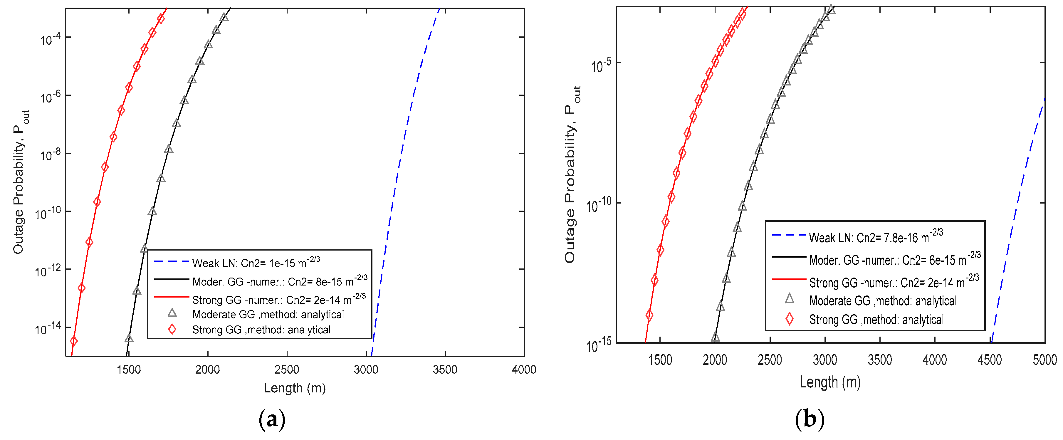
3.1. Outage Probability of the System

A very significant metric for the estimation of the availability of the optical communication system is the outage probability, P_out. More specifically, this quantity represents the probability of the instantaneous SNR to fall below a critical threshold, γ_th, which is set by the receiver’s sensitivity limit [9,27,29,30]:

$$P_{out}=P_r\left(\gamma \le {\mathsf{\gamma }}_{\mathrm{th}}\right)={\displaystyle \underset{0}{\overset{{\gamma }_{th}}{\int }}}{f}_{\gamma }\left(\gamma \right)d\gamma .$$

(15)

From Equation (15) and using the expressions (10)–(12), we reach a conclusion of the following closed form mathematical expression for the estimation of the outage probability of the FSO link through the lognormal distribution model, as a function of the transmitted power and the attenuation parameters due to the fog and the scintillation effect:

$$P_{out}=\frac{1}{2}erfc\left(\frac{1}{2\sqrt{2}\sigma }\left[\ln \left(\frac{{\left(\eta P_T G_T{G}_R{\left(\frac{\lambda }{4\pi L}\right)}^2{\left(\frac{D_R}{D_T+\theta L}\right)}^2{10}^{-\left(L\cdot a_{tot}+L_m\right)/10}\right)}^2}{{\gamma }_{th}\left[\left(4{{\rm K}}_{{\rm B}}{{\rm T}}_{abs}B{F}_n/R_L\right)+2q_{e}B\left(I_{ph}+I_D\right)+2B{\eta }^2{N}_b^2{B}_f/r+\left(RIN\right){I_{ph}}^2\right]}\right)-{\sigma }^2\right]\right).$$

(16)

Similarly as above, from Equation (15) and using the expressions (10), (13) and (14), the following closed mathematical expression is derived for the outage probability estimation of the FSO link, as a function of the transmitted power and the attenuation parameters due to the fog and the scintillation effect using the gamma-gamma distribution model:

$$\begin{array}{l}{P}_{\mathrm{out}}\\ =\frac{{\left(a^2{b}^2{\gamma }_{thhh}\right)}^{\frac{\left(a+b\right)}{4}}}{\Gamma \left(a\right)\Gamma \left(b\right)}{\left(\frac{\left(4{{\rm K}}_{{\rm B}}{{\rm T}}_{abs}B{F}_n/R_L\right)+2q_{e}B\left(I_{ph}+I_D\right)+2B{\eta }^2{N}_b^2{B}_f/r+\left(RIN\right){I_{ph}}^2}{{\left(\eta P_T G_T{G}_R{\left(\frac{\lambda }{4\pi L}\right)}^2{\left(\frac{D_R}{D_T+\theta L}\right)}^2{10}^{-\frac{L{a}_{tot}+L_m}{10}}\right)}^2}\right)}^{\frac{\left(a+b\right)}{4}}\\ \times G_{1,3}^{2,1}\left(ab\sqrt{\frac{{\gamma }_{th}\cdot \left(\left(\frac{4{{\rm K}}_{{\rm B}}{{\rm T}}_{abs}B{F}_n}{R_L}\right)+2q_{e}B\left(I_{ph}+I_D\right)+2B{\eta }^2{N}_b^2{B}_f/r+\left(RIN\right){I_{ph}}^2\right)}{{\left(\eta P_T G_T{G}_R{\left(\frac{\lambda }{4\pi L}\right)}^2{\left(\frac{D_R}{D_T+\theta L}\right)}^2{10}^{-\frac{L{a}_{tot}+L_m}{10}}\right)}^2}}|\begin{array}{c}1-\frac{a+b}{2}\\ \frac{a-b}{2},\frac{b-a}{2},-\frac{a+b}{2}\end{array}\right),\end{array}$$

(17)

where $G_{p, q}^{m, n}[.]$ stands for the Meijer G-function [49].

In order to design and realize the scope of this work’s computational tool, we implement the outage probability, especially for the gamma–gamma model case, with both, numerical and analytical ways (see Appendix A) for accuracy reasons due to the complexity of the Meijer Function [49].

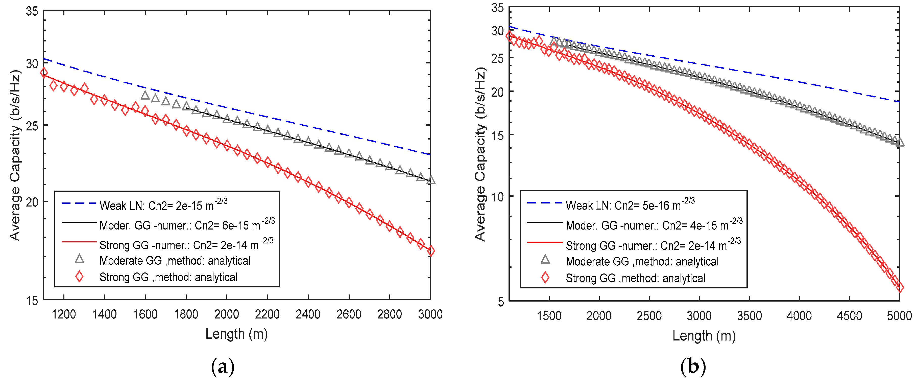
3.2. Average Channel Capacity

Another significant quantity that can be used for FSO’s performance estimation is the average capacity of the optical channel. In practice, this metric represents the practical capacity, i.e., the maximum data rate, which can be supported by the optical channel under the specific circumstances. The average capacity $\langle C\rangle$ is given as [13,36]:

$$\langle C\rangle =B{\displaystyle \underset{0}{\overset{\infty }{\int }}}{\log }_2\left(1+\frac{{\left(\eta I{P}_r\right)}^2}{N_0}\right)f_I\left(I\right)dI,$$

(18)

where B stands for the system’s bandwidth.

From the average channel capacity mathematical expression [13,28,29], and using Equation (11), we obtain the following accurate approximate expression, as a function of the transmitted power, the attenuation parameters, the fog and the scintillation effect:

$$\begin{gathered} \langle \tilde{C}\rangle =C_0\left\{{\displaystyle \sum _k}\frac{a_k}{k}\left[erfcx\left(\sqrt{2}\sigma k+\frac{A}{2\sqrt{2}\sigma }\right)+erfcx\left(\sqrt{2}\sigma k-\frac{A}{2\sqrt{2}\sigma }\right)\right]+\frac{4\sigma }{\sqrt{2\pi }}+{\rm A}exp\left(\frac{A^2}{8{\sigma }^2}\right)erfcx\left(-\frac{A}{2\sqrt{2}\sigma }\right)\right\} \\ A=ln\left(\frac{{\left(\eta P_T G_T{G}_R{\left(\frac{\lambda }{4\pi L}\right)}^2{\left(\frac{D_R}{D_T+\theta \cdot L}\right)}^2{10}^{-\left(L\cdot a_{tot}+L_m\right)/10}\right)}^2}{\left(4{{\rm K}}_{{\rm B}}{{\rm T}}_{abs}B\cdot F_n/R_L\right)+2q_{e}B\left(I_{ph}+I_D\right)+2B{\eta }^2{N}_b^2{B}_f/r+\left(RIN\right){I_{ph}}^2}\right)-{\sigma }^2, \end{gathered}$$

(19)

where $\langle \tilde{C}\rangle =\langle C\rangle /B$ and $C_0=\left(\exp \left(-A^2/8{\sigma }^2\right)\right)/\left(2\ln \left(2\right)\right)$, while the eight a_k parameters that are taken into account are given in [13,29].

Similarly to the previous case for weak turbulence conditions, for the case of moderate to strong turbulence, the average capacity is estimated through expression (18), but, in this case, with the gamma–gamma statistical distribution model. Thus, from [3,14,36], and using the expression (10), we reach a conclusion of the following closed form mathematical expression for the FSO’s average capacity, as a function of the transmitted power and the the attenuation parameters due to the fog and the scintillation effect:

$$\begin{array}{l}\langle \tilde{C}\rangle \\ =\left(\frac{{\left[{\left(ab\right)}^2\left(4{{\rm K}}_{{\rm B}}{{\rm T}}_{abs}B{F}_n/R_L+2q_{e}B\left(I_{ph}+I_D\right)+2B{\eta }^2{N}_b^2{B}_f/r+\left(RIN\right){I_{ph}}^2\right)\right]}^{\left(a+b\right)/4}}{4\mathsf{\pi }\ln \left(2\right)\Gamma \left(a\right)\Gamma \left(b\right){\left(\eta P_T G_T{G}_R{\left(\frac{\lambda }{4\pi L}\right)}^2{\left(\frac{D_R}{D_T+\theta \cdot L}\right)}^2{10}^{-\left(L{a}_{tot}+L_m\right)/10}\right)}^{\frac{a+b}{2}}}\right)\\ \times G_{2,3}^{6,1}\left(\frac{{\left(ab\right)}^2\left(\frac{4{{\rm K}}_{{\rm B}}{{\rm T}}_{abs}B{F}_n}{R_L}+2q_{e}B\left(I_{ph}+I_D\right)+\frac{2B{\eta }^2{N}_b^2{B}_f}{r}+\left(RIN\right){I_{ph}}^2\right)}{{\left(4\eta P_T G_T{G}_R{\left(\frac{\lambda }{4\pi L}\right)}^2{\left(\frac{D_R}{D_T+\theta \cdot L}\right)}^2{10}^{-\left(L{a}_{tot}+L_m\right)/10}\right)}^2}\right|\begin{array}{c}-\frac{a+b}{4},-\frac{a+b}{4}+1\\ \frac{a-b}{4},\frac{a-b+2}{4},\frac{b-a}{4},\frac{b-a+2}{4},-\frac{a+b}{4},-\frac{a+b}{4}\end{array})\end{array}$$

(20)

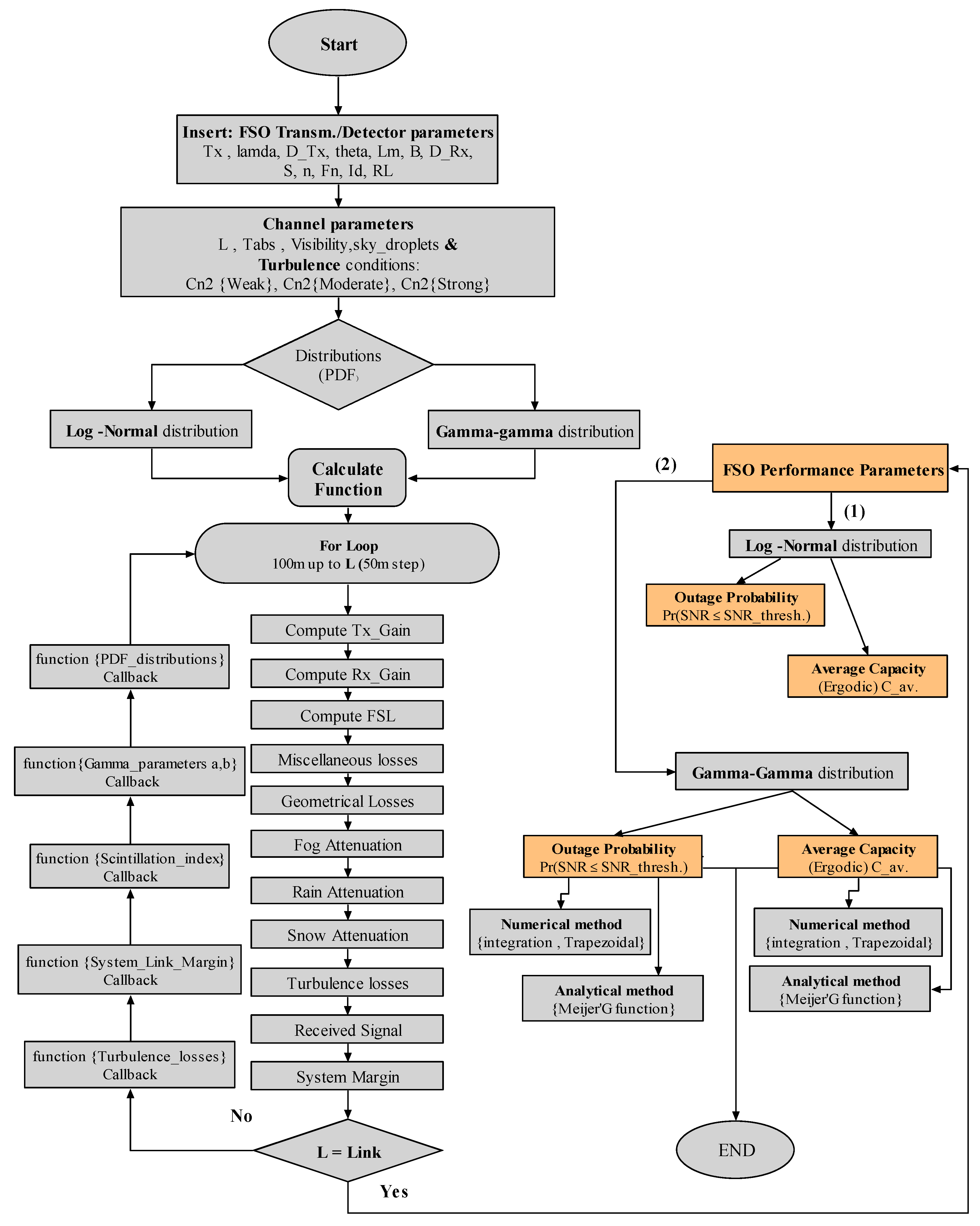
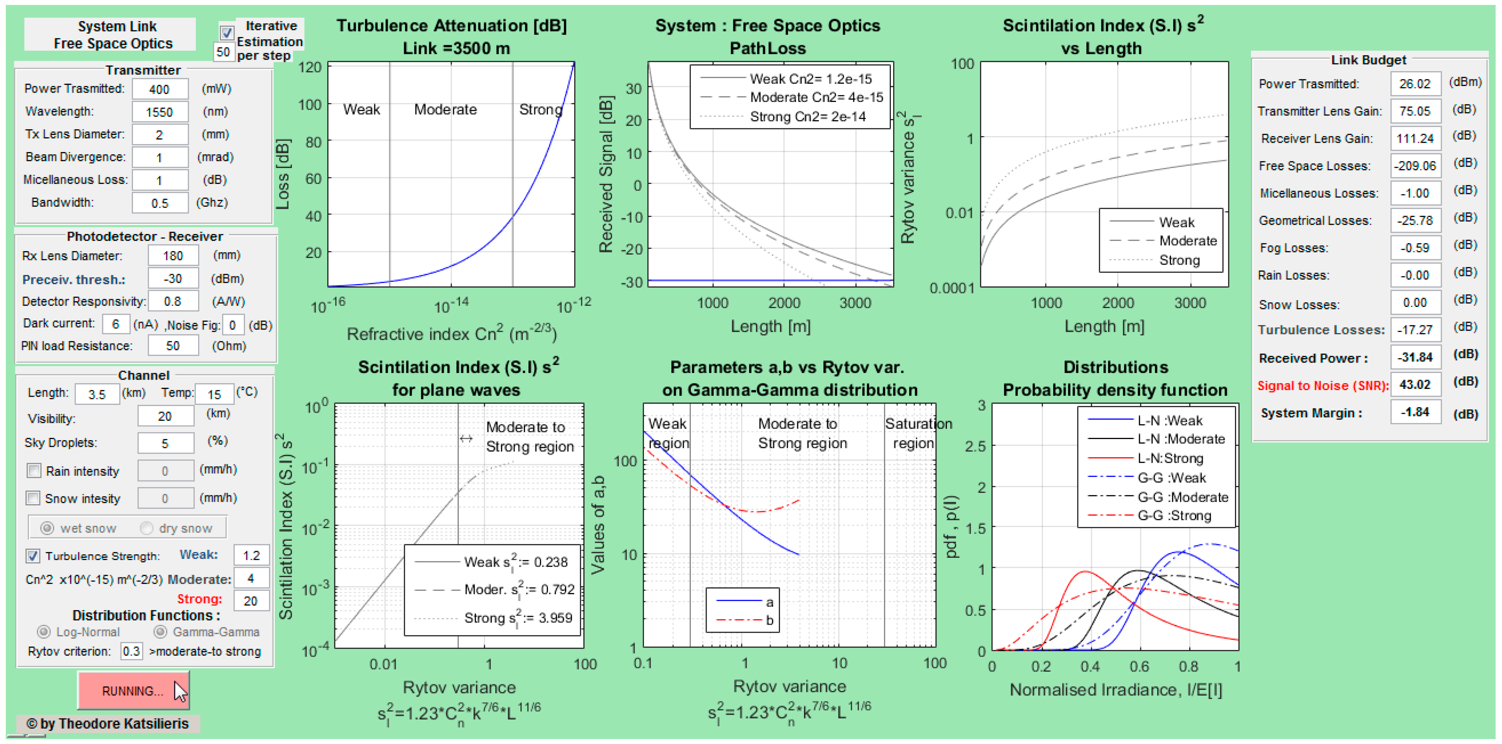
4. Algorithm Structure for the Computational Tool

Here, we present the algorithm structure of the computational tool, which is the main scope of this work and evaluates the performance of an FSO link, as a function of the link parameters, the transmitted power and the attenuation due to the fog and scintillation effect, by means of the estimation of the outage probability and average capacity metrics. Moreover, here, we assume that the ambient noise, although, in general, is a significant mitigation factor for the system’s performance, can have its influence be suppressed significantly using the suitable infrared filters. Thus, for the specific computational tool that we present below, we use the above derived Equations (16) and (17) for the outage probability estimation and Labels (19) and (20) for the average capacity, for weak or moderate to strong turbulence conditions, respectively, assuming that the ambient noise can be considered neglected [48].

The entire tool has been designed on a Graphical User Interface (GUI) that is quite easy and user-friendly. Figure 1 presents a schematic diagram of the algorithm and the numerical tool and fully describes its operation while, in Figure 2, the GUI is shown. The user must insert values for all of the initial parameters and then the calculations can be performed.

In Figure 1, it is shown that the tool has a main function, the calculate function, which controls other functions to evaluate and present the results both numerically and graphically inside the loop until achieving the case L = “Link”, i.e., “Link” representing the total link length, and estimating the SNR values for the current parameters for these conditions. Then, the code estimates the specific system performance metrics, i.e., outage probability and average capacity, for weak or moderate to strong turbulence conditions, using the lognormal or the gamma–gamma distribution, respectively. The obtained numerical results appear in new pop-up figures. To compute accurately the above-mentioned performance parameters, in the specific tool, we use both numerical and analytical methods (see Equations (16), (17), (19) and (20) and Appendix A), and obtained results are compared.

The transition point, which represents the upper limit of the weak turbulence regime, depends on the value of the Rytov parameter. More specifically, for ${\sigma }_l^2$ smaller than the critical value “0.3”, the turbulence strength is assumed to be weak and the lognormal distribution model and the corresponding mathematical expressions derived above are used. On the other hand, for ${\sigma }_l^2$ larger than “0.3”, the turbulence strength is assumed to be moderate or strong and the expressions obtained with the gamma–gamma distribution model are used. In all of the above-mentioned cases, the user of the computational tool should insert the link parameters and the attenuation strength.

5. Numerical Results

As mentioned above, the described computational tool performs calculations for the performance estimation of FSO links according to their operational parameters. Typical values for these parameters are given in Table 1. However, it is worth mentioning here that any other parameter values can be used, in order to investigate the performance of each optical wireless communication system. Taking into account the fact that this tool not only uses the theoretical mathematical expressions presented above, but also the numerical estimation methods, it is clear that the specific performance metrics can be estimated accurately for almost any practical case.

In Table 1, we present some common values that have been inserted in the proposed computational tool. These values have been used as initial conditions as can be seen in Figure 2. The way that the results are obtained is described analytically in the block diagram of the code in Figure 1. More specifically, three values of the parameter $C_n^2$ have been used, i.e., 7.8 × 10⁻¹⁶ m^−2/3, 6.0 × 10⁻¹⁵ m^−2/3, $C_n^2$ = 20.0 × 10⁻¹⁵ m^−2/3, for weak, moderate and strong turbulence conditions, respectively [36], for link lengths up to 5 km. For these parameter values and contiguous to these, by using the specific computational tool, the following figures for the presented above performance metrics are obtained.

Thus, in Figure 3a, the outage probability curves are presented for weak to strong turbulence strength and for the −30 dBm receiver’s threshold. It is clear that for weak turbulence the optical system can work reliably even for link distances up to 3.5 km. In Figure 3b, we use a −40 dBm receiver threshold for similar $C_n^2$ parameters for links up to 5 km. From the above figures, it is obvious that decreasing the receiver’s threshold increases the availability of the system. In addition, for stronger atmospheric turbulence effects, the total effective link length falls below 1700 m. However, as mentioned above, the link parameters, such as visibility, attenuation, receiver’s threshold, absolute temperature, detector responsivity, miscellaneous losses, etc., which appear in Table 1, have been used in our computational tool and produce the specific results, are changed depending on the specific optical wireless link that is investigated. Thus, if both the link and environment parameters have been studied, the proposed computational tool can be easily and accurately used for the outage performance of the link and thus for the estimation of its reliability and availability.

In Figure 4, following the same procedure as in the case with the outage probability, it is clear that the capacity performance of the channel decreases significantly when turbulence strength is getting stronger. In addition to outage probability, this performance parameter has no change from decreasing the receiver’s threshold, and thus has no dependence on this. However, it can been seen that the channel’s capacity, due to the extremely large bandwidth of the optical channel, is high enough to support high fidelity communications, even for large attenuation values, strong atmospheric turbulence effect and long link lengths. Similarly as above, the curves of Figure 4 are only results that have been obtained with the proposed computational tool and, obviously, will change if the link and atmospheric parameters are altered.

Another very significant conclusion from Figure 3 and Figure 4 is that the analytical and the numerical results for both performance quantities, i.e., outage probability and average capacity, are very close to each other. This remark confirms that the approximate or the exact mathematical Equations (16), (17), (19) and (20), which have been presented above, are accurate enough to present in an FSO link in detail. Thus, the computational tool that we present here potentially could be used as an effective and accurate tool for design and implementation of FSO links and networks.

From the computational tool and Figure 3 and Figure 4, we also obtain accurate numerical results, which are included in

Table 2. Outage probability for an FSO link with the parameters of Table 1.

Threshold	Length	${\mathit{C}}_{\mathit{n}}^{\mathbf{2}}$ (m−2/3)	Rytov Variance 1, ${\mathit{\sigma }}_{\mathit{l}}^{\mathbf{2}}$	Outage Probability		SNR, μ (dB)
				Pr (<10−3)	Drop System
		1.0 × 10−15	0.253	0.00065	3450 m	62.08
−30 dB	4 km	8.0 × 10−15	2.023	0.00046	2100 m	47.88
		2.0 × 10−14	5.057	0.00044	1700 m	33.87
		7.8 × 10−16	0.297	5.4 × 10−7		54.52
−40 dBm	5 km	6 × 10−15	2.284	0.00070	3050	38.53
		2.0 × 10−14	7.613	0.00057	2250	17.00

¹ ${\sigma }_l^2$ ≤ 0.3 denotes weak turbulence, whereas 0.3 < ${\sigma }_l^2$ < 5 denotes moderate to strong (3).

and

Table 3. Average channel capacity for an FSO link with the parameters of Table 1.

Theshold	Length	${\mathit{C}}_{\mathit{n}}^{\mathbf{2}}$ (m−2/3)	Rytov Variance 1, ${\mathit{\sigma }}_{\mathit{l}}^{\mathbf{2}}$	Average Capacity (b/s/Hz)		SNR, μ (dB)
				Capacity	Distribution
		2 × 10−15	0.298	22.91	LN	69.11
−40 dBm	3 km	6 × 10−15	0.895	21.22	GG	64.14
		2.0 × 10−14	2.984	17.32	GG	52.60
		5.0 × 10−16	0.190	18.63	LN	56.21
−30 dBm	5 km	4 × 10−15	1.523	14.18	GG	43.24
		2.0 × 10−14	7.613	5.46	GG	17.00

¹ ${\sigma }_l^2$ ≤ 0.3 denotes weak turbulence, whereas 0.3 < ${\sigma }_l^2$ < 5 denotes moderate to strong (3).

.

Table 2 and Table 3 present the performance results for an FSO link with parameters shown in Table 1. From the above results, we use the lognormal distribution that is used to simulate weak turbulence strength, i.e., Rytov variance smaller than 0.3. Under these conditions, the obtained results show maximum effective link value of about 3.45 km with availability above 99.9%, i.e., P_out ≅ 6.5 × 10⁻⁴. In addition, the normalized average capacity also has the maximum efficiency of 18.63 (b/s/Hz) for weak turbulence conditions at 5 km. For longer link lengths, the scintillation effect strongly affects the system’s operation, and, thus, the lognormal distribution cannot give accurate results. For this reason, for moderate to strong turbulence conditions, i.e., ${\sigma }_l^2$ > 0.3, we use the gamma–gamma distribution [1,3,21,30]. Thus, from Figure 3 and Figure 4 and Table 2 and Table 3, it is clear that when the turbulence strength increases, the system’s performance decreases significantly.

Due to complexity of the above derived mathematical expressions, for the case of gamma–gamma distribution (see Appendix A), the estimation of the average capacity and outage probability metric is attained from our tool with two methods. First, we evaluate the results from Equations (17) and (20) and by numerically integrating Equations (13) and (18), respectively. This procedure is followed in order to verify our results before the presentation of the final results. The worst turbulence case that we simulate was at 5 km with ${\sigma }_l^2$ = 7.613 and the system’s average capacity was 5.46 b/s/Hz with signal level SNR at 17.00 dB.

6. Conclusions

In this work, we studied an FSO link and we present approximate and exact mathematical expressions for the estimation of its performance by means of the evaluation of its average capacity and outage probability as functions of the transmitted power, the ambient noise and the attenuation parameters due to the propagation of the optical beam through the atmosphere. The obtained mathematical expressions have been derived for weak up to strong turbulence conditions, using the suitable statistical distribution models, i.e., the lognormal or the gamma, respectively, in order to describe accurately the resulting irradiance fluctuations. Based on the obtained mathematical expressions, we design and present in detail an accurate computational tool for the estimation of the performance of the FSO links, taking into account realistic values for its parameters, depending on the specific atmospheric conditions in the place where the FSO link will be installed. Moreover, this computational tool has been designed to estimate the performance results using both the theoretical expressions and the numerical evaluation. This way, the obtained performance results are estimated with two methods and the extracted computational results are verified. Thus, this computational application can be used for the performance estimation of an FSO link or even a more complex network architecture, with the necessary modifications. Finally, using the presented tool, we present numerical results for the average capacity and the outage probability of common FSO links, and we discuss their behavior for common parameter values for practical FSO links.

References

1. Ghassemlooy, Z.; Popoola, W.O. Terrestrial Free-Space Optical Communications. In Mobile and Wireless Communications: Network Layer and Circuit Level Design, 1st ed.; Fares, S.A., Adachi, F., Eds.; InTech: Rijeka, Coatia, 2010. [Google Scholar]
2. Henniger, H.; Wilfert, O. An Introduction to Free-Space Optical Communications. Radioengineering 2010, 19, 203–212. [Google Scholar]
3. Majumdar, A.K. Advanced Free Space Optics (FSO): A System Approach, 1st ed.; Springer Series in Optical Sciences: New York, NY, USA, 2015; Volume 186. [Google Scholar] [CrossRef]
4. Khalighi, M.A.; Uysal, M. Survey on Free Space Optical Communication: A Communication Theory Perspective. IEEE Commun. Surv. Tutor. 2014, 16, 2231–2258. [Google Scholar] [CrossRef]
5. Michael, S.; Parenti, R.R.; Walther, F.G.; Volpicelli, A.M.; Moores, J.D.; Wilcox, W.J.; Murphy, R. Comparison of scintillation measurements from 5 km communications link to standard statistical models. In SPIE Atmospheric Propagation VI; Thomas, L.M.W., Gilbreath, G.C., Eds.; SPIE: Orlando, FL, USA, 2009; Volume 7324, ISBN 9780819475909. [Google Scholar]
6. Libich, J.; Zvanovec, S. Measurements Statistics of three joint wireless optical links. In Proceedings of the International Workshop on Optical Wireless Communications (IWOW), Pisa, Italy, 22 October 2012.
7. Perez, J.; Zvanovec, S.; Ghassemlooy, Z.; Popoola, W.O. Experimental characterization and mitigation of turbulence induced signal fades within an ad hoc FSO network. Opt. Soc. Am. 2014, 22. [Google Scholar] [CrossRef] [PubMed]
8. Mazin, A.A.A. Performance Analysis of the Fog Effect on Free Space Optical Communication System. IOSR J. Appl. Phys. (IOSR-JAP) 2015, 7, 16–24. [Google Scholar]
9. Popoola, W.O.; Ghassemlooy, Z.; Leitgeb, E. BER and Outage Probability of DPSK Subcarrier Intensity Modulated Free Space Optics in Fully Developed Speckle. J. Commun. 2009, 4, 546–554. [Google Scholar] [CrossRef]
10. Sandalidis, H.G.; Tsiftsis, T.A.; Karagiannidis, G.K. Optical wireless communications with heterodyne detection over turbulence channels with pointing errors. J. Lightwave Technol. 2009, 27, 4440–4445. [Google Scholar] [CrossRef]
11. Gappmair, W. Novel results on pulse-position modulation performance for terrestrial free-space optical links impaired by turbulent atmosphere and pointing errors. IET Commun. 2012, 6, 1300–1305. [Google Scholar] [CrossRef]
12. Gappmair, W.; Hranilovic, S.; Leitgeb, E. Performance of PPM on Terrestrial FSO Links with Turbulence and Pointing Errors. IEEE Commun. Lett. 2010, 14, 468–470. [Google Scholar] [CrossRef]
13. Laourine, A.; Stephenne, A.; Affes, S. Estimating the Ergodic Capacity of Log Normal Channels. IEEE Commun. Lett. 2007, 11, 568–570. [Google Scholar]
14. Epple, B. Simplified channel model for simulation of free-space optical communications. IEEE/OSA J. Opt. Commun. Netw. 2010, 2, 293–304. [Google Scholar] [CrossRef]
15. Peppas, K.P.; Stassinakis, A.N.; Topalis, G.K.; Nistazakis, H.E.; Tombras, G.S. Average Capacity of Optical Wireless Communication Systems Over I-K Atmospheric Turbulence Channels. IEEE/OSA J. Opt. Commun. Netw. 2012, 4, 1026–1032. [Google Scholar] [CrossRef]
16. Andrews, L.C.; Phillips, R.L. I-K distribution as a universal propagation model of laser beams in atmospheric turbulence. J. Opt. Soc. Am. A 1985, 2, 160–163. [Google Scholar] [CrossRef]
17. Al-Habash, M.A.; Andrews, L.C.; Phillips, R.L. Mathematical model for the irradiance probability density function of a laser beam propagating through turbulent media. Opt. Eng. 2001, 40, 1554–1562. [Google Scholar] [CrossRef]
18. Kamalakis, T.; Sphicopoulos, T.; Muhammad, S.S.; Leitgeb, E. Estimation of the power scintillation probability density function in free-space optical links by use of multicanonical Monte Carlo sampling. Opt. Lett. 2006, 31, 3077–3079. [Google Scholar] [CrossRef] [PubMed]
19. Garrido, J.M.; Balsells, A.; Jurado-Navas, J.; Paris, F.; Castillo-Vasquez, M.; Puerta-Notario, A. On the capacity of M-distributed atmospheric optical channels. Opt. Lett. 2013, 38, 3984–3987. [Google Scholar] [CrossRef] [PubMed]
20. Varotsos, G.K.; Nistazakis, H.E.; Volos, C.K.; Tombras, G.S. FSO Links with Diversity Pointing Errors and Temporal Broadening of the Pulses Over Weak to Strong Atmospheric Turbulence Channels. Opt. Int. J. Light Electron Opt. 2016, 127, 3402–3409. [Google Scholar] [CrossRef]
21. Vetelino, F.S.; Young, C.; Andrews, L. Fade statistics and aperture averaging for Gaussian beam waves in moderate-to-strong turbulence. Opt. Soc. Am. Appl. Opt. 2007, 46, 3780–3789. [Google Scholar] [CrossRef]
22. Djordjevic, G.T.; Petkovic, M.I. Average BER performance of FSO SIM-QAM systems in the presence of atmospheric turbulence and pointing errors. J. Mod. Opt. 2016, 63, 715–723. [Google Scholar] [CrossRef]
23. Wilson, S.G.; Braudt-Pearce, M.; Cao, Q.; Leveque, J.H. Free-Space Optical MIMO Transmission with Q-ary PPM. IEEE Trans. Commun. 2005, 53, 1402–1412. [Google Scholar] [CrossRef]
24. Prabu, K.; Bose, S.; Kumar, D.S. BPSK based subcarrier intensity modulated free space optical system in combined strong atmospheric turbulence. Opt. Commun. 2013, 305, 185–189. [Google Scholar] [CrossRef]
25. Nistazakis, H.E.; Assimakopoulos, V.D.; Tombras, G.S. Performance estimation of free space optical links over negative exponential atmospheric turbulence channels. Opt. Int. J. Light Electron Opt. 2011, 122, 2191–2194. [Google Scholar] [CrossRef]
26. Zvanovec, S.; Perez, J.; Ghassemlooy, Z.; Rajbhandari, S.; Libich, J. Route diversity analyses for free-space optical wireless links within turbulent scenarios. Opt. Express 2013, 21, 7641–7650. [Google Scholar] [CrossRef] [PubMed]
27. Nistazakis, H.E.; Katsis, A.; Tombras, G.S. On the reliability and performance of fso and hybrid fso communication systems over turbulent channels. In Turbulence: Theory, Types and Simulations; Nova Science Publishers: Hauppauge, NY, USA, 2011. [Google Scholar]
28. Laourine, A.; Stephenne, A.; Affes, S. Capacity of Log Normal Fading Channels. In Proceedings of the International Conference on Wireless Communications and Mobile Computing 2007 (IWCMC2007), Honolulu, HI, USA, 12–17 August 2007; pp. 13–17.
29. Nistazakis, H.E.; Tsiftis, T.A.; Tombras, G.S. Performance analysis of the free space optical communications systems over atmospheric turbulence channel. IET Commun. 2009, 3, 1402–1409. [Google Scholar] [CrossRef]
30. Vetelino, F.S.; Young, C.; Andrews, L.; Recolons, J. Aperture averaging effects on the probability density of irradiance fluctuations in moderate to strong turbulence. Opt. Soc. Am. Appl. Opt. 2007, 46. [Google Scholar] [CrossRef]
31. Bekkali, A.; Naila, C.B.; Kazaura, K.; Wakamori, K.; Matsumoto, M. Transmission Analysis of OFDM-Based Wireless Services Over Turbulent Radio-on-FSO links Modeled by Gamma-Gamma Distribution. IEEE Photonics J. 2010, 2, 510–520. [Google Scholar] [CrossRef]
32. Stassinakis, A.N.; Nistazakis, H.E.; Tombras, G.S. Comparative Performance Study of One or Multiple Receivers Schemes for FSO Links Over Gamma Gamma Turbulence Channels. J. Mod. Opt. 2012, 59, 1023–1031. [Google Scholar] [CrossRef]
33. Katsilieris, T.D.; Latsas, G.P.; Nistazakis, H.E.; Tombras, G.S. A computational tool which has been designed for performance estimations of wireless hybrid FSO/MMW communication links. In Proceedings of the 7th International Conference from Scientific Computing to Computational Engineering (IC-SCCE), Athens, Greece, 6–9 July 2016.
34. Higgs, C.; Barclay, H.T.; Murphy, D.V.; Primmerman, C.A. Atmospheric Compensation and Tracking Using Active Illumination. Linc. Lab. J. 1998, 11, 5–26. [Google Scholar]
35. Uysal, M.; Li, J.T.; Yu, M. Error rate performance analysis of coded free-space optical links over gamma–gamma atmospheric turbulence channels. IEEE Trans. Commun. 2006, 5, 1229–1233. [Google Scholar] [CrossRef]
36. Nistazakis, H.E.; Tombras, G.S.; Tsigopoulos, A.D.; Karagianni, E.A.; Fafalios, M.E. Capacity estimation of optical wireless communication systems over moderate to strong turbulence channels. J. Commun. Netw. 2009, 11, 387–392. [Google Scholar] [CrossRef]
37. Kiasaleh, K. Channel estimation for FSO channels subject to gamma–gamma turbulence. In Proceedings of the International Conference on Space Optical Systems and Applications (ICSOS2012), Corsica, France, 9–12 October 2012.
38. Kharraz, O.; Forsyth, D. PIN and APD photodetector efficiencies in the longer wavelength range 1300–1550 nm. Opt. Int. J. Light Electron Opt. 2013, 124, 2574–2576. [Google Scholar] [CrossRef]
39. Nistazakis, H.E.; Stassinakis, A.N.; Muhammad, S.S.; Tombras, G.S. BER Estimation for Multi Hop RoFSO QAM or PSK OFDM Communication Systems Over Gamma Gamma or Exponentially Modeled Turbulence Channels. Opt. Laser Technol. 2014, 64, 106–112. [Google Scholar] [CrossRef]
40. Avago Technologies. Note 922. Available online: https://docs.broadcom.com/docs/5965-8666E (accessed on 13 November 2016).
41. Gagliardi, R.M.; Karp, S. Optical Communications, 2nd ed.; John Wiley & Sons: Hoboken, NJ, USA, 1995. [Google Scholar]
42. Khalighi, M.A.; Xu, F.; Jaafar, Y.; Bourennane, S. Double-laser differential signaling for reducing the effect of background radiation in free-space optical systems. IEEE/OSA J. Opt. Commun. Netw. 2011, 3, 145–154. [Google Scholar] [CrossRef]
43. Rollins, D.; Baars, J.; Bajorins, D.; Cornish, C.; Fischer, K.; Wiltsey, T. Background light environment for free-space optical terrestrial communications links. In Proceedings of SPIE, Optical Wireless Communications V; Korevaar, E.J., Ed.; SPIE: Redmond, DC, USA, 2002; Volume 4873, pp. 99–110. [Google Scholar]
44. Mendoza, B.R.; Rodríguez, S.; Pérez-Jiménez, R.; Ayala, A.; González, O. Comparison of Three Non-Imaging Angle-Diversity Receivers as Input Sensors of Nodes for Indoor Infrared Wireless Sensor Networks: Theory and Simulation. Sensors 2016, 16, 1086. [Google Scholar] [CrossRef] [PubMed]
45. Leeb, W.R. Degradation of signal to noise ratio in optical free space data links due to background illumination. Appl. Opt. 1989, 28, 3443–3449. [Google Scholar] [CrossRef] [PubMed]
46. ITU-R Recommendation P.1814-1. Prediction Methods Required for the Design of Terrestrial Free-Space Optical Links; International Telecommunication Union: Geneva, Switzerland, 2007. [Google Scholar]
47. Muhammad, S.S.; Köhldorfer, P.; Leitgeb, E. Channel Modeling for Terrestrial Free Optical Links. In Proceedings of the 7th International Conference on Transparent Optical Networks (ICTON), Barcelona, Spain, 3–7 July 2005; pp. 407–410.
48. Tsiftsis, T.A.; Sandalidis, H.G.; Karagiannidis, G.K.; Uysal, M. FSO Links with Spatial Diversity Over Strong Atmospheric Turbulence Channels. In Proceedings of the IEEE International Conference on Communications (ICC), Beijing, China, 19–23 May 2008.
49. Adamchik, V.S.; Marichev, O.I. The Algorithm for Calculating Integrals of Hypergeometric Type Function and its Realization in Reduce System. In Proceedings of the International Conference on Symbolic and Algebraic Computation, Tokyo, Japan, 20–24 August 1990; pp. 212–224.
Figure 1. Block diagram of the computational tool.
Computation 05 00018 g001
Figure 2. The computation tool interface.
Computation 05 00018 g002
Figure 3. Outage probability estimation, with the proposed computational tool for weak to strong turbulence conditions, (a) for links up to 4 km with receiver threshold set as −30 dBm; (b) for total link length up to 5 km with receiver threshold set as −40 dBm. These results use the lognormal or the gamma–gamma distribution as mentioned in the plot legend.
Computation 05 00018 g003
Figure 4. Average capacity performance metric for weak to strong atmospheric turbulence conditions (a) for links up to 3 km with receiver threshold set as −40 dBm; (b) for links up to 5 km with receiver threshold set as −30 dBm. These results use the suitable distribution model, i.e., lognormal or gamma–gamma depending on the value of the Rytov parameter, as presented in Equation (3).
Computation 05 00018 g004