
Implicit Large Eddy Simulation of Flow in a Micro-Orifice with the Cumulant Lattice Boltzmann Method


Institute for Computational Modeling in Civil Engineering, TU Braunschweig, 38106 Braunschweig, Germany
*
Author to whom correspondence should be addressed.
Computation 2017, 5(2), 23; https://doi.org/10.3390/computation5020023
Submission received: 29 March 2017
/
Revised: 24 April 2017
/
Accepted: 27 April 2017
/
Published: 5 May 2017
(This article belongs to the Special Issue CFD: Recent Advances in Lattice Boltzmann Methods)
Abstract
:A detailed numerical study of turbulent flow through a micro-orifice is presented in this work. The flow becomes turbulent due to the orifice at the considered Reynolds numbers (∼). The obtained flow rates are in good agreement with the experimental measurements. The discharge coefficient and the pressure loss are presented for two input pressures. The laminar stress and the generated turbulent stresses are investigated in detail, and the location of the vena contracta is quantitatively reproduced.
1. Introduction
Flow through orifices is observed in many industrial applications. One example is the orifice meter used for measuring flow rates via the pressure drop induced by the constriction of the flow [1,2,3,4]. The main characteristic of flow through an orifice is that the flow velocity increases by substantially decreasing the cross-sectional flow area. Turbulent shear stresses are created downstream of the orifice. A “vena contracta” is formed inside the orifice. Turbulent eddies and recirculation of flow occur both upstream and downstream of the orifice. Theory and applications of orifice meters for measurement purposes can be found in [5,6,7,8,9].
Orifices can be used for increasing the shear stress in the flow (e.g., in order to break up suspended particles). The geometry studied in this paper was designed for this purpose, but the methodology used here applies in the same way for any kind of turbulent flow through an orifice at subsonic speeds [10,11].
Few studies have been conducted to simulate an orifice with the help of computational fluid dynamics (CFD) [12,13,14,15,16,17], and are usually focused on experimental investigations. However, measurements are not possible under all conditions (e.g., due to high pressure), and some quantities like local shear stress distributions are difficult to obtain experimentally. Most of the above-cited CFD studies considered laminar flow in the orifice or they used explicit turbulence modeling in order to capture turbulent eddies. These simplifications may reduce the overall accuracy of the CFD approach [13,18,19]. The advancement in CFD theory and in high performance computing motivates us to study orifice flow with a high-fidelity CFD method that resolves the relevant flow features in space and time. Here we use the cumulant lattice Boltzmann method (LBM) that allows the simulation of time-resolved turbulent flows at acceptable cost [20,21,22,23].
2. Aim of This Work
The aim of this work is to simulate turbulent flow in a micro-orifice [24] while resolving all essential flow features. The micro-orifice has a width of 80 μm, a height of 50 μm, and a length of 300 μm (Figure 1). It is located in the center of a channel of two centimeters in length. Only half of the geometry is displayed, since the shape is symmetric in the x-direction (however, the simulation included the full geometry). There is an asymmetry in the z-direction. Pressure, velocity, and stress distributions are studied for this special orifice. The laminar and turbulent stresses in the orifice are calculated and presented in detail.
Three input pressures corresponding to pressure drops of 100 bar, 200 bar, and 500 bar, respectively, between the entrance and the exit of the device are considered in this study. All pressures and stresses in this paper are given in bar, with 1 bar = Pa. All pressures are measured with reference to the pressure at the outlet, where we assume the pressure to be zero. In the real device, a sufficiently high pressure was applied at the outlet to suppress cavitation inside the device. This absolute pressure at the outlet can be determined a posteriori from the simulation results, and is hence no input parameter to the simulation itself. The flow setup was chosen to accurately simulate the pressure drop of 200 bar by adjusting the resolution to the boundary layer thickness.
In CFD simulations, more resolution is required when higher pressure drops are imposed, leading to larger mass fluxes and thinner boundary layers. The simulation for a pressure drop of 500 bar is already slightly under-resolved. Therefore, the results for this case have to be used with some caution, as they are expected to be less accurate than the results for the pressure drop of 200 bar.
3. The Cumulant Lattice Boltzmann Method
This study applies the cumulant lattice Boltzmann method [20]. Turbulent flow can be simulated accurately with the use of this method, as long as the computational domain is resolved adequately. The classical lattice Boltzmann equation without an external force can be written as follows:
where and are the discrete momentum distribution function and the collision operator, respectively. Here x, y, and z are positions of the lattice nodes. The lattice speed is defined as the ratio of the lattice spacing to the time step such that the distributions are shifted by from one lattice node to another on a Cartesian grid during one time step.
In order to obtain the lattice Boltzmann equation in the cumulant space, we have to transform the distribution functions into cumulants [20,25]. The lattice Boltzmann equation in cumulant space is:
where is the cumulant for the equilibrium state and , , and are three discrete random variables corresponding to the normalized microscopic velocities in x, y, and z directions.
4. Simulation Results
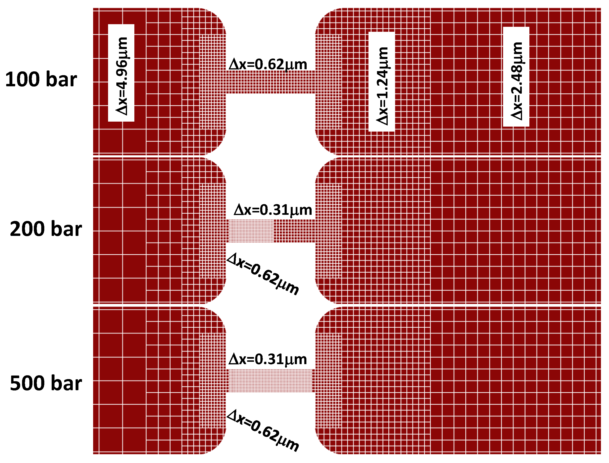
The simulation domain was discretized with nested Cartesian grids [26,27] using a block-structured code based on Esoteric Twist [28] with resolution varying from 4.96 μm to 0.62 μm for the 100 bar case and down to 0.31 μm in the 200 bar and 500 bar cases. The grid for the 100 bar case contained approximately 57 million grid nodes, the one for the 200 bar case had 65 million grid nodes, and the grid for the 500 bar case had 79 million grid nodes. The setup is shown in Figure 2, and further details are given in [21]. Turbulence emerges naturally in the cumulant lattice Boltzmann method. No fluctuations were added to the flow field. In general, high velocity gradients are observed close to the wall, which is why the highest grid resolution has to be spent there. A commonly-used grid independence criterion for CFD simulations is that the value is on the order of one or smaller [29]. For that reason, one additional grid level was spent for the pressure drops of 200 bar and 500 bar in comparison to the 100 bar case in order to keep the value close to one. The simulation required about 15 days on 120 Intel Nehalem compute nodes (2.6 GHz) with eight cores each to simulate 655 μs real time for the 200 bar case. Due to the different numbers of lattice nodes, the 100 bar case required about half the compute time of the 200 bar case, and the 500 bar case required about 1.5 times the time of the 200 bar case to reach the same real time.
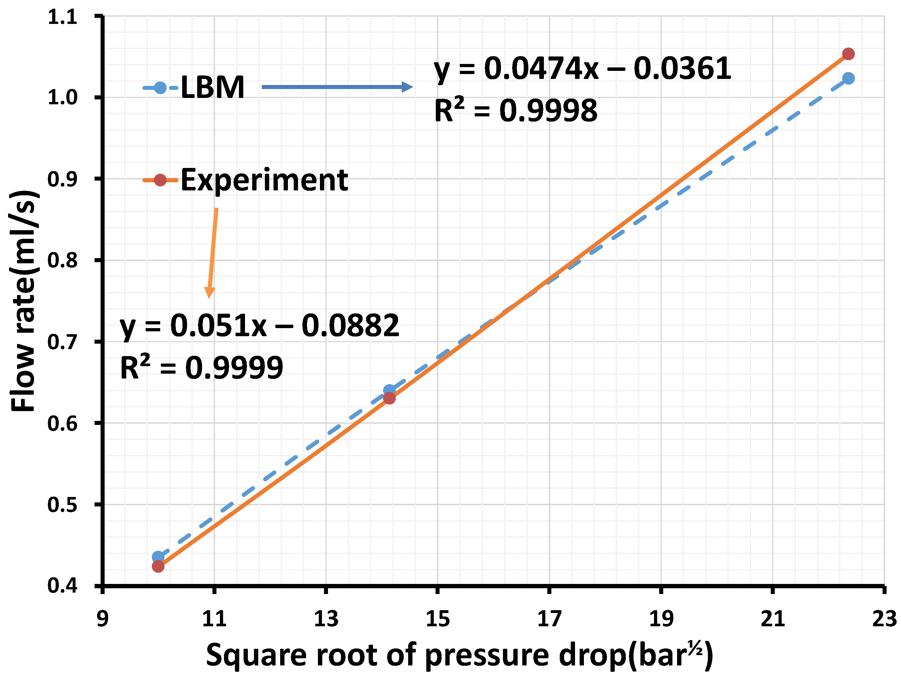
The flow rates acquired by our simulations are compared with the experimental measurement to validate our results [11]. The deviations between the LBM simulation and the experiment for the 100 bar, 200 bar, and 500 bar pressure drops are 1.57%, 1.51%, and 2.84%, respectively. It is observed that our results are in close agreement with the experimental results (see Figure 3).
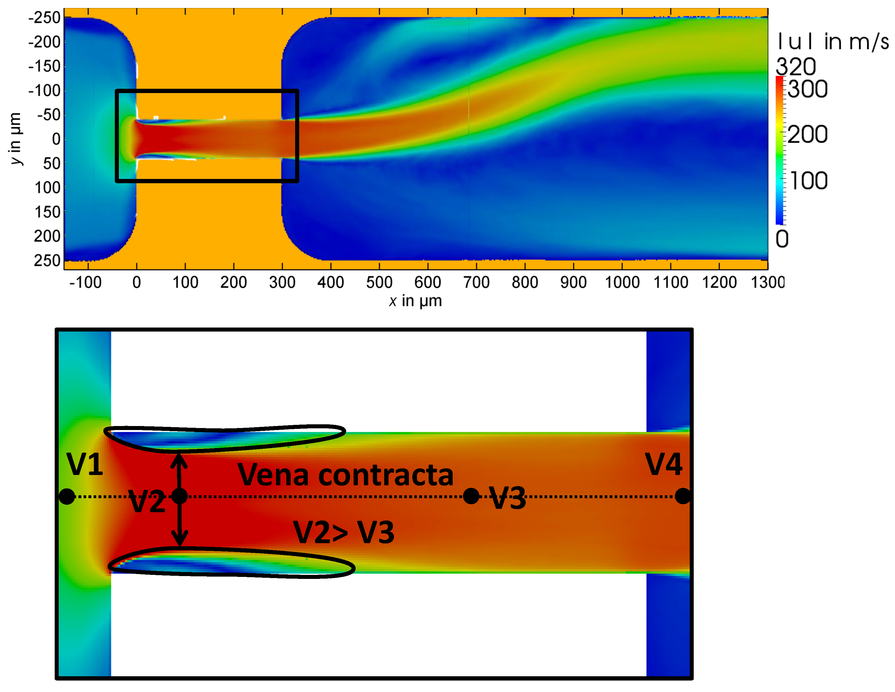
In addition to the averaged velocity, Figure 4 demonstrates the vena contracta effect. The vena contracta reduces the effective area and increases the velocity. Thus, it is observed that the velocity in position 2, , is greater than the velocity in position 3, . This phenomenon is a classical problem in fluid mechanics, and researchers try to eliminate it in some ways, such as by rounding the entrance region [30]. An orifice usually has two loss coefficients: the loss coefficient due to a sudden contraction, and the loss coefficient due to a sudden expansion. Streeter [31] calculated the loss coefficient for both a sudden contraction and a sudden expansion, and provided approximations for these coefficients in relation to the ratios of the cross-sections. For example, for a cylindrical orifice, the loss coefficients extracted from his plot are 0.42 and 0.68 for the sudden expansion and the sudden contraction, respectively. In general, these loss coefficients are related to the pressure loss calculated from the energy equation between points 1 and 2 and points 3 and 4 [30].
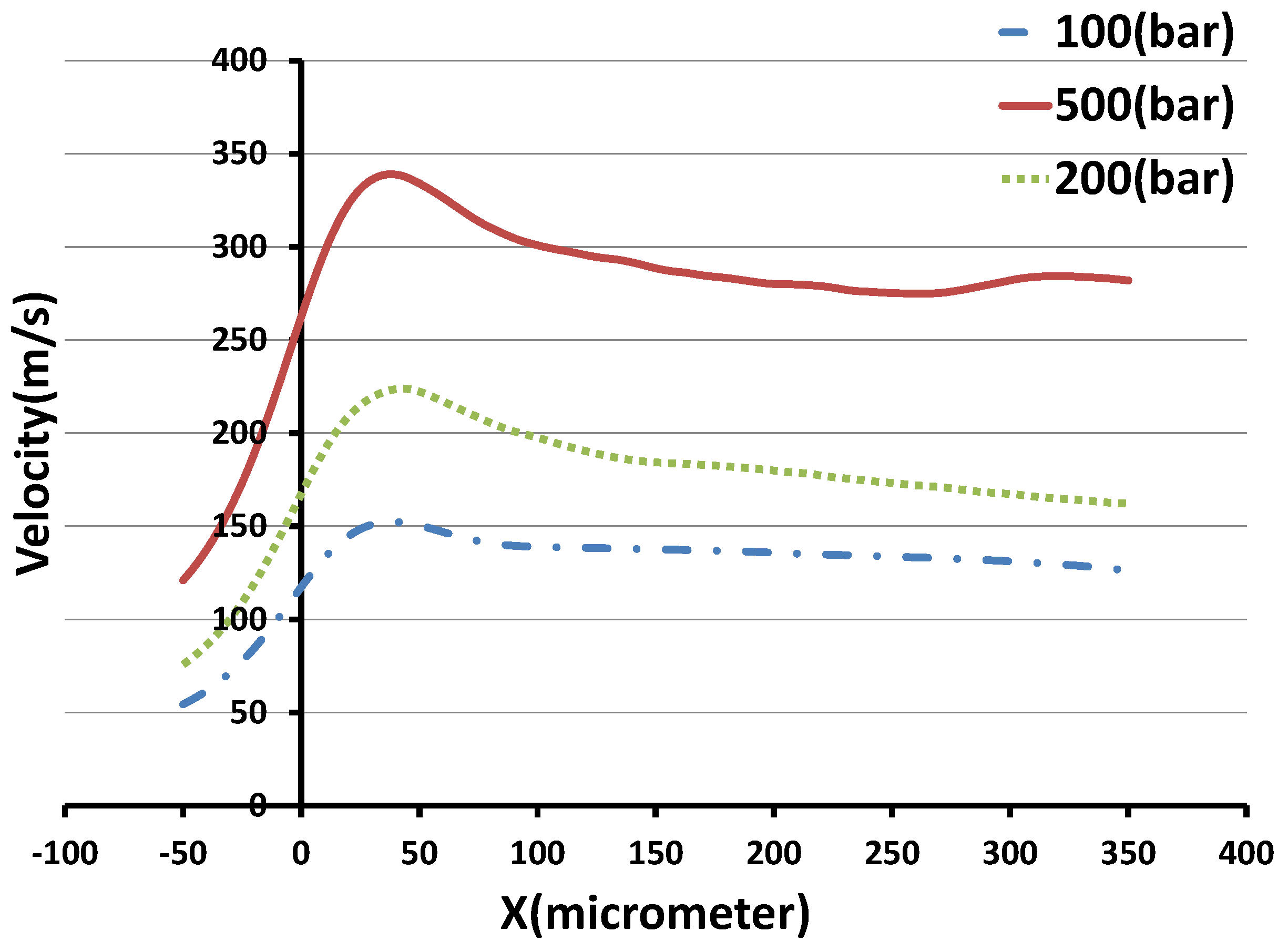
The center line magnitude velocities for three different pressure drops of 100 bar, 200 bar, and 500 bar are shown in Figure 5. The plot area covers a distance from 50 μm before the orifice entrance to 50 μm after the orifice exit. The position coincides with the entrance of the orifice. The velocity in each case reaches the maximum value at point (Figure 4).
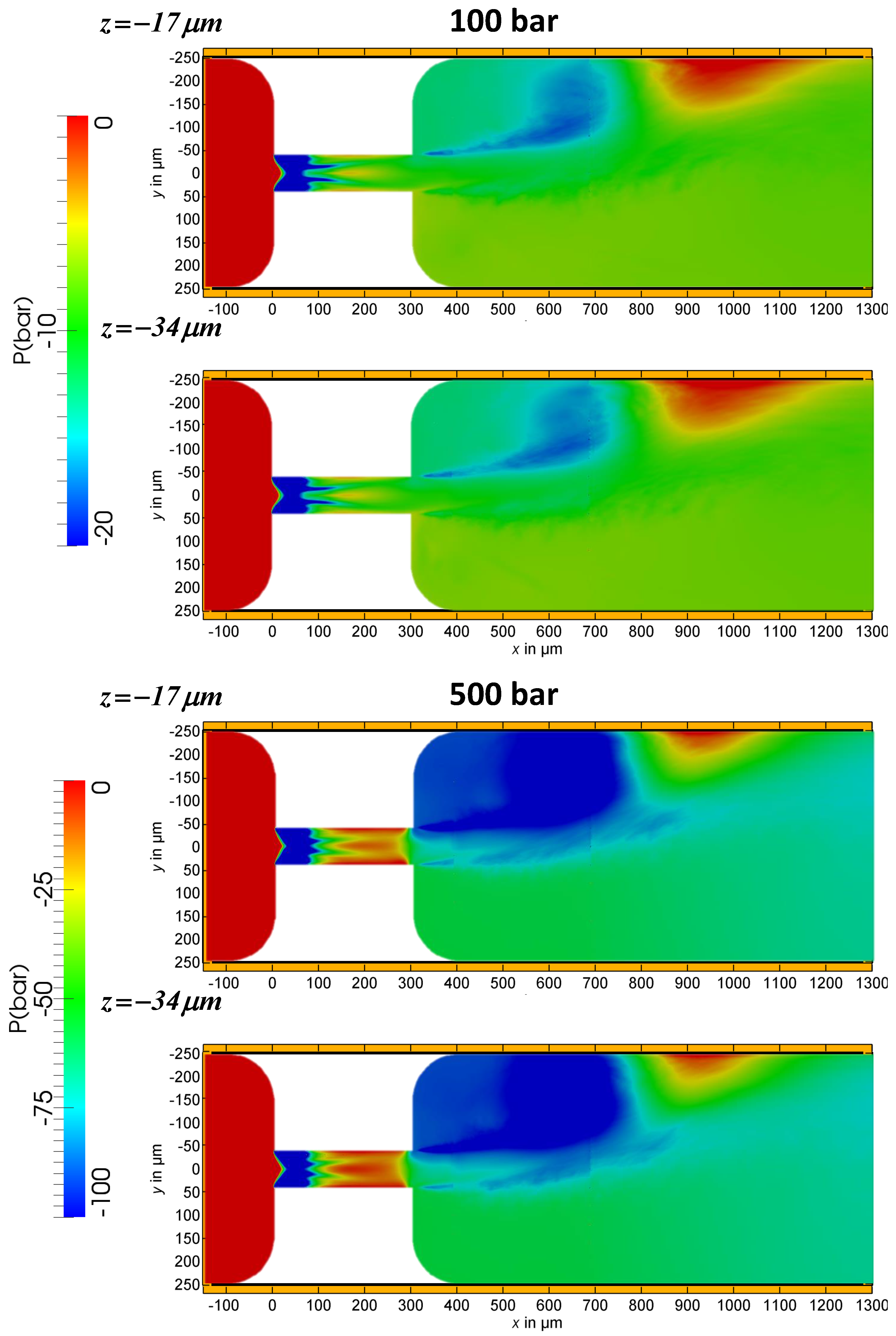
The time-averaged pressure in and behind the orifice is depicted for the 100 bar and 500 bar cases in Figure 6. It is shown for two different planes: μm and μm, according to Figure 1.
The pressure is seen to have negative values in comparison to the pressure at the outlet of the device (assumed to be zero). The device is susceptible to cavitation, which is undesired since it leads to the erosion and eventually to the destruction of the device. Cavitation is suppressed in the operation of the device by applying a sufficiently high absolute pressure at the outlet such that the minimal absolute pressure inside the device does not drop below the vapor pressure of water. Part of the purpose of the simulation was to determine the minimum pressure required at the outlet to suppress the cavitation. Since this can be done a posteriori, it was not required to consider the cavitation in the simulation itself. We note here that cavitation can be simulated with the lattice Boltzmann method, if required [32].
Figure 6 shows the reason why the jet is attached to the wall after leaving the orifice. In the volume confined by the jet and the wall in negative y direction, the pressure decreases due to the suction effect of the moving jet. This lowers the pressure in the confined volume relative to the pressure in the open volume on the other side of the jet. The pressure difference between the confined and the open volume drives the jet towards the confined volume. While the jet oscillates downstream of the orifice, it was never observed in the simulation or the experiment that the jet would switch to the other wall once it was attached.
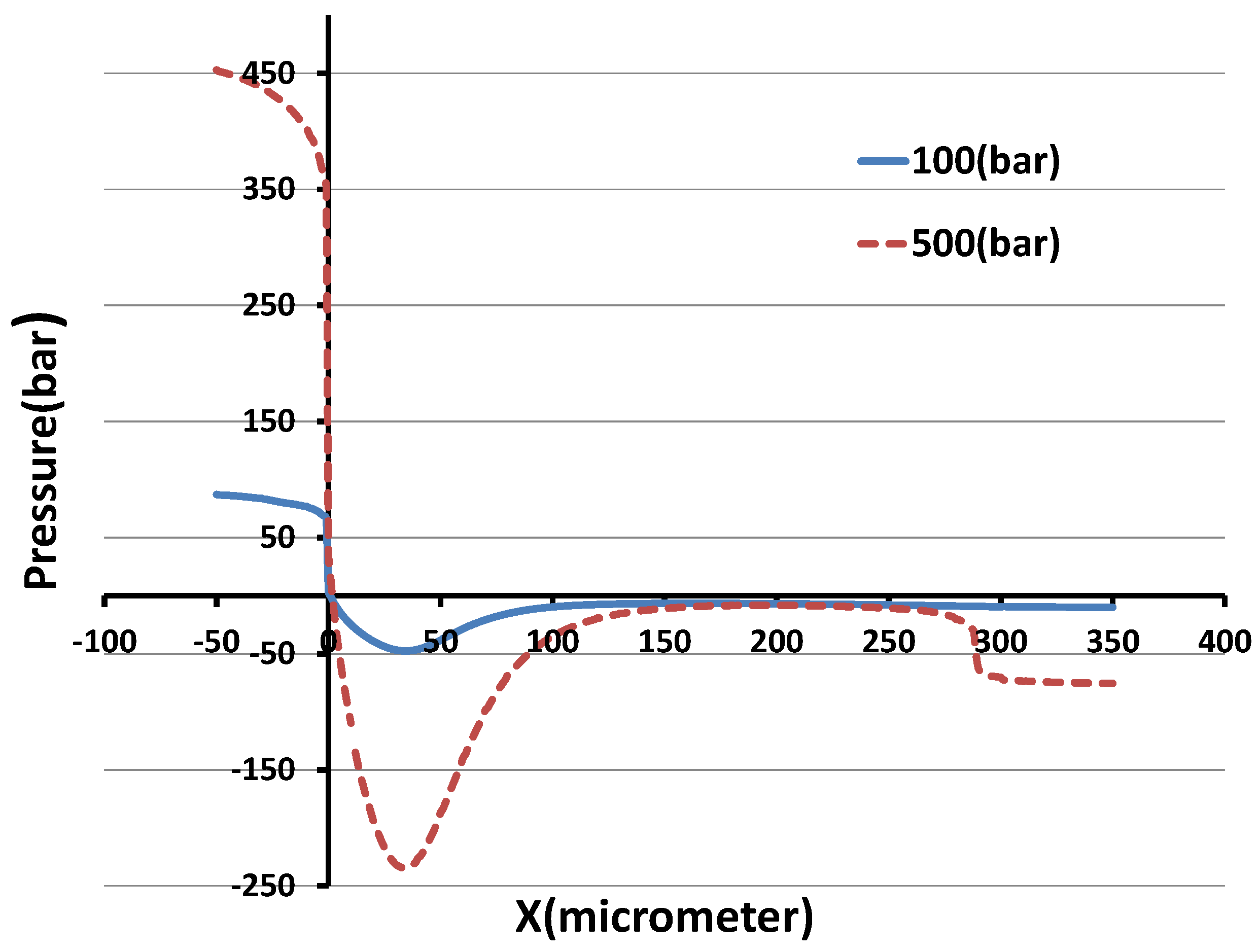
The time-averaged pressure is averaged again over the planes and plotted along the main flow direction (x direction) for the 100 bar and 500 bar cases in Figure 7. The orifice entrance is located at . The pressure drops suddenly at the entrance, and reaches its minimum value where the velocity has its maximum. The pressure drops further at the exit of the orifice. This effect is much more pronounced in the 500 bar case than in the 100 bar case. The plot displayed in Figure 7 is used to calculate the pressure loss between two points along the x direction [30]. With the flow rate known, the only required parameter for the energy equation is the pressure drop between the two points, and the discharge coefficient can be calculated (defined as the ratio of the actual flow to the theoretical flow—mean velocity × cross-section × density). The following equation has been used to calculate [33]:
where V is the averaged velocity in the orifice and is the pressure difference between upstream of the orifice and the vena contracta—at which the wall pressure is at its minimum. The ratio of the orifice diameter to the channel diameter is termed . In our case, it is determined as . The discharge coefficients for pressure drops 100 bar and 500 bar are and , respectively. The actual location of the vena contracta changes with the flow rate, and this location can be obtained from Figure 5 or Figure 7.
Tables in hydraulic handbooks list the loss coefficient only for a limited number of specific geometries. In other cases, CFD simulations as presented in this work can be used to obtain this coefficient. The averaged pressure and velocity can be extracted from Figure 3 and Figure 7, respectively. The pressure loss can be easily calculated by inserting the obtained pressures and velocities into the energy equation.
The pressure loss per length l can be calculated by the use of the following equation [34]:
where the mean velocity V is calculated from the numerically-determined mass flow, is the density of water, and is the friction factor. Since the studied orifice has a rectangular shape, the hydraulic diameter must be considered, . The Reynolds number at the smallest cross-sectional areas of the orifice is defined as:
here is the dynamic viscosity. When the device simulated here was designed, no simulations were available and the geometry was chosen based on simple considerations using the Blasius equation for round channels [10], even though the orifice is neither round nor a channel in the sense used by Blasis [35]. The roughness of the orifice is below 20 nm [10,11]; thus, the friction factor of hydraulically smooth channels at the respective Reynolds numbers () was chosen [35]:
The calculated pressure losses per millimeter in the orifice segments with the smallest cross-sectional area are 33.00 bar/mm and 150.12 bar/mm for the two pressure drops 100 bar and 500 bar, respectively.
4.1. Fluid Flow Intensity
The stresses are calculated by the velocity-gradient components. The strain rate tensor is composed of the nine velocity-gradient components, of which three are normal strain components and six are tangential strains components. The magnitude of the strain rate tensor can be written in terms of velocity gradients, as:
In order to obtain the velocity-gradients in this equation, a finite difference scheme is implemented in common CFD methods. Thus, each grid node needs information from its neighbors. In the LBM, the strain rate can be computed locally from the non-equilibrium part of the distribution function. The above equation is rewritten according to the strain rate instead of the velocity gradients as:
By convention, the magnitude of the strain rate tensor is defined as [36,37]:
where the strain rate component is:
The dissipation rate is a useful parameter for the characterization of the local hydrodynamic conditions and flow field intensities.
The total dissipation can be split up into the averaged energy dissipation rate and the turbulent dissipation rate according to the following equation [38]:
This is often done in the CFD literature due to the prevalence of Reynolds-averaged Navier–Stokes (RANS) methods. In such methods, only the average energy dissipation rate is directly accessible, and the turbulent dissipation rate must be estimated with some turbulence model. Our method provides the full information on the dissipation rate.
The corresponding stress can be acquired from:
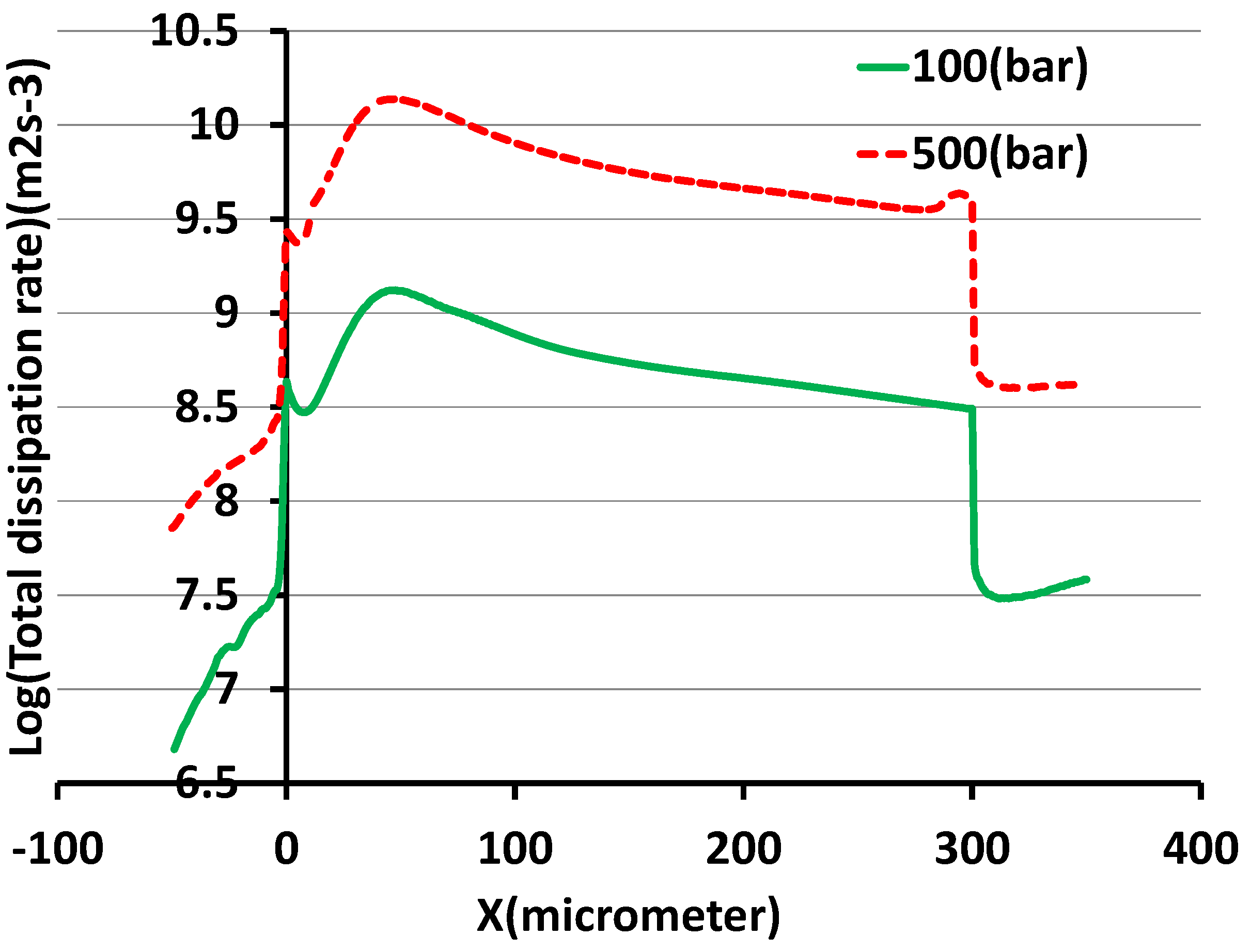
Figure 8 shows the logarithm of the dissipation rates for the 100 bar and 500 bar cases from 50 μm before to 50 μm after the orifice. There is a substantial increase in the dissipation rate at the entrance of the orifice in comparison to 50 μm in front of the entrance. Two peaks are observed in the dissipation; one is exactly at the entrance, and another one is at position μm. It is the same position where the maximal velocity and the minimal pressure are observed.
4.1.1. Q-Criterion
Both Eulerian and Lagrangian methods are available to detect coherent structures (eddies) in a flow [39,40]. Many of the Eulerian methods are based on the velocity gradient tensor [40,41,42]. One prominent example of such indicators is the Q-criterion [43], which is determined from the second invariant of the velocity gradient tensor, and is given by:
where the antisymmetric part or the vorticity tensor is:
The Q-criterion is applied to detect the dominance of the vorticity over the strain. Vorticity is dominant when , while strain is dominant for . A zero contour of Q can be used to visualize vortices.
Figure 9, Figure 10 and Figure 11 show contours for for the three cases. Q is calculated for the averaged velocity fields in these figures. Stretched vortex tubes are observed at the entrance of the orifice. With increasing pressure drop and Reynolds number, finer vortex structures develop in the orifice.
4.1.2. Laminar and Turbulent Stresses
As with dissipation, the stresses generated by the fluid flow can be divided into laminar stresses and turbulent stresses [44,45,46,47].
where and are the laminar stress tensor and turbulent stress tensor, respectively. The stress tensor is given by:
The laminar stress tensor consists of the average velocity derivatives [44]:
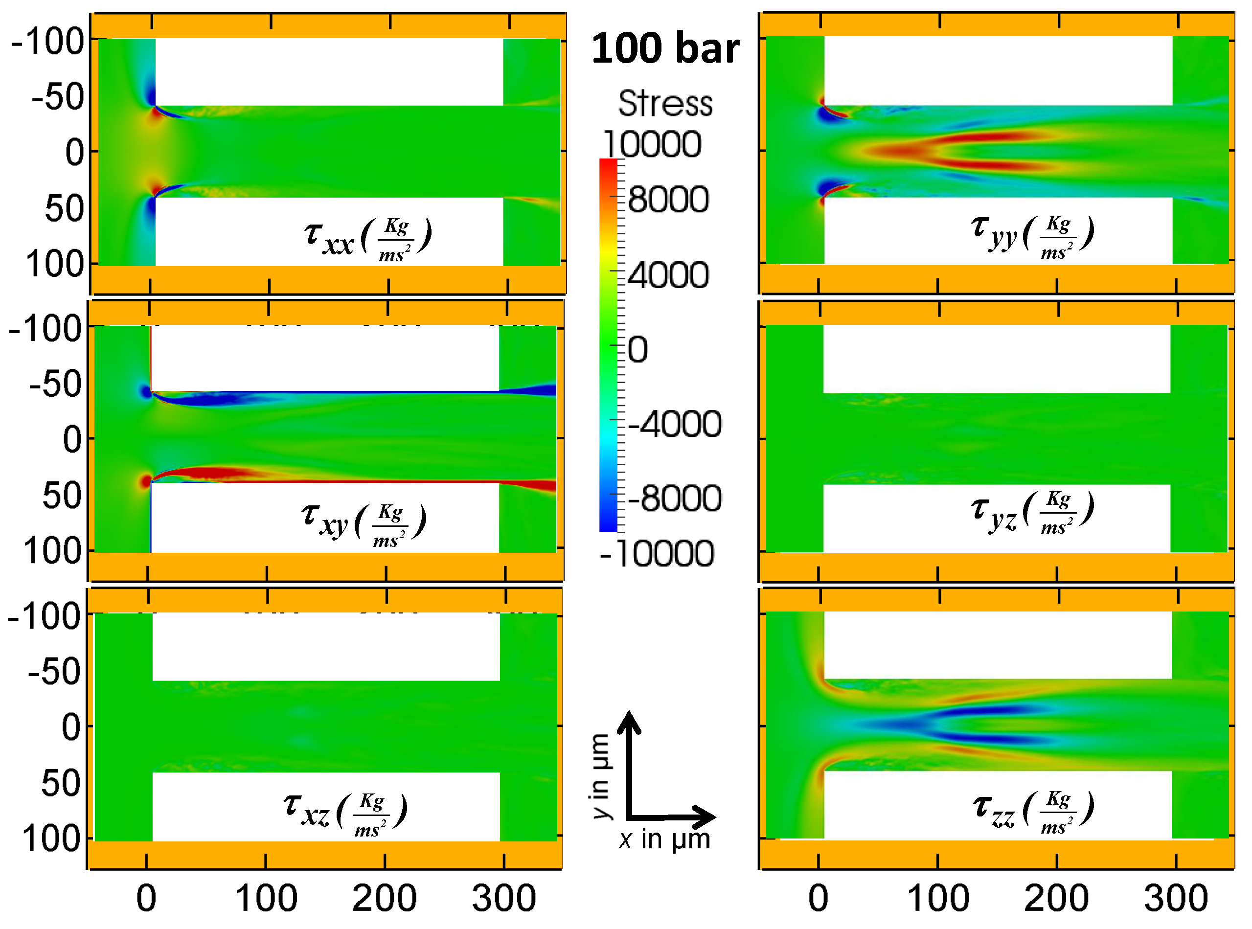
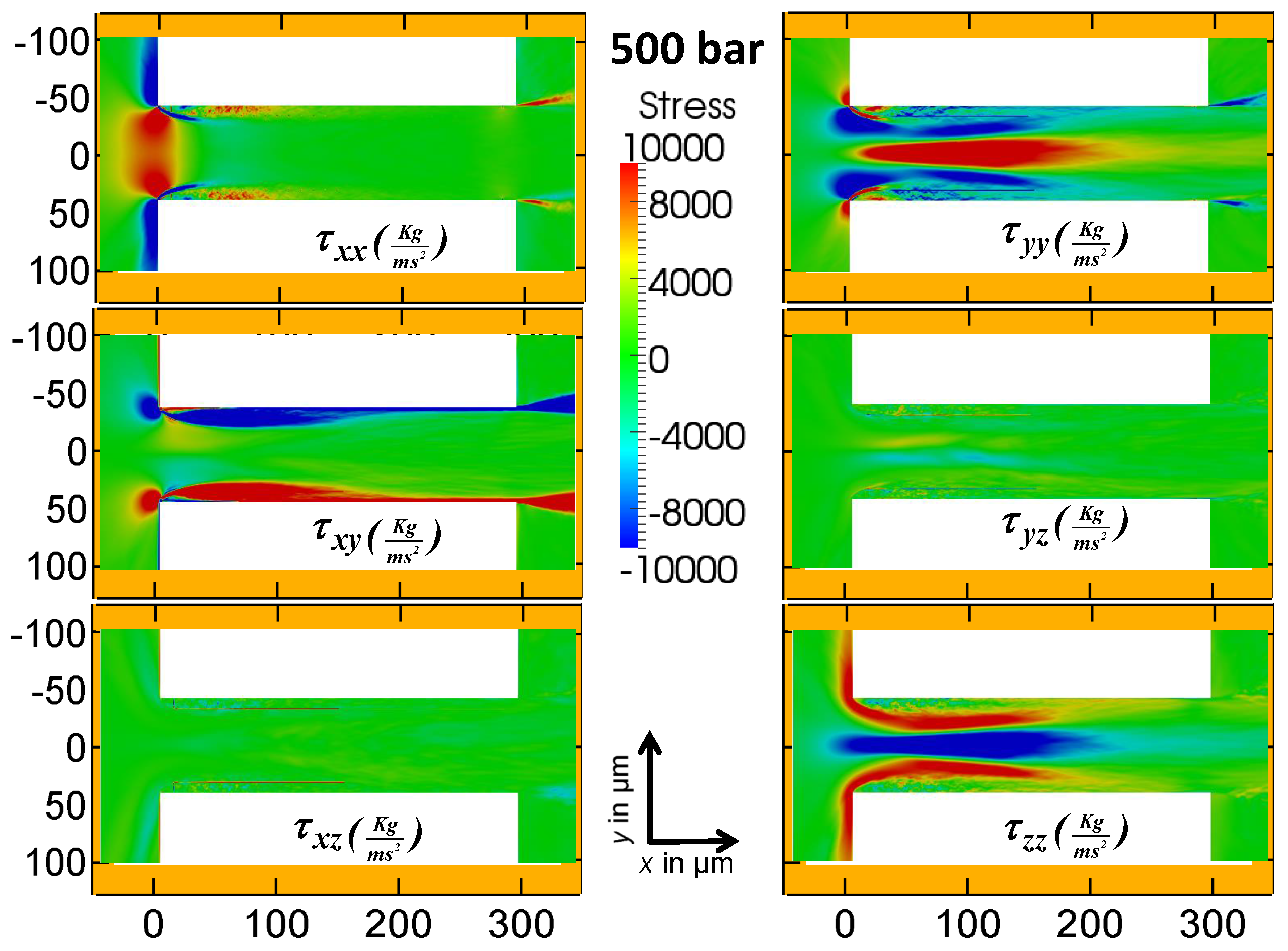
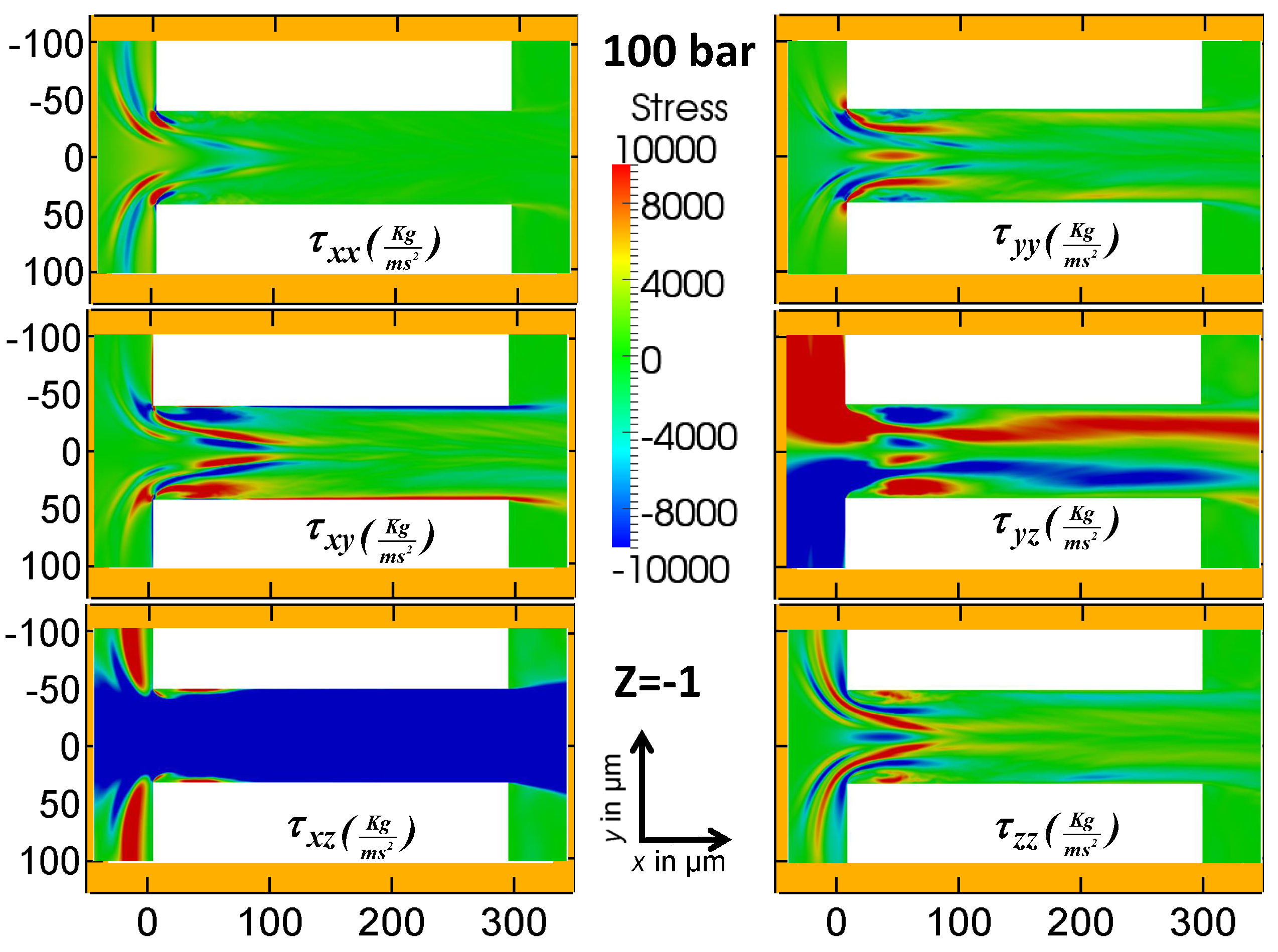
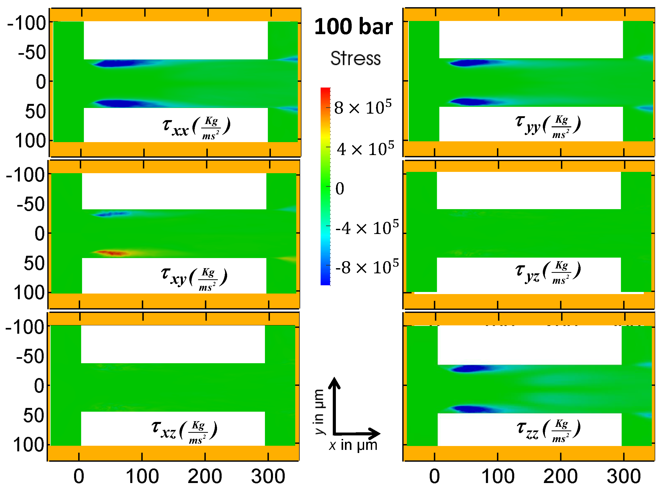
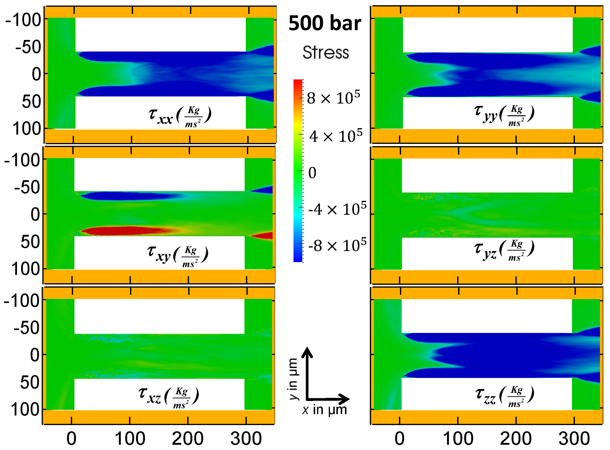
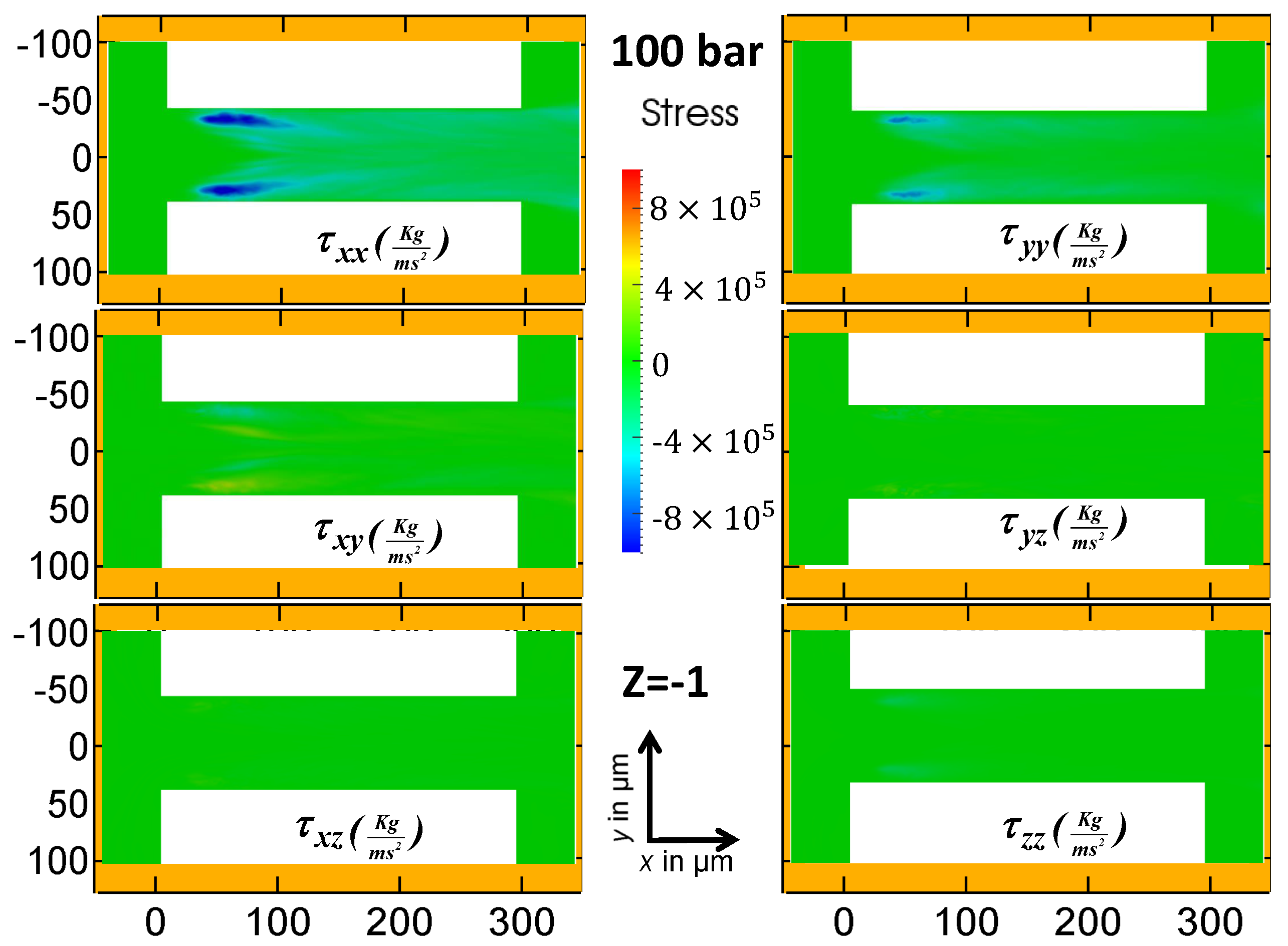
The laminar stresses produced in the orifice for the 100 bar and 500 bar cases in the mid-plane are shown in Figure 12 and Figure 13. The six independent stress components are depicted in each figure. In general, if the coordinate system is aligned with the flow direction, the diagonal components of the stress tensor cause a fluid element to be elongated. The diagonal components of the stress tensor in Figure 12 and Figure 13 are dominant. From the non-diagonal components, only has a significant contribution to the stress in the mid plane. However, the non-diagonal parts of the stress tensor become dominant closer to the wall, as depicted in Figure 14.
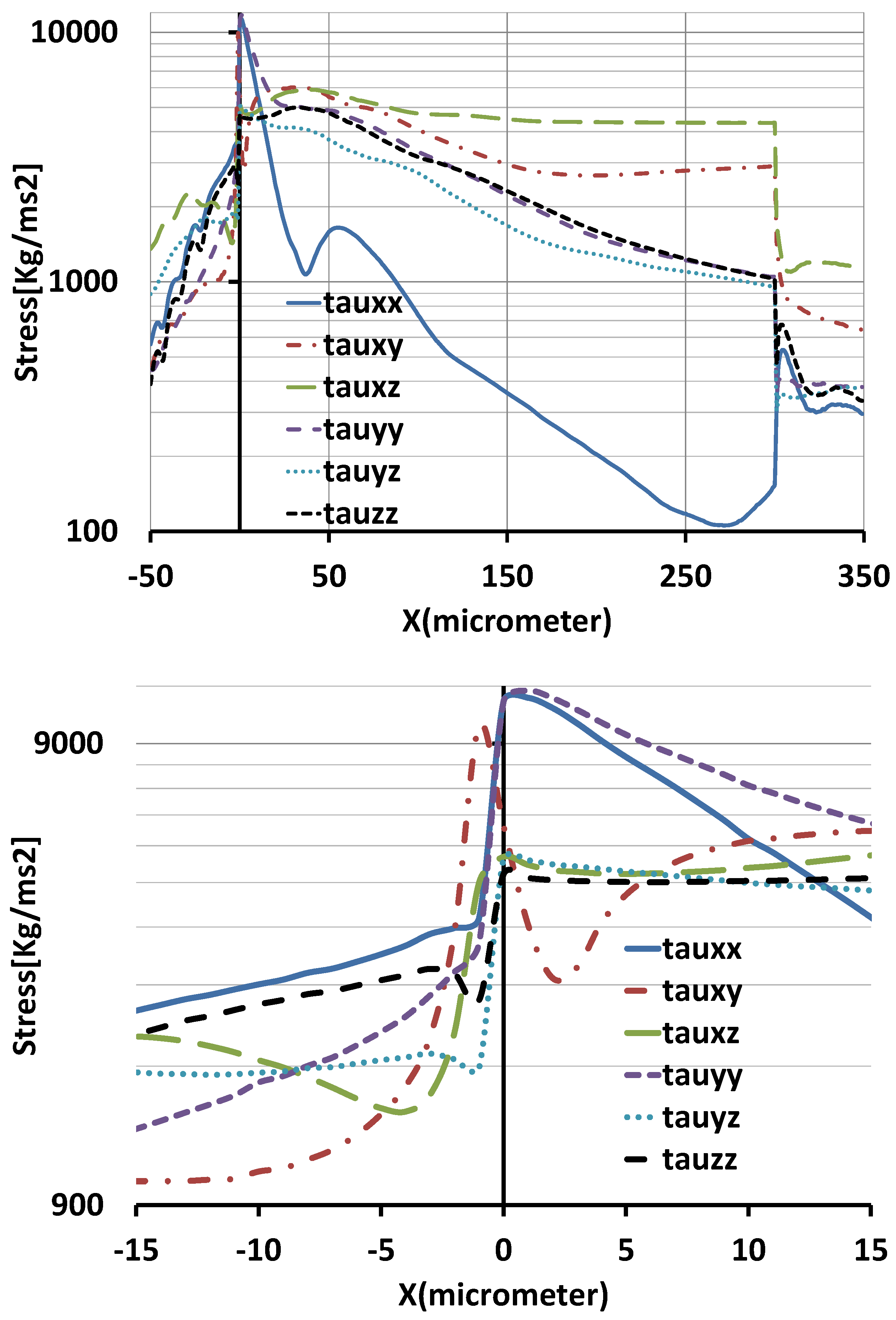
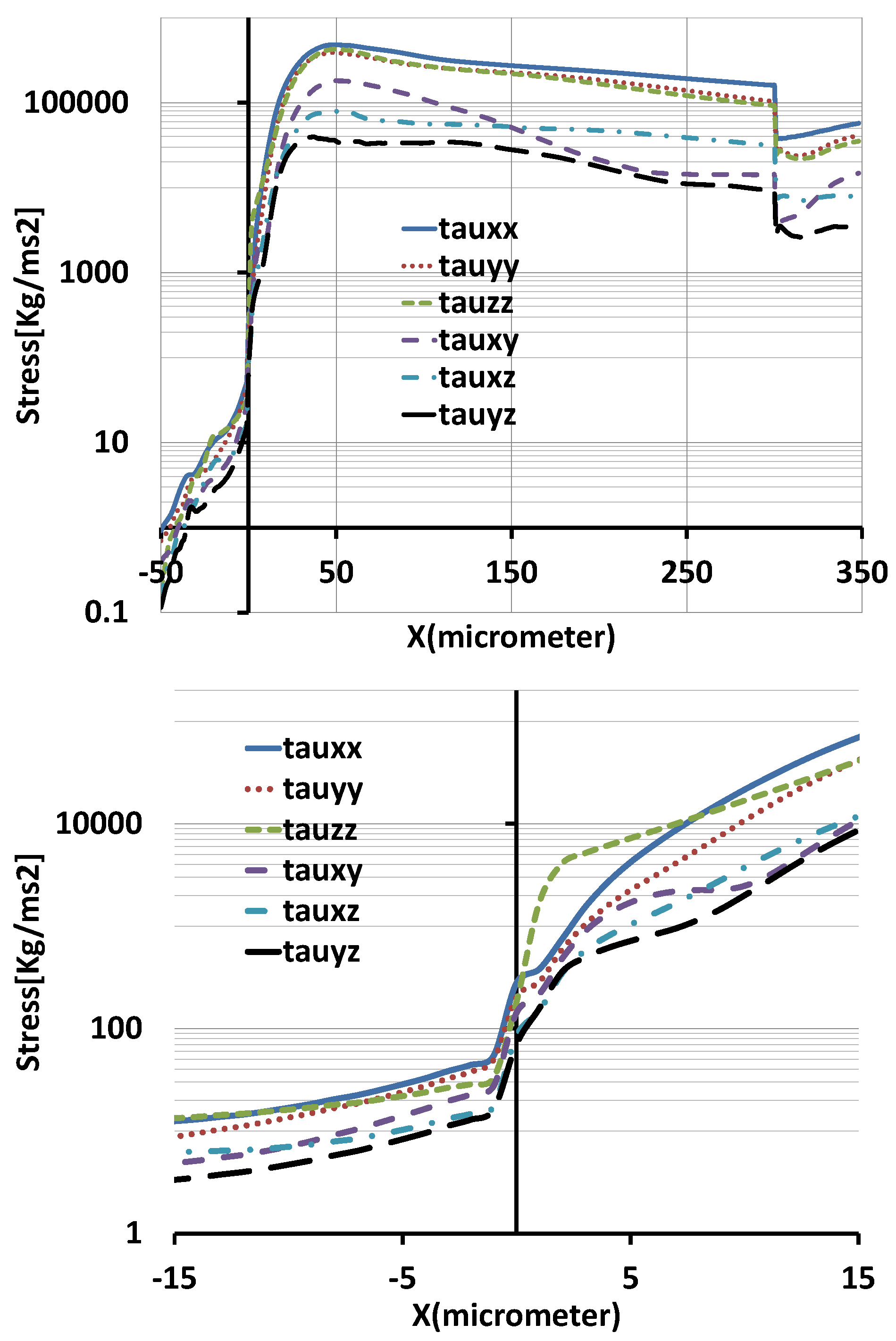
In order to quantitatively compare the effects of each stress component, the magnitude of the stress is averaged over planes and plotted along the length of the orifice (Figure 15). The upper figure shows the stress components from 50 μm before to 50 μm after the orifice. The lower figure shows a close-up of the upper figure. At the entrance, the diagonal components of the stress tensor and are dominant. The stress component decreases along the orifice. The stress component shows a complicated behavior. It starts from a low value and reaches its maximum a short distance in front of the entrance. After a short distance from the entrance, it reaches a local minimum.
The components of the turbulent stress tensor for the 100 bar and 500 bar cases are shown in Figure 16 and Figure 17. These figures are taken in the mid-plane of the orifice. The trace of the turbulent stress tensor constitutes the turbulent kinetic energy of the fluid flow. The magnitude of the diagonal components is considerably larger than the non-diagonal components in the mid-plane. As for the laminar stresses, only has a significant contribution among the non-diagonal stresses.
Unlike the laminar stresses, turbulent stresses play no role at the entrance of the orifice. The turbulence is produced where the laminar stresses are high, and moves downstream with the flow. The turbulent flow near the wall in the plane is shown in Figure 18. The values for the turbulent stresses are seen to be smaller close to the wall than in the mid-plane. The diagonal components of the turbulent stress tensor are dominant before, after, and inside of the orifice. This behavior can be seen in Figure 19. The upper figure shows the average magnitude of the turbulence stress for each component. The lower figure is a close-up of the upper figure.
The maximum of the turbulent stress is observed where the velocity obtains its peak value at about 50 μm behind the entrance of the orifice.
From comparing the turbulent stress in Figure 19 to the laminar stress in Figure 15, we see that the turbulent stress is generally one order of magnitude larger than the maximum of the laminar stress. Our result is therefore in disagreement with the result by Beinert et al. [49], who simulated the same device at the same pressure drop values and obtained turbulent stresses one order of magnitude larger than we did while simultaneously reporting laminar stresses one order of magnitude lower than ours. This difference merits some further discussion. Beinert et al. obtained their result by applying the commercial software ANSYS Fluent 14.0 using a Reynolds-stress model. The turbulent stresses in this software are obtained from empirical closure relations, which are not primarily designed to obtain microscopic stresses. Their approach is therefore based on the assumption that the modeled Reynolds-stresses are valid substitutes of the turbulent stresses. On the other hand, our approach does not rely on explicit turbulence models. The turbulent stresses in our model are essentially obtained by direct simulation of the Navier–Stokes equation. Yet, this does not prove that our result is correct. In order to check for the plausibility of their result, Beinert et al. estimated the size of the eddies necessary to comply with the stresses obtained from their turbulence model. For this, they had to estimate the velocity at which the eddy rotates; they chose the maximum velocity measured in the flow, which they give as 250 m/s for the case of 200 bar (we obtained a similar maximum velocity). With this, they obtained eddy sizes of 154 nm. This was compared to an estimate of the Kolmogorov scale obtained from the dissipation, which was estimated as , with m/s being the maximal velocity observed in the flow and l being the size of the largest eddies, corresponding to the diameter of the orifice. Under those assumptions, the Kolmogorov scale was estimated to be 33 nm, which was judged to be sufficiently smaller than the smallest estimated eddy size computed from the Reynolds-stress model to support the validity of their result. As our result for the same test case was different, we have re-examined this procedure. First of all, the hypothesis that the smallest eddies would rotate with a velocity equal to the global maximum in the flow does not appear to be very plausible. It should be noted that the argument depends crucially on this point, as the size of the smallest eddies required for their dissipation is inversely proportional to the assumed velocity. Under the assumption that the velocity of the smallest eddies would be five times smaller than the global maximum, the obtained eddies would already be smaller than the Kolmogorov length scale, which would render the results unphysical according to the criterion of Beinert et al. Another crucial point is that the estimates of Beinert et al. require that the smallest eddies are responsible for the largest stress, which is also only plausible under the assumption that the velocity of the smallest eddies was very high. Now we return to our own results and try to estimate Kolmogorov length. The Kolmogorov length is computed from the turbulent dissipation and the kinematic viscosity of water as:
The dissipation in the orifice according to our results is depicted in Figure 8. If we pick, e.g., a value of for the 100 bar case, we obtain a Kolmogorov scale of nm, which is three times smaller than the smallest grid spacing in our simulation. In order to check the plausibility of this value, we also estimate the dissipation in another way. The global energy dissipation of the flow in the device is easily obtained from the measurement in Figure 3. It is calculated as the volume flux times the pressure drop; i.e., W for the 100 bar case. In order to compute the dissipation rate, we have to specify a volume in which the dissipation takes place. Here we assume that all dissipation is confined to the orifice, which gives us:
We see that this value is six times larger than the dissipation obtained directly from the simulation. This rough estimate neglects the fact that the jet behind the orifice participates in the dissipation, and that the remainder of the device is 30 times larger than the orifice itself. This estimate must therefore over-predict the real dissipation, which is compatible with the observation that the previous estimate is smaller. The corresponding Kolmogorov length obtained from this estimate is expected to under-predict the the real Kolmogorov scale. We obtain nm. Note in particular that the last estimate of the Kolmogorov length was obtained entirely from the experimentally-measured flow rate, and did not use any data obtained from the simulation. The so-obtained Kolmogorov length—which underpredicts the real Kolmogorov length—is larger than the one estimated by Beinert et al. Thus, we conclude that the turbulent stresses and the associated dissipation rate is physically more plausible than the results obtained by Beinert et al.
5. Conclusions
We used a high-fidelity implicit large eddy simulation code based on the cumulant lattice Boltzmann method to simulate the turbulent flow through a mirco-orifice. In this paper, we especially focused on turbulent quantities like turbulent stresses and dissipation. In particular, we compare our results to the state-of-the-art approach to obtain turbulent stresses from the empirical Reynolds-stresses of standard turbulence models. It is found that our results for turbulent stresses disagree with published results obtained from RANS equations. The plausibility of our results is checked with the Kolmogorov theory, and it is found that the RANS model predictions for the smallest eddy sizes appear inconsistent. We conclude that our approach of a direct simulation without an explicit turbulence model is a priori more sound in terms of the underlying physics of the problem considered. The resolution in our simulation could support eddies up to about three times the Kolmogorov size, such that it can be considered as a very highly resolved LES. It is not possible to obtain turbulent shear stresses from experiments directly such that time- and space-resolved simulations such as the ones presented here are the only practical means to check the plausibility of RANS results in this regard. Since such resolved simulations are very expensive in terms of compute time, the results from RANS models are rarely challenged. Here we observed a clear indication that standard RANS turbulence models might have deficiencies in obtaining quantitative turbulent stresses for the problem class under consideration.
Acknowledgments
We thank the Deutsche Forschungsgemeinschaft for financial support of the research training group FOR 856 under fund number GE 1990/3-1.
Author Contributions
E.K.F. conducted the simulations and analyzed the results. M.G. developed the computational model and assisted in writing the paper. K.K. implemented larges parts of the simulation software. M.K. contributed in the computational setup and analysis of the results.
Conflicts of Interest
The authors declare no conflict of interest.
References
- Husain, Z.D. Theoretical Uncertainty of Orifice Flow Measurement. In Proceedings of the International School of Hydrocarbon Measurement, Oklahoma City, OK, USA, 16–18 May 1995; pp. 70–75. [Google Scholar]
- McCabe, W.L.; Smith, J.C.; Harriott, P. Unit Operations of Chemical Engineering; McGraw-Hill: New Delhi, India, 2005; p. 1140. [Google Scholar]
- Doblhoff-Dier, K.; Kudlaty, K.; Wiesinger, M.; Gröschl, M. Time resolved measurement of pulsating flow using orifices. Flow Meas. Instrum. 2011, 22, 97–103. [Google Scholar] [CrossRef]
- Peters, F.; Groß, T. Flow rate measurement by an orifice in a slowly reciprocating gas flow. Flow Meas. Instrum. 2011, 22, 81–85. [Google Scholar] [CrossRef]
- Baker, R.C. Flow Measurement Handbook: Industrial Designs, Operating Principles, Performance, and Applications; Cambridge University Press: Cambridge, UK, 2000; p. 95. [Google Scholar]
- Gallagher, J.E. Natural Gas Measurement Handbook; Gulf Publishing Company: Houston, TX, USA, 2006; p. 468. [Google Scholar]
- Cristancho, D.E.; Coy, L.A.; Hall, K.R.; Iglesias-Silva, G.A. An alternative formulation of the standard orifice equation for natural gas. Flow Meas. Instrum. 2010, 21, 299–301. [Google Scholar] [CrossRef]
- Åman, R.; Handroos, H.; Eskola, T. Computationally efficient two-regime flow orifice model for real-time simulation. Simul. Model. Pract. Theor. 2008, 16, 945–961. [Google Scholar] [CrossRef]
- Graves, D. Effects of Abnormal Conditions on Accuracy of Orifice Measurement. Pipeline Gas J. 2010, 237, 35–37. [Google Scholar]
- Gothsch, T.; Finke, J.H.; Beinert, S.; Lesche, C.; Schur, J.; Büttgenbach, S.; Müller-Goymann, C.; Kwade, A. Effect of microchannel geometry on high-pressure dispersion and emulsification. Chem. Engin. Technol. 2011, 34, 335–343. [Google Scholar] [CrossRef]
- Gothsch, T.; Schilcher, C.; Richter, C.; Beinert, S.; Dietzel, A.; Büttgenbach, S.; Kwade, A. High-pressure microfluidic systems (HPMS): Flow and cavitation measurements in supported silicon microsystems. Microfluid. Nanofluid. 2015, 18, 121–130. [Google Scholar] [CrossRef]
- Chen, D.; Cui, B.; Zhu, Z. Numerical simulations for swirlmeter on flow fields and metrological performance. Trans. Inst. Meas. Control 2016, in press. [Google Scholar] [CrossRef]
- Eiamsa-Ard, S.; Ridluan, A.; Somravysin, P.; Promvonge, P. Numerical investigation of turbulent flow through a circular orific. KMITL Sci. J. 2008, 8, 43–50. [Google Scholar]
- Shah, M.S.; Joshi, J.B.; Kalsi, A.S.; Prasad, C.; Shukla, D.S. Analysis of flow through an orifice meter: CFD simulation. Chem. Eng. Sci. 2012, 71, 300–309. [Google Scholar] [CrossRef]
- Reader-Harris, M.; Barton, N.; Hodges, D. The effect of contaminated orifice plates on the discharge coefficient. Flow Meas. Instrum. 2012, 25, 2–7. [Google Scholar] [CrossRef]
- Nakao, M.; Kawashima, K.; Kagawa, T. Measurement-integrated simulation of wall pressure measurements using a turbulent model for analyzing oscillating orifice flow in a circular pipe. Comput. Fluids 2011, 49, 188–196. [Google Scholar] [CrossRef]
- Gronych, T.; Jeřáb, M.; Peksa, L.; Wild, J.; Staněk, F.; Vičar, M. Experimental study of gas flow through a multi-opening orifice. Vacuum 2012, 86, 1759–1763. [Google Scholar] [CrossRef]
- Durst, F.; Wang, A.B. Experimental and numerical investigations of the axisymmetric, turbulent pipe flow over a wall-mounted thin obstacle. In Proceedings of the 7th Symposium on Turbulent Shear Flows, Stanford, CA, USA, 21–23 August 1989. [Google Scholar]
- Oliveira, N.M.; Vieira, L.G.; Damasceno, J.J.R. Numerical Methodology for Orifice Meter Calibration. Mater. Sci. Forum 2010, 660–661, 531–536. [Google Scholar] [CrossRef]
- Geier, M.; Schönherr, M.; Pasquali, A.; Krafczyk, M. The cumulant lattice Boltzmann equation in three dimensions: Theory and validation. Comput. Math. Appl. 2015, 70, 507–547. [Google Scholar] [CrossRef]
- Goraki Fard, E. A Cumulant LBM Approach for Large Eddy Simulation of Dispersion Microsystems. Ph.D. Thesis, TU Braunschweig, Braunschweig, Germany, 2015. [Google Scholar]
- Kian Far, E.; Geier, M.; Kutscher, K.; Krafczyk, M. Distributed cumulant lattice Boltzmann simulation of the dispersion process of ceramic agglomerates. J. Comput. Methods Sci. Eng. 2016, 16, 231–252. [Google Scholar] [CrossRef]
- Far, E.K.; Geier, M.; Kutscher, K.; Krafczyk, M. Simulation of micro aggregate breakage in turbulent flows by the cumulant lattice Boltzmann method. Comput. Fluids 2016, 140, 222–231. [Google Scholar] [CrossRef]
- Richter, C.; Krah, T.; Büttgenbach, S. Novel 3D manufacturing method combining microelectrial discharge machining and electrochemical polishing. Microsyst. Technol. 2012, 18, 1109–1118. [Google Scholar] [CrossRef]
- Geier, M.; Greiner, A.; Korvink, J.G. A factorized central moment lattice Boltzmann method. Eur. Phys. J. Spec. Top. 2009, 171, 55–61. [Google Scholar] [CrossRef]
- Geier, M.; Greiner, A.; Korvink, J.G. Bubble functions for the lattice Boltzmann method and their application to grid refinement. Eur. Phys. J. Spec. Top. 2009, 171, 173–179. [Google Scholar] [CrossRef]
- Schönherr, M.; Kucher, K.; Geier, M.; Stiebler, M.; Freudiger, S.; Krafczyk, M. Multi-thread implementations of the lattice Boltzmann method on non-uniform grids for CPUs and GPUs. Comput. Math. Appl. 2011, 61, 3730–3743. [Google Scholar] [CrossRef]
- Geier, M.; Schönherr, M. Esoteric Twist: An Efficient in-Place Streaming Algorithmus for the Lattice Boltzmann Method on Massively Parallel Hardware. Computation 2017, 5, 19. [Google Scholar] [CrossRef]
- Gong, Y.; Tanner, F.X. Comparison of RANS and LES Models in the Laminar Limit for a Flow over a Backward-Facing Step Using OpenFOAM. In Proceedings of the Nineteenth International Multidimensional Engine Modeling Meeting at the SAE Congress, Detroit, MI, USA, 19 April 2009. [Google Scholar]
- Munson, B.R.; Young, D.F.; Okiishi, T. Fundamentals of Fluid Mechanics, 4th ed.; John Wiley and Sons: Hoboken, NJ, USA, 2006; p. 481. [Google Scholar]
- Streeter, V.L. Handbook of Fluid Dynamics; McGraw-Hill: New York, NY, USA, 1961; p. 413. [Google Scholar]
- Kähler, G.; Bonelli, F.; Gonnella, G.; Lamura, A. Cavitation inception of a van der Waals fluid at a sack-wall obstacle. Phys. Fluids 2015, 27, 123307. [Google Scholar] [CrossRef]
- Shaaban, S. Optimization of orifice meter’s energy consumption. Chem. Eng. Res. Des. 2014, 92, 1005–1015. [Google Scholar] [CrossRef]
- Munson, B.R.; Young, D.F. Fundamentals of Fluid Mechanics, 5th ed.; John Wiley and Sons: Hoboken, NJ, USA, 2009; p. 481. [Google Scholar]
- Blasius, H. Das ähnlichkeitsgesetz bei reibungsvorgängen in flüssigkeiten. In Mitteilungen Über Forschungsarbeiten Auf Dem Gebiete Des Ingenieurwesens; Springer: Berlin/Heidelberg, Germany, 1913; pp. 1–41. (In German) [Google Scholar]
- Fluent, A. ANSYS Fluent 12.0 User’s Guide; ANSYS Inc.: Canonsburg, PA, USA, 2009; p. 48. [Google Scholar]
- Shur, M.L.; Strelets, M.K.; Travin, A.K.; Spalart, P.R. Turbulence modeling in rotating and curved channels: Assessing the Spalart-Shur correction. AIAA J. 2000, 38, 784–792. [Google Scholar] [CrossRef]
- Schumann, U. Realizability of Reynolds-Stress Turbulence Models. Phys. Fluids 1977, 20, 721. [Google Scholar] [CrossRef]
- Haller, G. An objective definition of a vortex. J. Fluid Mech. 2005, 525, 1–26. [Google Scholar] [CrossRef]
- Green, M.A.; Rowley, C.W.; Haller, G. Detection of Lagrangian Coherent Structures in Three-Dimensional Turbulence. J. Fluid Mech. 2007, 572, 111. [Google Scholar] [CrossRef]
- Dubief, Y.; Delcayre, F. On coherent-vortex identification in turbulence. J. Turbul. 2000, 1, 11. [Google Scholar] [CrossRef]
- Chakraborty, P.; Balachandar, S.; Adrian, R.J. On the relationships between local vortex identification schemes. J. Fluid Mech. 2005, 535, 189–214. [Google Scholar] [CrossRef]
- Hunt, J.C.R.; Wray, A.A.; Moin, P. Eddies, streams, and convergence zones in turbulent flows. In Proceedings of the Summer Program on Studying Turbulence Using Numerical Simulation Databases, Stanford, CA, USA, 27 June–22 July 1988; pp. 193–208. [Google Scholar]
- Kuo, K.K.; Acharya, R. Fundamentals of Turbulent and Multiphase Combustion; John Wiley & Sons, Inc.: Hoboken, NJ, USA, 2012; p. 220. [Google Scholar]
- Landahl, M.T.; Mollo-Christensen, E. Turbulence and Random Processes in Fluid Mechanics; Cambridge University Press: Cambridge, UK, 1992; p. 45. [Google Scholar]
- Tennekes, H.; Lumley, J.L. A First Course in Turbulence; MIT Press: Cambridge, MA, USA, 1972; p. 300. [Google Scholar]
- Fröhlich, J.; von Terzi, D. Hybrid LES/RANS methods for the simulation of turbulent flows. Prog. Aerosp. Sci. 2008, 44, 349–377. [Google Scholar]
- Blazek, J. Computational Fluid Dynamics: Principles and Applications; Elsevier: Amsterdam, The Netherlands, 2005; pp. 227–270. [Google Scholar]
- Beinert, S.; Gothsch, T.; Kwade, A. Numerical evaluation of stresses acting on particles in high-pressure microsystems using a Reynolds stress model. Chem. Eng. Sci. 2015, 123, 197–206. [Google Scholar] [CrossRef]
Figure 1.
A schematic of the micro-orifice meter.
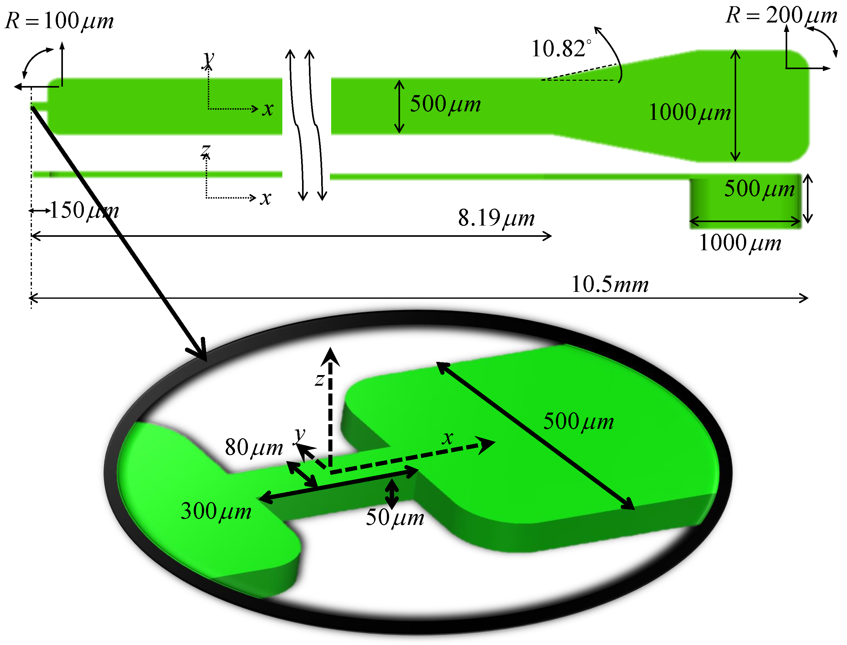
Figure 2.
Zoom into the grids at the orifice. Each block in the picture contains lattice nodes.

Figure 3.
Variation in flow rate with square root of pressure drop across orifice. Comparison between flow rates obtained by the LBM simulation and by experiment for the three pressure drops of 100 bar, 200 bar, and 500 bar. LBM: lattice Boltzmann method.
Figure 3.
Variation in flow rate with square root of pressure drop across orifice. Comparison between flow rates obtained by the LBM simulation and by experiment for the three pressure drops of 100 bar, 200 bar, and 500 bar. LBM: lattice Boltzmann method.

Figure 4.
The upper figure shows an average of 40,000 time steps of the simulation of the device, corresponding to a real time interval of 24.5 microseconds at a pressure difference of 500 bar. The lower picture shows a zoom into the velocity field. The effect of the vena contracta is demonstrated.
Figure 4.
The upper figure shows an average of 40,000 time steps of the simulation of the device, corresponding to a real time interval of 24.5 microseconds at a pressure difference of 500 bar. The lower picture shows a zoom into the velocity field. The effect of the vena contracta is demonstrated.

Figure 5.
The center line magnitude velocity for three different pressure drops. The positions and μm coincide with the entrance and the exit of the orifice, respectively.
Figure 5.
The center line magnitude velocity for three different pressure drops. The positions and μm coincide with the entrance and the exit of the orifice, respectively.

Figure 6.
The time-averaged pressure for the 100 bar and 500 bar cases at two different planes. The upper picture for each set shows the pressure for plane μm, and the lower shows the pressure for μm. All pressure is measured relative to the pressure at the outlet.
Figure 6.
The time-averaged pressure for the 100 bar and 500 bar cases at two different planes. The upper picture for each set shows the pressure for plane μm, and the lower shows the pressure for μm. All pressure is measured relative to the pressure at the outlet.

Figure 7.
The time averaged pressure over z direction through the orifice for the 100 bar case and the 500 bar case. The positions and μm coincide with the entrance and the exit of the orifice, respectively. All pressure is measured relative to the pressure at the outlet.
Figure 7.
The time averaged pressure over z direction through the orifice for the 100 bar case and the 500 bar case. The positions and μm coincide with the entrance and the exit of the orifice, respectively. All pressure is measured relative to the pressure at the outlet.

Figure 8.
The logarithmic plot of the total dissipation rates versus x-direction for two pressure drops. The dissipation rates are averaged over the z direction. The position coincides with the orifice entrance.
Figure 8.
The logarithmic plot of the total dissipation rates versus x-direction for two pressure drops. The dissipation rates are averaged over the z direction. The position coincides with the orifice entrance.

Figure 9.
The Q-criterion for the time averaged flow through the device for the 100 bar case. The color shows the magnitude of the velocity.
Figure 9.
The Q-criterion for the time averaged flow through the device for the 100 bar case. The color shows the magnitude of the velocity.
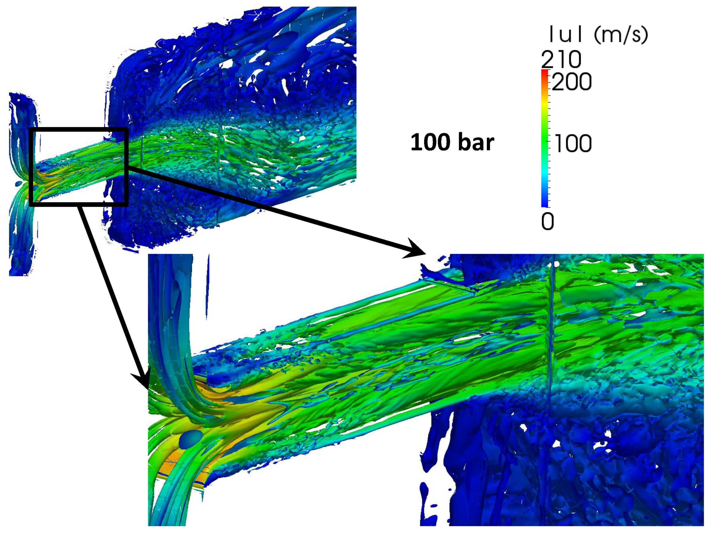
Figure 10.
The Q-criterion for the time-averaged flow through the device for the 200 bar case. The color shows the magnitude of the velocity.
Figure 10.
The Q-criterion for the time-averaged flow through the device for the 200 bar case. The color shows the magnitude of the velocity.
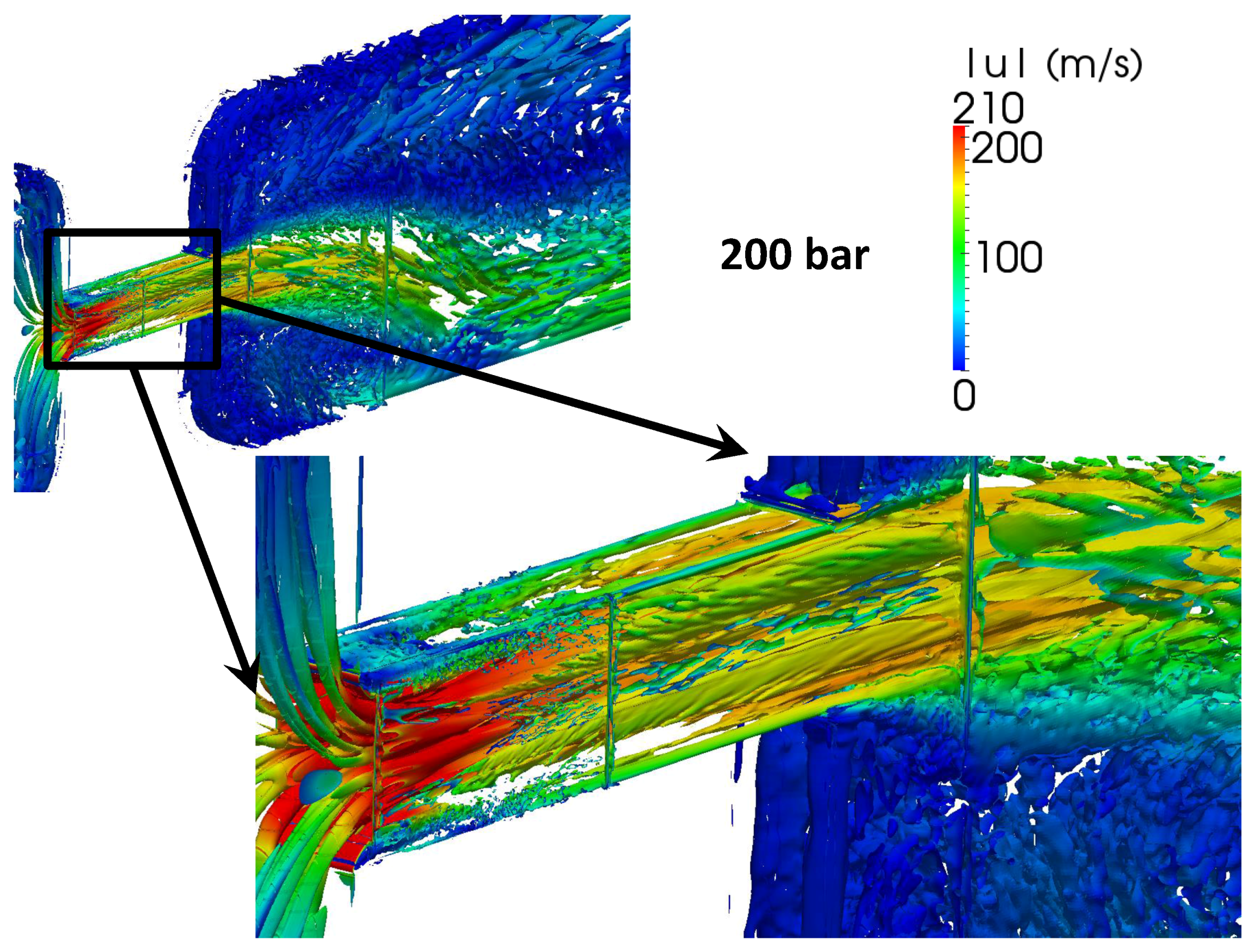
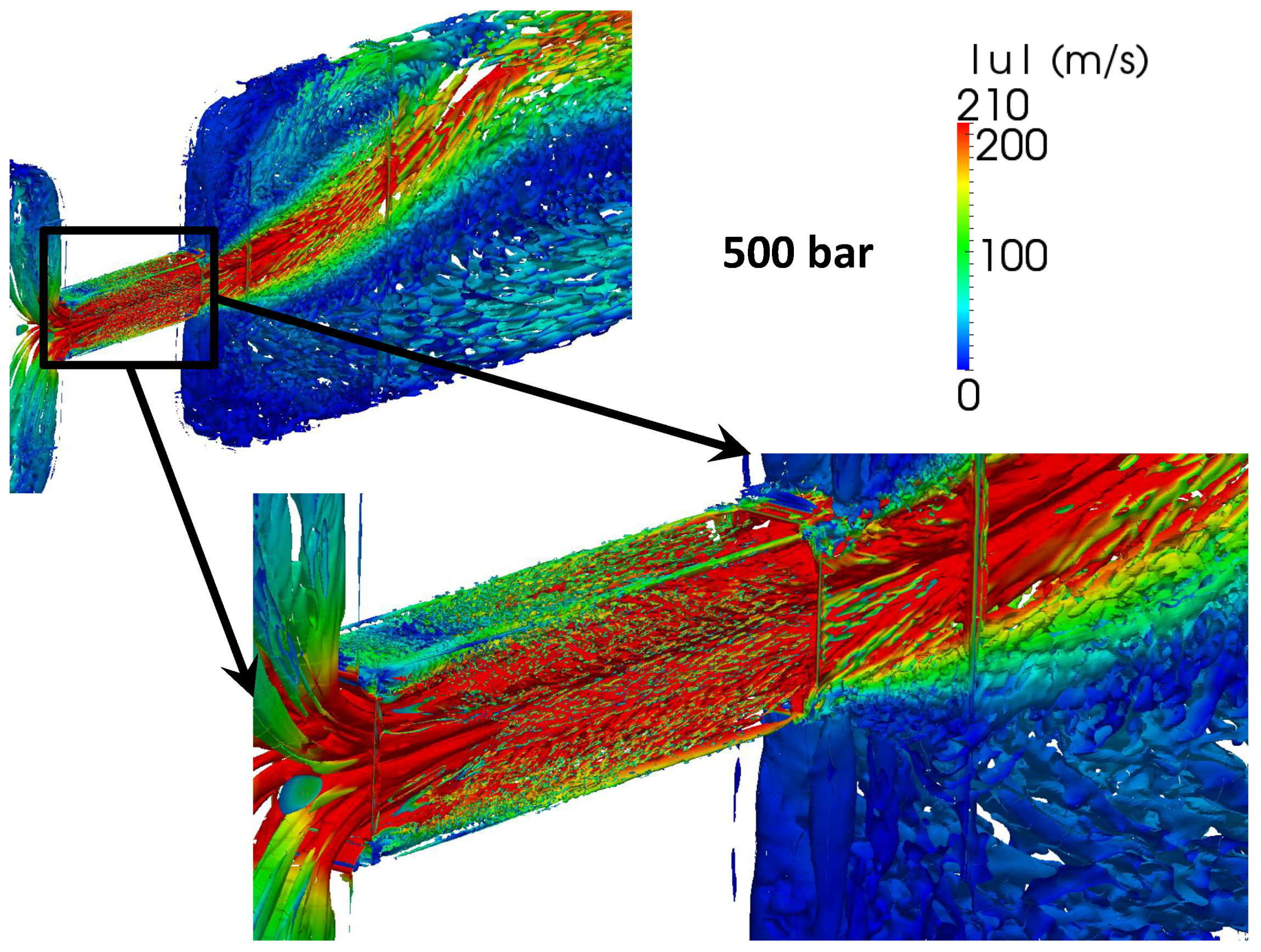
Figure 11.
The Q-criterion for the time averaged flow through the device for the 500 bar case. The color shows the magnitude of the velocity.
Figure 11.
The Q-criterion for the time averaged flow through the device for the 500 bar case. The color shows the magnitude of the velocity.

Figure 12.
The laminar stress components generated in the orifice in the mid plane for a pressure drop of 100 bar.
Figure 12.
The laminar stress components generated in the orifice in the mid plane for a pressure drop of 100 bar.

Figure 13.
The laminar stress components generated in the orifice in the mid plane for a pressure drop of 500 bar.
Figure 13.
The laminar stress components generated in the orifice in the mid plane for a pressure drop of 500 bar.

Figure 14.
The laminar stress components generated in the orifice in the plane for a pressure drop of 100 bar.
Figure 14.
The laminar stress components generated in the orifice in the plane for a pressure drop of 100 bar.

Figure 15.
The laminar stress components averaged over the planes plotted in the x direction for a pressure drop of 100 bar. The upper figure shows the stress components from 50 μm before to 50 μm after the orifice. The lower figure shows a close-up of the upper figure.
Figure 15.
The laminar stress components averaged over the planes plotted in the x direction for a pressure drop of 100 bar. The upper figure shows the stress components from 50 μm before to 50 μm after the orifice. The lower figure shows a close-up of the upper figure.

Figure 16.
The turbulent stress components generated in the orifice in the mid-plane for a pressure drop of 100 bar.
Figure 16.
The turbulent stress components generated in the orifice in the mid-plane for a pressure drop of 100 bar.

Figure 17.
The turbulent stress components generated in the orifice in the mid-plane for a pressure drop of 500 bar.
Figure 17.
The turbulent stress components generated in the orifice in the mid-plane for a pressure drop of 500 bar.

Figure 18.
The averaged stress components generated in the orifice in the plane for the pressure drop of 100 bar.
Figure 18.
The averaged stress components generated in the orifice in the plane for the pressure drop of 100 bar.

Figure 19.
The turbulent stress components averaged over planes plotted in the x direction for a pressure drop of 100 bar. The upper figure shows the average magnitude of the turbulence stress for each component. The lower figure is a close-up of the upper figure.
Figure 19.
The turbulent stress components averaged over planes plotted in the x direction for a pressure drop of 100 bar. The upper figure shows the average magnitude of the turbulence stress for each component. The lower figure is a close-up of the upper figure.

© 2017 by the authors. Licensee MDPI, Basel, Switzerland. This article is an open access article distributed under the terms and conditions of the Creative Commons Attribution (CC BY) license (http://creativecommons.org/licenses/by/4.0/).
Share and Cite
MDPI and ACS Style
Kian Far, E.; Geier, M.; Kutscher, K.; Krafczyk, M. Implicit Large Eddy Simulation of Flow in a Micro-Orifice with the Cumulant Lattice Boltzmann Method. Computation 2017, 5, 23. https://doi.org/10.3390/computation5020023
AMA Style
Kian Far E, Geier M, Kutscher K, Krafczyk M. Implicit Large Eddy Simulation of Flow in a Micro-Orifice with the Cumulant Lattice Boltzmann Method. Computation. 2017; 5(2):23. https://doi.org/10.3390/computation5020023
Chicago/Turabian StyleKian Far, Ehsan, Martin Geier, Konstantin Kutscher, and Manfred Krafczyk. 2017. "Implicit Large Eddy Simulation of Flow in a Micro-Orifice with the Cumulant Lattice Boltzmann Method" Computation 5, no. 2: 23. https://doi.org/10.3390/computation5020023
Note that from the first issue of 2016, this journal uses article numbers instead of page numbers. See further details here.