1. Introduction
Vocalized speech is commonly considered to be the basic and the most natural means of daily communication between humans. As expected, many research efforts have turned to practical applications of voice user interfaces (VUIs) in human-machine interaction. Speech is considered to be a very complex signal, since apart from the meaning it carries information regarding the speaker’s identity and language and his/her emotion. Towards a natural voice interaction between a human and a computer, two basic aspects need to be tackled. The first is the recognition of the spoken content and the second is the recognition of the user’s emotion during the interaction. During the last years, emotion recognition from speech has constituted a very popular research area and many efforts aim to recognize a human’s emotional state solely from his/her speech.
Emotion recognition is usually more easily recognized through other channels, rather than the audio one. For example, a human’s gaze [
1], facial features [
2], gestures [
3] and even his/her pose [
4] may be in some cases more appropriate for this task, while physiological parameters e.g., photoplethysmogram, electromyogram, electrocardiogram etc. [
5] have also been successfully applied. However, in many cases visual information is either unavailable or insufficient, while physiological information typically requires specialized and obtrusive equipment. Thus speech may be the only available modality for emotion recognition.
When the type of the information is considered, we may divide the methods that adopt speech into two distinct categories [
6,
7]:
explicit or linguistic information, which concerns articulated patterns by the speaker; and
implicit or paralinguistic information, which concerns the variation in pronunciation of the linguistic patterns. Typical approaches that fall into the first category make use of an ASR system. On the other hand, paralinguistic approaches ignore the content of speech and instead focus on associating low-level features to emotions. Extracted features may either be low-level descriptors or statistics extracted on these descriptors.
Regardless of whether either one type of information is being used separately or the two types are being fused, one may attempt to classify a vocal signal that consists of speech based on its inherent emotion(s), which of course poses a significantly difficult task even for a human expert (e.g., a psychologist). One should expect that fusion approaches would have an advantage in terms of performance. Even when this is the case, we may argue that their disadvantages may in some cases render them non-practical. More specifically, their main disadvantage is that they do not typically provide a language-independent model. Each language has its own specifics and is subject to cultural differences. As such, there might exist a plethora of different sentences, speakers, speaking styles and rates [
8]. Thus research using linguistic features has mainly focused on multilingual emotion recognition. On the other hand, when tackling the task of language-independent emotion recognition, the most appealing approach is to use paralinguistic information.
Typical approaches extract a set of “hand-crafted” features, i.e., statistics of short-term feature vectors computed either on the time domain or the spectral/cepstral domain. Then supervised machine learning algorithms are trained on annotated data. Therein lies the most important drawback of these approaches: these features are computationally expensive. In this work we aim to present an approach, using deep neural networks that does not require any hand-crafted features in the process. During the last few years they have become a new trend in the field of machine learning having as their main advantage over traditional approaches that they do not need to be trained using specific features. Instead, they translate raw data into compact intermediate representations, while they remove any redundancy. Our approach relies on a Convolutional Neural Network (CNN) and we show that it is indeed able to replace the traditional approach of feature extraction, model training and classification and render paralinguistic features obsolete. Moreover, at an attempt to provide a language-independent approach, we use cross-language datasets.
The remaining of this paper is as follows: In
Section 2 we present related work within the broader research area of emotion recognition from multimedia, focusing on speech-based approaches. Moreover, emphasis is given on applications that rely on deep learning. Then, in
Section 3 we provide the theoretical background of the convolutional neural networks. In
Section 4 we present the training dataset and the augmentation process applied. In
Section 5 we present in detail the proposed approach. Experimental results are presented in
Section 6. Finally, we discuss our results and draw our conclusions in
Section 7, where we also present plans for future work and possible extensions of our approach.
2. Related Work
Emotion recognition approaches typically extract some low-level features and a machine learning approach is then used to map them to emotion classes. Such an approach is the one of Shen et al. [
9] who used support vector machines and features such as energy, pitch, Linear Prediction Cepstrum Coefficients (LPCC) and Mel Frequency Cepstrum Coefficients (MFCC) and showed that some emotions may be classified more effectively than others. Similarly, Kishore et al. [
10] extracted MFCC and wavelet features and used Gaussian Mixture Models. They showed that the latter may lead to improved performance, however none produces adequate results, thus other features or a fusion scheme may be needed. Several works proposed the use of other types of features, e.g., Yang and Lugger [
11] proposed harmony features. Moreover, Wu et al. [
12] proposed modulation spectral features. Bitouk et al. [
13] proposed the use of phoneme class MFCC and showed that traditional prosodic features and statistics of MFCC are outperformed. Moreover, their results indicated that spectral features from consonants may outperform the ones of vowels. Other approaches investigated combinations of features, such as the one of Koolagudi and Rao [
14] who used global and local prosodic features and developed emotion recognition models using each feature separately, or combinations of features. Their experiments indicated that features may work in a complementary fashion towards higher recognition performance. A fusion approach was presented by Wu et al. [
15], based on multiple classifiers. They used acoustic-prosodic information from emotional-salient segments which were initially detected from raw speech and combined this information with semantic labels which were extracted from recognized words and emotion association rules. They concluded that such rules are not easy to be defined and showed that classification based solely on acoustic and prosodic features may provide comparable performance.
Of course, traditional classification schemes still became insufficient and more complex ones were presented. An example is the work of Giannoulis and Potamianos [
16] who presented an approach that focused on classification between pairs of emotions and a feature selection scheme. They used prosodic, spectral, glottal and AM-FM features and a set of 15 binary classifier systems to detect 6 emotions using a voting approach and incorporated gender information. They showed that different features should be selected for every classifier. Lee et al. [
17] applied a hierarchical binary decision tree on several acoustic features. They placed the more easy problem at the top levels to ensure that accumulated errors shall be minimized. However, they introduced some heuristics within the process, which do not generalize to other datasets. Finally, Chen et al. [
18] proposed a three-level model, for pairwise classification and examined the use of several classifiers, showing that several emotions are still hard to detect.
Within the emotion recognition process there also several other issues that need to be tackled. The speaker’s gender plays a significant role, since both genders have significantly different vocal features and may express their emotions differently. At an attempt to investigate such issues, Bisio et al. [
19] demonstrated that the a-priori knowledge of gender may lead to a significant increase of performance, thus they proposed a system whose initial step was to classify the speaker’s gender based on spectral features of her/his voice. Typical recognition schemes work with utterances. However, Koolagudi et al. [
20] further segmented the speech signal into words and syllables and showed that by combining spectral and prosodic features, accuracy may be improved. Typical datasets use a studio environment, i.e., one without noise. Of course, noise may be present in practical applications and its effects may be severe. Tawari and Trivedi [
21] dealt with the effect of noise within a car environment and proposed an adaptive noise cancellation scheme which significantly improved results. Another issue when using publicly available data sets is how to effectively combine them. Lefter et al. [
22] presented an approach where combinations of several datasets for training and testing were used. They examined the case where evaluation took place in unseen datasets and showed that in that case and the performance was significantly low, although there were a few exceptions. Another paradigm for working with combinations of datasets was the one of Schuller et al. [
23] who proposed approaches and strategies for mapping emotions from different datasets to common classes (i.e., to valence and arousal), for evaluation and also for normalization of the datasets. However they did not address the common problem of cultural differences between datasets.
During the last few years, many research efforts have focused on deep learning, which is a class of machine learning algorithms that uses complex architectures of many interconnected layers, each consisting of nonlinear processing units. Each unit extracts and transforms features. Each layer’s input is the output of the previous one. Deep learning networks are able to learn multiple levels of representations of data. Their main advantage is that they do not need hand-crafted features, i.e., features that are extracted from raw data using specialized algorithms. Instead, features are learned from raw data and typically lead to higher performance. Of course, this is achieved with the cost of higher computational time. Several deep learning machines and architectures have been successfully applied towards emotion recognition from speech. For example, Stuhlsatz et al. [
24] used deep neural networks and generalized discriminant analysis and demonstrated superior performance over traditional features and classifiers. Han et al. [
25] first applied deep neural networks to compute probability distributions for each speech segment and for each emotion state. Then features were constructed from these distributions and used as input to an extreme learning machine. They showed that this way performance may be significantly increased, compared to traditional approaches. Huang et al. [
26] used convolutional neural networks (CNNs) to learn salient features, adopting a two-stage process. They showed that even in complex and noisy environments, such learnt features were superior to traditional ones. Li et al. [
27] used deep neural network hidden Markov models (HMMs). They showed that performance may be significantly increased compared to gaussian mixture models and traditional HMMs. Trigeorgis et al. [
28] combined CNNs with long short-term memory networks (LSTMs) and avoided the extraction of hand-crafted features, while performance was increased. Poria et al. [
29] presented a multimodal approach combining visual, audio and textual modalities using deep CNNs. The extracted features were then fed to a multiple kernel learning classifier. They reported significant improvement compared to state-of-the art approaches. Finally and similarly to our approach, Zheng et al. [
30] used CNNs on audio spectrograms and also showed their superiority over hand-crafted features.
Finally, we should note that several surveys have been conducted during the last decade, aiming to systematically present research on the broader areas of emotion recognition from all aspects. Notable works are the one of Koolagudi and Rao [
31] which emphasizes on databases, the one of Anagnostopoulos et al. [
6] which focuses mainly on features and classifiers that are used and finally the one of of El Ayadi et al. [
8], which focuses on both.
3. Convolutional Neural Networks
Deep Learning approaches have dominated the last five years in the machine learning field by achieving breakthrough results in a vast variety of applications especially in the areas of Computer Vision [
32] and Speech Processing [
33,
34]. Through those years many different approaches and deep learning structures have been proposed with the most dominant being the Convolutional Neural Networks (CNNs). Convolutional Neural Networks can be considered as an alteration of traditional Neural Networks, where the goal of the training algorithm is to learn a set of convolutional filters by optimizing the classification error at output of the Network. In contrast to traditional ANNs, in a CNN the neurons in every layer are affected only by a sub-region of the previous layer without taking into consideration the pixel values of the whole image. Having that in mind, we can argue that CNNs are a very powerful mechanism, able to express computationally heavy models and robust feature representations, while keeping the number of tuning parameters relatively small. As every other Neural Network, CNNs may consist of an arbitrary number of layers, where each layer may have a different number of nodes. The learning process of a CNN is quite similar to every other Neural Network architecture, where a forward propagation of the data and a backward propagation of the error take place in order to update the weight parameters. Most common learning algorithms of such architectures are gradient-based with the most important being the Stochastic-Gradient-Descent and the Adaptive Gradient. CNN layers can be discriminated into four different categories, namely the (a) Convolutional Layers; (b) Pooling Layers; (c) Normalizing Layers; and the (d) Fully connected Layers.
Convolutional Layers are the key component of any CNN architecture. The most popular way of shaping a convolutional layer is by grouping neurons in a rectangular (most commonly squared) grid, whose parameters are learned during the training process. Rectangular neuron grids have been proven ideal for image processing tasks where the input data are naturally rectangular shaped. Even though in this work square grids of neurons are deployed, a convolutional layer may also consist of 1-D convolutional matrices. Every such matrix with , describes a convolutional filter. In our case, since rectangular filters are used, input and output of the convolutional layers should also be rectangular. The key characteristic of CNNs is that, the weights of the rectangular section that gets affected by the convolutional layer are the same for each neuron. Hence, those layers are just an image convolution of the previous layer, where the weights specify the convolution filter. In addition, there may be several grids in each convolutional layer; each grid takes inputs from all grids in the previous layer, using potentially different filter.
Pooling Layers are usually placed after a single or a set of serial or parallel convolutional layers. This layer type takes small rectangular blocks from the convolutional layer and subsamples it to produce a single output from that block. The necessity of pooling layers stems out of need to learn complex features, from different image resolutions while keeping the number of parameters and the computational cost as low as possible. In addition pooling layers act as a very effective mechanism to control over-fitting and increase the invariance of the learned model parameters.
Normalization Layers are intermediate layers responsible for data normalization and in some cases can lead to minor improvements on the final decision. Those layers are used for normalization over local input regions thus, increasing their discrimination ability over their neighbours.
Fully-Connected Layers are the top level layers of every CNN structure and are responsible for the high-level reasoning of the network. A fully connected layer takes all neurons in the previous layer (be it fully connected, pooling, or convolutional), connecting them to each of its single neurons. Fully connected layers are not spatially located anymore (you can visualize them as one-dimensional), so there can be no convolutional layers after a fully connected layer. The last fully-connected layer is always attached to a loss-function (SVM, Softmax, Euclidean Loss etc.) that is used to estimate the final classification error and is responsible for updating the network weights during the back-propagation.
One of the major drawbacks of deep-learning approaches are their inability to avoid over-fitting when the amount of available training data is limited, which is the case in most real life scenarios. Usually to train robust and generalized deep structures an amount of training samples in the order of tens of thousands is required. Several tricks have been proposed to alleviate the aforementioned problem and produce more descriptive features, with the most popular being the Dropout-Technique and the Input-Batch-Normalization.
The
Dropout Technique [
35] follows the very simple assumption that different feature combinations can represent different aspects of the scene that we wish to describe. Thus at each training stage, individual nodes are either ”dropped out” of the net with probability
or kept with probability
p so that a reduced network is left; incoming and outgoing edges to a dropped-out node are also removed. Only the reduced network is trained on the data in that stage and the removed nodes are reinserted into the network in the next stage with their original weights.
The
Input-Batch-Normalization Technique [
36] comes as a solution to two well known problems usually faced when training a deep architecture that can often lead to over-fitting or inability to achieve efficient learning. Those problems are the
Internal-Covariate-Shift, which refers to the change in the input distribution as it is affected by the parameters in all the input layers and the
Vanishing Gradient, where activation functions (such as tanh or sigmoid) tend to get stuck in the saturation region as the length of the network increases. Batch-Normalization transforms and scales every input dimension before it goes through the non-linearity. Assume
dimension of an input; we can normalise this dimension as :
After normalizing the input values, scaling and shifting should be applied in order to enable the layer to produce more generic representations, which will not be bounded strictly by the linear segments of the activation function. Thus the normalized imput is transformed to:
where
and
are learnable parameters.
The x to y transformation is called Batch-Normalization and is very powerful in reducing internal covariant shift and the dependence of gradients on the scale of the parameters. In addition it acts as a model regularization technique and allows the use of saturating non-linearities (like tanh or sigmoid) and higher learning rates.
4. Training Dataset and Augmentation
For our experiments we used four different audio datasets. Three of the datasets are publicly available (Emovo [
37], Savee [
38], German [
39]) and the last one is a custom made dataset, which includes audio samples gathered from movies. For the custom made dataset the samples were annotated manually by several researchers in NCSR Demokritos. All the movies used for creation of our Movies-Dataset were in English except one that was in Portuguese. Statistics of the aforementioned datasets are reported in
Table 1.
Since not all the datasets included samples for all the classes of
Table 1, we decided to work only on their union. Thus, our final dataset consists only of the five common classes, namely anger, fear, happiness, neutral and sadness.
Our CNN architecture (
Section 5) has been trained using a set of pre-segmented audio samples, randomly cropped from the original audio signal, each one belonging to any of the 5 classes (happiness, fear, sadness, anger, neutral) and with fixed duration equal to 2 s.
More specifically, we trained four different models, each time using samples from a single dataset. Each model was trained using the 80% of the samples from each class of the dataset. For evaluation purposes we performed four different experiments for each trained model (i.e., 16 experiments in total). We tested each trained model on the remaining 20% of samples from each class of the training dataset (note that those samples were used only for testing). Then we performed three additional experiments using each time all samples of each one of the other datasets.
As mentioned in
Section 3, deep learning techniques require huge amounts of training data, in order to achieve satisfactory classification performance rates and avoid over-fitting. In cases that the original data size is limited, as in our scenario, data augmentation is required to overcome this data scarcity problem. Data augmentation is defined as a series of deformations applied on the annotated training samples which results in new additional training data [
40]. In most computer vision applications that utilize deep learning for classification, data augmentation is achieved through image reformations such as horizontally flipping, random crops and color jittering. In our case, before extracting the spectrogram of each training sample we add a background sound (playing the role of noise) in three different Signal-To-Noise ratios (5, 4 and 3) for the crop of the original audio sample. If we also include the original (no noise) training sample, this means that this data augmentation procedure achieves a
dataset increase.
Figure 1 presents an example of two original (no noise) signals.
From each audio stream a single randomly cropped segment of 2 s length is extracted. For each segment, its spectrogram is extracted, using 40 ms short-term window size and 20 ms step. This spectrogram is the adopted representation for each 2-second segment of the audio stream, which is fed as input to the CNN, described in the next section.
5. Method
For recognising the five-target emotion labels, we utilized a CNN classifier (
CNN_EM) that operates upon the pseudocolored spectrogram images. As recent literature has shown, deep hierarchical visual feature extractors can significantly outperform shallow classifiers trained on hand-crafted features and are more robust and generalizable when countering problems that include significant levels of inherent noise. The architecture of our deep CNN structure was finalized after a very extensive experimentation process on different layer combinations and parameter tuning. Our goal was to build a model, that could depict robust feature representations for recognizing speech-emotion accross all the datasets, in a language independent manner. For our experiments we used the BVLC Caffe deep-learning framework [
41] (All Caffe trained models and necessary code to reproduce our experiments is available on Github:
https://github.com/MikeMpapa/CNNs-Audio-Emotion-Recognition).
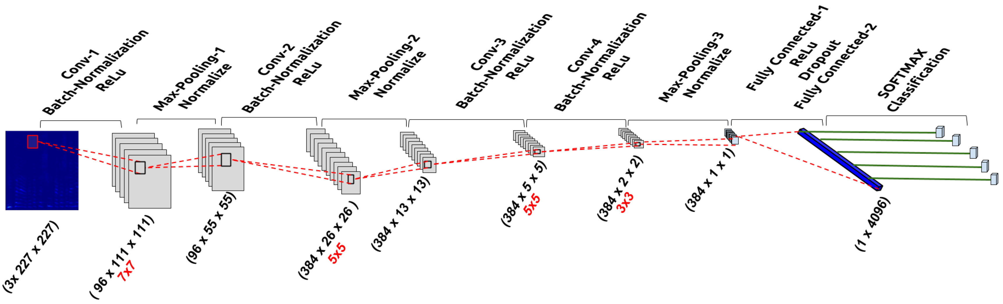
The network architecture consists of four convolution layers in total, all of them with a stride of 2. The kernel sizes of the convolutional layers are of size 7, 5, 5 and 3 respectively. After every convolution and before the application of the non-linearity function we normalize the input batch using the Batch-Normalization transformation described in
Section 3. In addition, in-between the initial three convolutional layers and after the last one, a pooling layer followed by a normalization layer is interposed. In this work, normalization layers adopt the LRN (Local Responce Normalization) normalization method and all max-pooling layers have a kernel with size equal to 3 and a stride of 2. The last two layers of the network are fully connected layers with dropout, followed by a softmax classifier, that shapes the final probability distribution. For all the layers we used the ReLu as our activation function and weights are always initialized using the
xavier [
42] initialization. For the learning algorithm we decided to use the standard SGD, as it lead to superior results compared to other learning algorithms. The output of the network is a distribution on the five target classes, while the output vector of the final fully connected layer has size equal to 4096. We have adopted a 5000-iterations fine-tuning procedure, with an initial learning rate of 0.001, which decreases after 600 iterations by a factor of 10. The input to the network corresponds to images of size
and organized in batches of 64 samples.
Given the very limited amount of available data, Batch-Normalization and the application of the
xavier weight initialization boosted significantly the performance of the network by avoiding the learning process to get stuck in local minimums. In
Figure 2 we illustrate the overall network architecture.
6. Results
For comparison purposes we have evaluated the following two methods:
audio-based classification: The pyAudioAnalysis [
43] has been used to extract mid-term audio feature statistics. Classification has been achieved using the same library and through the SVM classifier. This method is used to demonstrate the ability of the SVM classifier to discriminate between emotional states directly on the audio domain. The audio features used to train the aforementioned SVM classifier are shown in
Table 2.
image-based SVM: an SVM classifier applied on hand-crafted image features has also been evaluated. In particular the following visual features have been used to represent the spectrogram images: histograms of oriented gradients, local binary patterns and color histograms. The training images used to build the SVM model, were exactly the same as the ones used to for our CNN approach.
The goal and the major contribution of this paper with regards to its experimental evaluation is to estimate the performance of the proposed approach in the task of emotion recognition, when training and testing datasets come from different domains and/or languages. Towards this end, the average F1 measure is used as an evaluation metric, due to its ability to be unbiased to unbalanced datasets.
Table 3 presents the experimental results in terms of the achieved F1 score within the testing data of the proposed emotion classification approach, compared to the audio-based classification and the image-based classification with hand-crafted features as explained above. The conclusions directly drawn from these results are the following:
CNN_EM is the best method with respect to the average cross-dataset F1 measure. Audio-based classification is lower, while the SVM classifier on hand-crafted visual features achieves almost average F1 measure.
CNN_EM is the best method for 9 out of 16 in total classification tasks, while audio-based classification is the best method in 5 of the classification tasks.
CNN_EM, which operates directly in the raw data, is more robust across different domains and languages and can be used as an initialization point and/or knowledge transferring mechanism to train more sophisticated models.
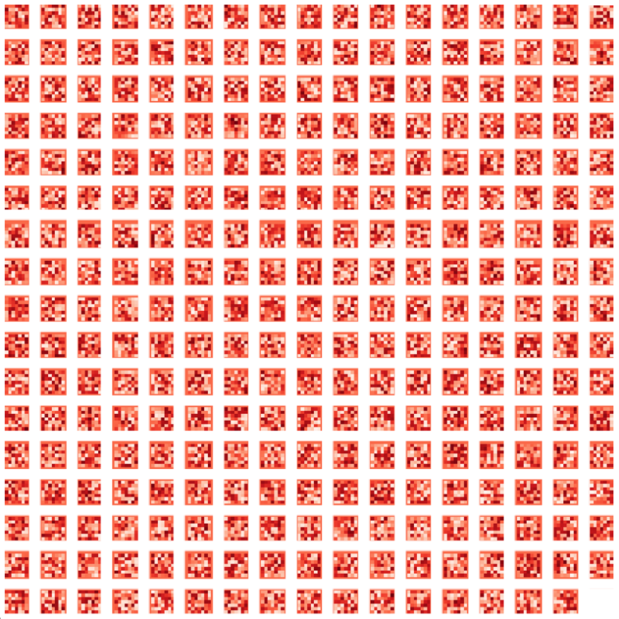
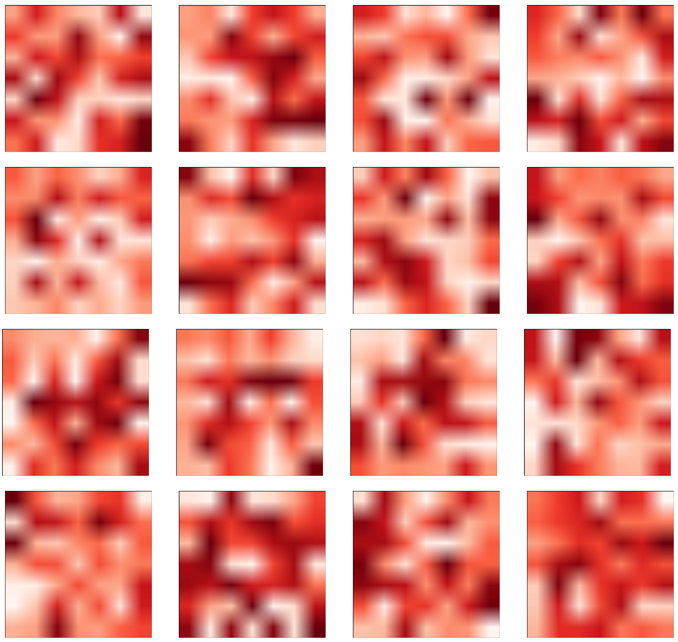
In
Figure 3 and
Figure 4 we illustrate how the filters of the first convolutional layer were shaped after the learning process. Feature extraction is then based on the final weight values of those filters. Darker regions correspond to the most important learned weights while brighter ones have a lower impact on the convolution outcome.
To highlight the superiority of the proposed CNN architecture against other deep-learning-based approaches we conducted two additional experiments where we compare our method against current state-of-the-art methods.
In
Table 4 we show how CNN_EM compares against the work in [
26] when RAW spectrograms are used
without performing semi-supervised feature selection or any other kind of post or pre-possessing. As in [
26] we performed 3 different experimental setups.
Single-Speaker: where training and testing sets correspond to a single speaker
Speaker-Dependent: where samples from multiple speakers are used for training and testing takes place on different samples which belong to the same set of speakers
Speaker-Independent: where samples from multiple speakers are used for training and testing takes place on samples which belong to a different set of speakers
We evaluate on the two datasets that are common ground between the two works, namely the Savee and German (Emo-DB as referenced in [
26]). For comparison purposes we evaluate our method on the original versions of the respective datasets, i.e., without data augmentation. As the results indicate, CNN_EM significantly outperforms their approach in all cases when RAW spectrograms are used as an input to the structure.
In
Table 5 we compare CNN_EM’s scores against the results reported in [
30], on the IEMOCAP Database [
44]. We evaluated CNN_EM on the same set of target classes as in [
30] (
excitement,
happiness,
frustration,
neutral and
surprise) and by splitting the data into training and testing sets in a 80% to 20% ratio per class respectively, as reported in their work. CNN_EM outperforms their best results by 2% without any kind of additional pre-processing in contrast to [
30].
7. Discussion and Conclusions
Multidomain Speech Emotion recognition is a technology that has attracted the interest of numerous applications and satellite sciences of Computer Science. Video and audio stream retrieval for brand monitoring purposes, cognitive sciences for rehabilitation purposes, group dynamics analysis, HRI and HCI related, intelligent interfaces are only few of the domains that such systems are already or have great potential to be deployed. In this work we present an approach that does not require any low-level features. Instead, it uses a Convolutional Neural Network, trained using raw speech information encoded as a spectrogram image. We compare the proposed approach using cross-language datasets and demonstrate that it is able to provide superior results vs. traditional ones that use either audio-based or image-based hand-crafted features.
We show that modern deep learning approaches and especially CNNs, which have been traditionally used for image retrieval related problems, have the potential to produce breakthrough results in cross-modality problems. Language-Independent emotion recognition is a very highly complex problem even for humans. After extensive experimentation, we propose a new CNN architecture, CNN_Emotion, for the the task of Multidomain Speech Emotion Recognition and we show that deep CNN structures have the potential to further outperform current state-of-the-art, even when the data availability is relatively limited.
Our future goals are focused towards two major directions. Firstly we would like to increase the robustness of the proposed method in the given dataset, by further optimising the learning process of the CNN. We believe, that additional research on the initial audio segmentation signal along with the implementation of an enhanced learning technique (i.e., hand-crafted and deep feature fusion) could lead to further improvements. Lastly, our goal is to increase the size of our dataset by adding extra language variations under the rules of a taxonomy. Our assumption is that cultural language similarities could potentially give rise to extra features that were too difficult to be distinguished with the current approach.


 and
and 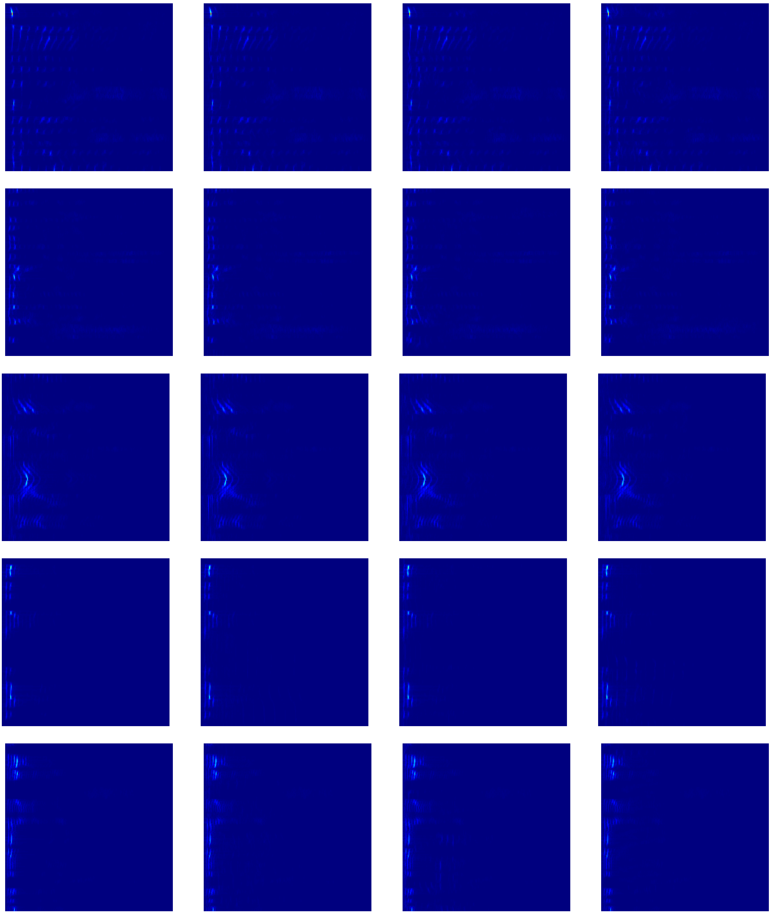
