A Non-Isothermal Chemical Lattice Boltzmann Model Incorporating Thermal Reaction Kinetics and Enthalpy Changes


Earth Life Science Institute, Tokyo Institute of Technology, Tokyo 152-8550, Japan; [email protected]; Tel.: 81-3-5734-2740
†
Current address: 2-12-1-I7E-323, Ookayama, Meguro, Tokyo 152-8550, Japan
Computation 2017, 5(3), 37; https://doi.org/10.3390/computation5030037
Submission received: 31 May 2017
/
Revised: 5 August 2017
/
Accepted: 7 August 2017
/
Published: 9 August 2017
(This article belongs to the Special Issue CFD: Recent Advances in Lattice Boltzmann Methods)
Abstract
:The lattice Boltzmann method is an efficient computational fluid dynamics technique that can accurately model a broad range of complex systems. As well as single-phase fluids, it can simulate thermohydrodynamic systems and passive scalar advection. In recent years, it also gained attention as a means of simulating chemical phenomena, as interest in self-organization processes increased. This paper will present a widely-used and versatile lattice Boltzmann model that can simultaneously incorporate fluid dynamics, heat transfer, buoyancy-driven convection, passive scalar advection, chemical reactions and enthalpy changes. All of these effects interact in a physically accurate framework that is simple to code and readily parallelizable. As well as a complete description of the model equations, several example systems will be presented in order to demonstrate the accuracy and versatility of the method. New simulations, which analyzed the effect of a reversible reaction on the transport properties of a convecting fluid, will also be described in detail. This extra chemical degree of freedom was utilized by the system to augment its net heat flux. The numerical method outlined in this paper can be readily deployed for a vast range of complex flow problems, spanning a variety of scientific disciplines.
1. Introduction
The lattice Boltzmann method (LBM) is a kinetic-based computational fluid dynamics (CFD) technique that was traditionally viewed as a somewhat esoteric, alternative paradigm for the simulation of hydrodynamic systems. It originated from the lattice gas cellular automata (LGCA) [1,2,3], which is a discrete fluid model involving the movement and collision of particles on a lattice. The LGCA attracted interest because it was based on a fictitious mode of molecular interactions, but was nonetheless shown to reproduce the standard Navier–Stokes equations. However, due to its particulate nature, it suffered from considerable stochastic noise and required coarse-graining and other modifications to be mapped onto many systems of interest. It remains useful for exploring concepts of statistical mechanics and dynamical systems theory [4,5], but is less popular for conventional CFD problems.
When the LGCA is coarse-grained, the propagation and collision of individual particles become the propagation and modification of probability distribution functions for a discrete set of particle velocities [2,3]. Fluid mass is encoded in these velocity distribution functions, which move under their own characteristic velocity vectors and exchange mass at discrete grid points due to inter-particle collisions [6,7,8,9,10]. Thus, the LBM is a kinetic-based model, which does not solve the equations of motion for a fluid in the continuum limit, but instead solves for the evolution of velocity distribution functions. With a discrete set of velocities and a suitably-discretized spatial and time domain, the LBM can accurately model a range of flow systems, and a suitable multi-scale analysis can be used to derive the Navier–Stokes equations from the governing equations of the LBM [10,11].
Given its kinetic nature, the LBM can also be expanded to include the advection and diffusion of internal energy [12,13,14,15,16,17,18], alongside the advection and diffusion of momentum. Heat is included as a passively advected scalar quantity, with an extra set of distribution functions. By extension of this logic, further passive scalars can be added. This allows multi-phase and multi-component fluids to be simulated [19,20,21,22]. Versions in recent years have developed yet further and incorporated a range of interactions between these additional components, advancing the LBM into the realm of chemistry [23,24,25,26,27], including thermal chemical problems such as combustion [28,29,30,31].
There are two objectives of the present work: (1) to provide a pedagogical mini review of a general LBM framework that has become a commonly-deployed model for thermal and chemical flow systems; (2) to present new results from an investigation of the transport properties of a convective, reacting fluid system. The key features and equations of the numerical method will be described, and several example systems will be presented for the purpose of validating the method’s efficacy.
The first sections will present the single-phase LBM, followed by the two-population thermal version, and example applications will be discussed. The introduction of additional components and chemical reactions will then be described. A simple, analytically-tractable decay reaction will be simulated, and it will be shown that the reactive LBM (RLBM) is second order accurate, in line with its single-phase counterpart. A simple method for extending the RLBM to include thermal reaction rates and enthalpy changes will then be outlined. The penultimate section explores a system that addresses a simple question in the field of transport phenomena: to what extent can the presence of chemical species and reactions alter the heat flux dynamics of a convecting fluid? The paper concludes with a brief discussion, and suggestions are given for the many applications to which this form of LBM could be amenable.
2. Chemical Lattice Boltzmann Algorithm
2.1. Single-Phase Fluid
For simulating the hydrodynamics of single-phase fluids, the most basic LBM is a relatively simple CFD method. As a kinetic-based scheme, it can either be thought of as deriving directly from the non-equilibrium Boltzmann equation:
or as the result of a coarse-grained averaging of the LGCA [1,2,3]. Equation (1) describes changes in the velocity distribution function as a result of self-advection and particle collisions (represented by the function ). The expression above can be recast into a system with a finite set of discrete velocities (e.g., the D2Q9 system in two dimensions, see below), which can then be discretized in space and time. The exact discretisation method depends on the type of LBM being used (see, e.g., Dellar [32]); in this work, a hidden, semi-implicit scheme is employed.
Assuming a simplification of the collision term in the above equation, wherein the velocity distribution functions relax towards their respective equilibria (given by a suitable discretization of the Boltzmann distribution) at a single characteristic rate , we arrive at the governing equation for the LBM [3,7,10,16,33]:
where i indexes the discrete velocity set, is the velocity distribution for velocity i (a measure of the fluid mass possessing velocity i at that point in space and time), is the velocity vector, is the time step, is the relaxation time scale and is the equilibrium distribution:
where is the lattice weight for velocity i, is the lattice speed and is the speed of sound. The use of a single-time relaxation step is commonly known as the lattice Bhatnagar, Gross and Krook (LBGK) method [34].
Fluid properties are calculated from the appropriate moments of the distribution function, including density and velocity (higher order moments can also be used to calculate internal energy density and viscous stresses, etc.),
All modeling in the present work is carried out using the two-dimensional D2Q9 velocity set, which utilizes a square lattice with eight velocities and rest particles. For this set, the velocity weights are , for and for . The velocity vectors are thus:
Using the Chapman–Enskog expansion, it can be shown that at the macro-level, a fluid obeying the above equations satisfies the Navier–Stokes equations (see, e.g., Chen and Doolen [7], Succi [10]) with a kinematic viscosity given by
Many years of analysis have revealed that the above-described model can reproduce incompressible flow dynamics to second order accuracy [6,7,8,9,10,35]. Furthermore, the LBM can be applied to turbulent flows [6,10,36], and recent novel lattice schemes [37], entropic multi-speed approaches [38] and cumulant methods [39] have further broadened the range of applications amenable to simulation by the LBM.
2.2. Thermohydrodynamics
As the LBM developed further, researchers began probing its ability to simulate thermohydrodynamic, multi-phase and multi-component systems. What emerged were two main methods for simulating the internal energy density of a modeled fluid. Given the intrinsic connection between local temperature and particle velocities, one can derive the temperature from the appropriate moment of the velocity distribution function [14,16,40]:
where D is the spatial dimension, R is the molar gas constant, is the distribution function before discretisation, is the particle velocity, is the net fluid velocity and is the distribution function for internal energy density. The integral is taken over the entire (continuous) velocity space.
After discretisation, this integral becomes:
It is possible to construct simulations in which only the evolution of the velocity distribution function needs to be modeled. However, one must include more than one characteristic relaxation time and the method suffered from various issues including instability and the presence of spurious physical effects [41,42,43]. Note that this approach was more recently developed into a fully-consistent method using the entropic lattice Boltzmann approach [13].
The alternative to multi-speed models is to track the internal energy distribution using an additional set of distribution functions. He et al. [14] developed a thermal LBM wherein the function is discretized in velocity space, physical space and time in the same way that is discretized in the standard LBM. This method was then simplified by Peng et al. [18] into the following form.
The discretized internal energy distribution function evolves analogously to the velocity distribution function:
where is the characteristic relaxation time for internal energy. This parameter controls the thermal diffusivity:
The equilibrium distribution functions for the internal energy in the D2Q9 velocity system are given by [18]:
Many thermohydrodynamic problems are related to natural convection, in which buoyancy forces produce fluid accelerations due to temperature (and hence density) differences. Such an effect can easily be incorporated into the LBM framework using the Boussinesq approximation, in which it is assumed that density differences are negligible except with regard to the generation of buoyancy forces. The body force is represented by an additional term in the evolution equation for the velocity distribution function, which subsequently becomes:
The body force term is given by:
where is the mean temperature, is the vector representing the buoyancy force, is the thermal expansion coefficient and is gravitational acceleration [14,18]. As with the single-phase system, this model has been validated over many years by repeated analyses and comparisons with analytical and experimental results [14,16,18,44,45]. It has been successfully applied to a variety of thermal flow problems including natural convection [14,18,44,46,47,48,49,50], turbulent convection [51,52,53,54], thermal channel flows [14,40,55,56] and more complex systems involving multiple phases and phase change [57,58,59,60,61,62,63,64,65].
There have also been efforts to understand the relationship between natural convection and the principle of maximum entropy production (MEP) [66,67,68] (see Dyke and Kleidon [69], Martyushev and Seleznev [70] and references therein for details of the MEP principle). It was found that while previous authors proposed that natural convection was a prime example of MEP [71,72], in fact, this is not the case. The MEP prediction does not take proper account of the physical properties of the system in question (hence its generality), but convective heat flux is a strong function of the parameters of the system and is far more constrained than atmospheric flows (in which MEP predictions can be quite accurate [73,74,75]). A variety of counter examples, generated using LBM simulations, showed that MEP does not in fact predict the steady states of a convective fluid [66,67,76].
2.3. Dissolved Chemical Species
As well as internal energy, the LBM can readily include further additional components (see, e.g., [19,21]) (note that the original work in this direction was carried out by Gunstensen et al. [20]). There are a variety of approaches to this problem of multi-component fluids [22,23,25,29,30,77,78,79], but arguably the simplest and most commonly-used involves a simple addition of distribution functions corresponding to each extra component in the fluid. The physical assumption underlying this approach is that the additional components are low in concentration such that they do not explicitly influence the fluid flow. They are classed as passive scalars and are advected by any net fluid velocity. Under this assumption, any number of extra species can be added, and they follow analogous evolution equations to the internal energy:
where is the component index and is the relaxation time. The equilibrium distributions take on the following form:
where represents the concentration of species . Note that unlike Equation (3), higher order terms can be neglected from these distributions, since they were shown to be unnecessary by Ayodele et al. [24] (assuming the Mach number is kept low). Those authors found that both the linear and quadratic forms of the equilibrium distributions were second order accurate. The diffusivity of species is given by:
and the concentration by:
2.4. Isothermal Reactive LBM
The RLBM described above requires further modifications to allow interactions between the components. The simplest way to introduce chemical reactions is to add extra terms to Equation (15). It will be assumed that the chemical kinetics can be described using a standard mass action rate law.
2.4.1. Single Reaction Benchmark Test
As an example test case, the irreversible decay of a reactant in a closed system with no fluid motion is particularly favorable. Such a system can be described by a pair of coupled differential equations:
which can be solved analytically using Fourier transforms. This yields an expression for the concentration field of species A:
where it has been assumed that the mass of species A is initially concentrated at the point , thus . Note that is the Thiele modulus, a dimensionless parameter that measures the ratio of the characteristic reaction time to that of mass diffusion. For systems that are very large, have a high rate constant or a low mass diffusivity, , and the reaction will be the dominant process. If , because of a combination of small characteristic length, low reaction rate and/or high diffusivity, the dynamics of the system are dominated by the process of diffusion, and reaction plays only a minor role. In this work, .
It is straightforward to construct the RLBM equations for modeling this system. The two passive scalar species are governed by the following equations:
where k is the rate constant. The equilibria for this system are simplified due to the lack of fluid motion and everywhere):
The RLBM results can now be compared to the exact solution of Equation (21), as was done by Ayodele et al. [23]. The present assessment differs slightly in that all simulations were initialized at dimensionless time and run through to . This was motivated by the desire to avoid initial conditions with large discontinuities. Such discontinuities are inevitable if the simulation is initiated simply with unit concentration of the reactant at the central grid node, i.e., when . The numerical error is calculated using:
and is plotted for a range of relaxation parameters and rate constants k in Figure 1.
Note that in order to compare the same problem for different parameter combinations, the dimensionless group and the dimensionless end time t must be kept constant. Thus, the characteristic length L (grid size) was appropriately adjusted for each pair.
As one might expect, smaller reaction rates and larger diffusivities produce lower errors. The errors are very similar in magnitude to those found by Ayodele et al. [23]; however, there are no minima in the error curves here. Using a third-order Chapman–Enskog expansion, Ayodele et al. [23] derived an expression for E as a function of various system parameters and found crucially that it is a quadratic function of the relaxation parameter , but also contains several derivatives of the density . They concluded that since their error curves were not parabolic, errors were clearly entering into the system due to derivatives of the density. The different shapes of the curves in Figure 1 compared to those of Ayodele et al. [23] are probably related to the different initial conditions used in the present work. However, in agreement with Ayodele et al. [23], it was found that there is a linear dependence between the error and the rate constant k.
In conclusion, it is clear that the RLBM is capable of simulating simple reactive systems. The appropriate Chapman–Enskog expansions have been shown to recover the relevant reaction-diffusion equations, and the method is second order accurate, in line with the single-phase version [23,77]. Variants of this RLBM have been used to model a range of chemical flow systems including the velocity and chemical species distribution around a reacting block in a channel flow [80], reactive dissolution and precipitation of solid and porous materials [81,82,83,84], as well as heterogeneous catalysis in microflows [85,86].
2.4.2. Pattern Formation in the Gray–Scott System
This section will present a more detailed application of the RLBM to a non-linear, pattern-forming chemical system known as the Gray–Scott reaction diffusion system (GSRDS) [87,88,89]. Its defining characteristic is an autocatalytic reaction that allows stable or oscillatory structures to form in the concentration fields of the chemical species. As the two main parameters of the system are varied, a vast suite of different patterns is exhibited, including plane waves, spiral waves, lamellar phases and circular solitons, or spots [76,88,89,90,91,92,93]. Such a characteristic example of non-equilibrium pattern formation is a prime candidate for testing hypotheses regarding the thermodynamics of dissipative structures and the relationship of such structures to the self-organization processes that contributed to the origin of life [94,95]. Understanding such self-organization processes could also guide future work in the fields of microfluidics and nanotechnology [96].
The majority of past investigations of the GSRDS were analytical or numerical, due to its interesting mathematical properties as a non-linear dynamical system, capable of exhibiting spatio-temporal chaos and complex pattern formation. These features made it an ideal exemplar of the original ideas of Turing [97]. Despite the simplicity of the GSRDS, experimental work has shown that it can be readily mapped to the ferrocyanide-iodate-sulfite reaction, which exhibits a similar range of oscillatory and pattern-forming behaviors [90,98,99].
The GSRDS is described by the following equations:
where the second RHS terms represent the autocatalytic reaction and the third terms implement porous wall BCs. These BCs act to maintain the concentration of species A close to unity and the concentration of species B close to zero. The strength of these supply and removal terms is controlled by the two parameters F and R. Note that the pattern formation process relies upon the following diffusivity constraint: . One can vary F and R freely and observe the aforementioned range of stable and dynamic structures.
In the case of non-zero solvent velocity, the two equations above gain an extra advection term and become:
The dynamics of the GSRDS can be reproduced by the RLBM with the following evolution equations:
with equilibria defined by Equation (16). Such an RLBM system was explored for a still fluid by Ayodele et al. [23], under several parameter combinations, and subsequently for a sheared fluid [24].
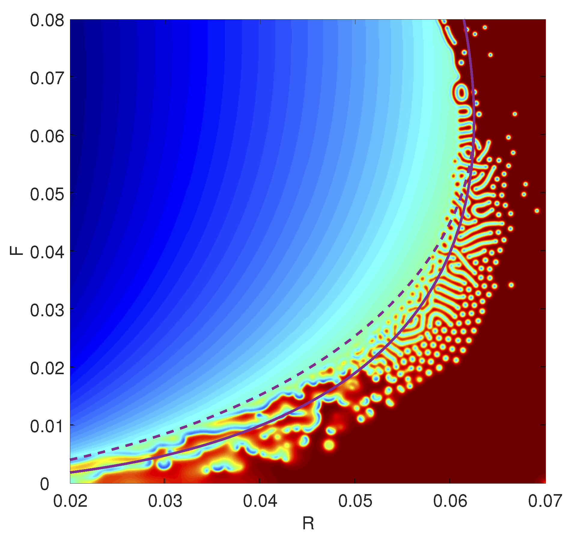
As a comprehensive assessment of the RLBM’s ability in the context of the GSRDS, the entire phase space of chemical patterns can be reproduced by simulating a system in which the two parameters F and R vary as a function of the vertical and horizontal coordinate, respectively. An instantaneous snapshot from such a system is shown in Figure 2.
This phase diagram agrees well with analogous diagrams in previous works [89,91] and highlights the complex emergent properties of this simple system. As was found by Ayodele et al. [23], the characteristic size of the chemical structures can be modified by changing the diffusivity (keeping the ratio constant). This is achieved in the RLBM simply by changing the relaxation parameters and . To highlight this effect, Figure 3 shows four different phase portraits, each with a different value of .
These phase diagrams highlight the coarse-graining effect of increasing the diffusivities of the two species, which affects all patterns in an essentially equivalent manner. Thus, we now see how the three key parameters of the system can be tuned to produce any desired pattern from the system’s repertoire. Changes in F and R take the system through different structural phases, and changes in allow a simple increase or decrease of the characteristic pattern length scale.
Such observations can be leveraged for the exploration of more complex interactions in systems with large numbers of interacting chemical species. If there were mutual catalytic enhancements and inhibitions, as well as physical interactions such as modulations of viscosity and/or passive scalar diffusivities, one can imagine a vast range of potential life-like dynamics, including competition, symbiosis and arms races.
2.5. Thermal Reactive LBM
The isothermal constraint of the RLBM is somewhat limiting. A vast range of important systems involves the coupled dynamics of reactions, heat transfer and convection (e.g., Andres and Cardoso [100], Rogers and Morris [101]). One of the most common applications of thermal RLBMs (TRLBMs) has been for problems of combustion [28,29,30,77,78,79]. This section will present a simple approach to relaxing the isothermal assumption of the RLBM, beginning with thermal rate constants and moving on to enthalpy changes.
Chemical reaction rates are functions of many variables (pressure, cross-section of reactant molecules, etc.), but one of the most influential is temperature. The temperature dependence of simple reactions is encapsulated in the Arrhenius equation, which expresses the rate in terms of the frequency factor A, activation energy E and temperature T:
which can simply replace the constant rate parameter used to scale reactions in the isothermal RLBM.
Another crucial thermal feature of reactions is changes in enthalpy from the reactant to product state. If we assume that no pressure-volume work is done during a reaction, any free energy difference will be released as a local change in internal energy, i.e., a gain or loss of heat. In the majority of LBMs, the fluid is assumed to be incompressible, which automatically constrains the model to cases of negligible compression work from reactions. If we follow the standard convention of a negative enthalpy change implying an exothermic reaction, the internal energy distributions of a TRLBM are governed by:
where R is the number of reactions, , and are the frequency factor, activation energy and enthalpy change of reaction k, N is the number of chemical species and is the stoichiometric coefficient for reaction k and chemical species l.
In addition to combustion, variants of the TRLBM have been applied to several complex fluid problems including microfluidics [102] and fuel cells [103]. It has also been used to explore thermal effects in the GSRDS. The addition of thermal rate constants and finite reaction enthalpies introduced a completely new set of physical effects. A strongly endothermic reaction in a convecting fluid produced a competitive dynamic, in which chemical structures and convection plumes were observed to compete for a common heat source. This behavior was analogous to ecological effects, allowing compelling parallels to be drawn between non-living dissipative structures and organisms [76,104].
It was also found that two sets of GSRDSs embedded in the same system could exhibit spontaneous temperature regulation, if one set had an exothermic reaction and the other an endothermic reaction. The composite system was found to be robust to large changes of boundary temperature, even when such changes would normally eliminate the conditions for stable pattern formation [105]. This was a further example of an effect strongly reminiscent of the living world (homeostasis), exhibited by a purely physicochemical system.
2.5.1. Reversibility and Heat Transport Enhancement
This final section will present new results from a study in which the TRLBM was used to address a simple thermodynamic transport problem. The system in question will be a two-dimensional fluid with two solute species undergoing a reversible reaction . If a steady vertical temperature gradient is imposed on the system, it will respond with a net heat flux in the same direction. This heat flux is normally constrained by the physical properties of the fluid (viscosity, thermal diffusivity and coefficient of thermal expansion) and buoyancy force (strength of gravity), as well as the strength of the temperature gradient. If that gradient is strong enough, the fluid will undergo convective motion. With the two chemical species and reaction present, the net heat flux of the system will be affected (assuming non-zero enthalpy change ). We can ask whether it will be enhanced or diminished, and if so, how does this scale with the amount of chemical species present. They represent an extra degree of freedom that the system can potentially make use of.
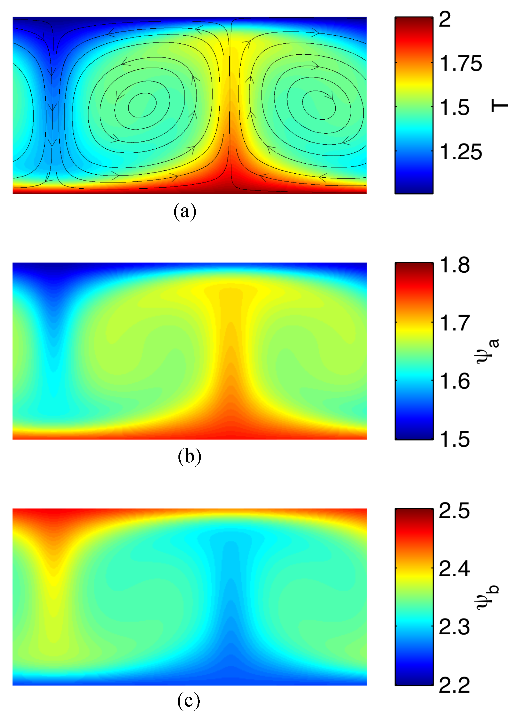
To address this problem, a series of simulations of a single size were carried out, with two different sets of fluid parameters. The first set had a Rayleigh number of , and the second had a value of . For each of the two Rayleigh numbers, simulations were performed with fixed temperature BCs, and also with fixed flux BCs. The total mass of chemical species present in the system was varied for each run (but held constant during the run, there was no flux of mass in or out of the system). It was raised from zero to a value that gave mean concentrations of . Each simulation was initialized with a small amount of noise and concluded when a steady state was reached. Figure 4 displays the steady state configuration of a simulation with , fixed temperature BCs, and a mean initial chemical species concentration of .
The system configured itself such that the endothermic reverse reaction was more prevalent at the lower, hotter end of the domain, leading to a higher steady state concentration in that region. The forward, exothermic reaction dominated at the cooler upper boundary, yielding higher concentrations of B near the top wall. Indeed, it appears that the system maximized its heat flux by arranging in this way. Having the endothermic reaction dominate at the lower wall means that the system invests heat energy in converting B to A; this energy is carried by A as it is advected by the flow before being released gradually as the reaction changes to at the upper wall. The two chemical species and their reaction have been utilized as an additional heat delivery mechanism in parallel with the advection and diffusion of heat alone. Note, however, that the velocity field is identical to that of a purely convective, Rayleigh–Bénard system (see Figure 4a).
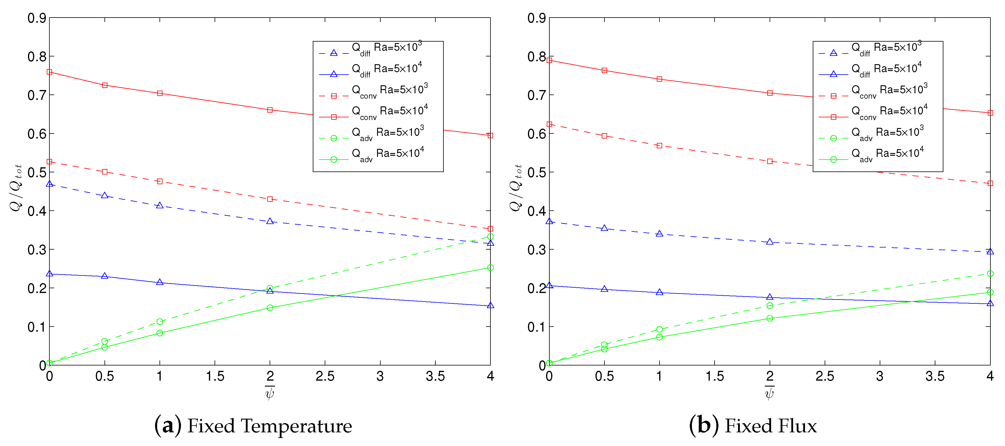
It is straightforward to quantify the heat transport increase exhibited by these systems. Figure 5 shows the different components of heat flux as a function of average chemical species concentration. The heat flux values are normalized by total heat flux; thus, the curves show fractional contributions to the three different modes of heat transport: diffusion, convection and advection by chemical species. Similar trends can be seen for both types of BC. With increases in chemical species concentration, an increasing heat transport function is exhibited by the chemical aspect of the system, and the relative roles of the other heat transport mechanisms are reduced. It seems the system is gradually switching over to a configuration in which advection and reaction provide an increasingly larger fraction of the total heat transport. This makes sense because higher quantities of chemical species mean that the heat exchange as a result of reactions will increase, and the amount of heat that can be invested in the enthalpy of chemical species also increases.
However, one would expect that this trend cannot continue ad infinitum. There is likely to be a lower limit for the diffusive heat transport (in the fixed boundary temperature case, the absolute diffusive heat flux is constant since the temperature difference and thermal diffusivity are constant), since all heat must enter and leave the system by diffusion. The blue curves of Figure 5 appear to have a decreasing curvature with a gradient that seems to be tending to zero.
Considering the role of convection, it should be kept in mind that the advection of chemical species relies on there being a sustained fluid flow. That fluid flow is induced by the temperature gradient, and so, in the case of fixed flux BCs, as the system becomes ”more efficient” at transporting heat, it gradually diminishes the driving force for the generation of buoyant motion. Thus, for these BCs, it is likely that there will be an eventual saturation of the relative magnitude of chemical advective heat transport.
In the fixed temperature case, this can never be an issue because the driving force is constant (the boundary heat flux adjusts itself to maintain the boundary temperatures at their relevant values). One observation that is not shown in Figure 5 is that for this BC, the total heat flux increased with . The presence of the chemical species enhanced the system’s heat transport abilities, and it used those new abilities to augment its total heat flux above that which would occur without the action of the chemistry.
3. Conclusions
This paper described a powerful version of the LBM, in which fluid dynamics, heat transfer, buoyancy-driven convection, passive scalar advection, chemical reactions and enthalpy changes can all be incorporated simultaneously. The method is a natural extension of previous versions, and it retains the second order accuracy of the standard LBM. It is simple to code and easily parallelizable.
The single-phase and thermohydrodynamic forms of the model were described, and previous applications to natural convection and the validity of the principle of MEP were presented. It was shown that isothermal chemical reactions can be accurately simulated, and the complex, pattern-forming behavior of the GSRDS was comprehensively reproduced. Thermally-resolved systems were then explored, by introducing a temperature-dependent rate factor and reaction-induced internal energy changes due to enthalpy differences. Previous results including ecological phenomena (competition and temperature regulation) of dissipative structures in the thermal GSRDS were discussed.
Finally, an investigation of heat flux enhancement by the reaction and advection of chemical species was presented. It was observed that convecting fluid systems with a reversible reaction between solute species are able to transport more heat than their non-chemical counterparts. The presence of the chemical species provided a parallel channel for heat flow, the spatial structure of which was optimized by the system to maximize total heat flux.
There is an almost limitless range of systems that can be investigated using this TRLBM, since the number of chemical species and reactions can be increased until computational power becomes a binding constraint. Porous media can also be incorporated as they are in the standard LBM, and geochemical systems such as hydrothermal vents can be readily modeled. A range of fields from biophysics to astrobiology to chemical engineering could make use of this method.
4. Further Work
To further validate the present method, it would be useful to take a range of complex thermal chemical systems and compare their results with those of mainstream commercial multi-physics solvers, and perhaps also with laboratory experiments. It would be interesting to explore the limits at which the TRLBM begins to lose accuracy, and the computational efficiency of the method should be compared to more conventional CFD models. Accuracy limits might also be amenable to analytical calculation.
Acknowledgments
This work was supported by an EPSRC Doctoral Training Centre grant (EP/G03690X/1) and the Earth Life Science Institute Origins Network (EON) Postdoctoral Fellowship Program.
Author Contributions
S.B. conceived of the new numerical experiments in this work, wrote and carried out all simulations, produced the figures and wrote the text.
Conflicts of Interest
The author declares no conflict of interest.
Abbreviations
The following abbreviations are used in this manuscript:
| LBM | Lattice Boltzmann method |
| LGCA | Lattice gas cellular automata |
| CFD | Computational fluid dynamics |
| MEP | Maximum entropy production |
| RLBM | Reactive lattice Boltzmann method |
| TRLBM | Thermal reactive lattice Boltzmann method |
| GSRDS | Gray–Scott reaction diffusion system |
| BC | Boundary condition |
References
- Frisch, U.; Hasslacher, B.; Pomeau, Y. Lattice-gas automata for the navier-stokes equation. Phys. Rev. Lett. 1986, 56, 1505–1508. [Google Scholar] [CrossRef] [PubMed]
- McNamara, G.R.; Zanetti, G. Use of the boltzmann equation to simulate lattice-gas automata. Phys. Rev. Lett. 1988, 61, 2332–2335. [Google Scholar] [CrossRef] [PubMed]
- Qian, Y.H.; D’Humières, D.; Lallemand, P. Lattice bgk models for navier-stokes equation. EPL (Europhys. Lett.) 1992, 17, 479. [Google Scholar] [CrossRef]
- Bagnoli, F.; Rechtman, R. Thermodynamic entropy and chaos in a discrete hydrodynamical system. Phys. Rev. E 2009, 79. [Google Scholar] [CrossRef] [PubMed]
- Boghosian, B.M. Lattice gases and cellular automata. Future Gener. Comput. Syst. 1999, 16, 171–185. [Google Scholar] [CrossRef]
- Aidun, C.K.; Clausen, J.R. Lattice-Boltzmann method for complex flows. Annu. Rev. Fluid Mech. 2010, 42, 439–472. [Google Scholar] [CrossRef]
- Chen, S.; Doolen, G.D. Lattice Boltzmann Method for Fluid Flows. Annu. Rev. Fluid Mech. 1998, 30, 329–364. [Google Scholar] [CrossRef]
- D’Humières, D. Multiple–relaxation–time lattice Boltzmann models in three dimensions. Philos. Trans. R. Soc. Lond. A Math. Phys. Eng. Sci. 2002, 360, 437–451. [Google Scholar] [CrossRef] [PubMed]
- Luo, L.S.; Krafczyk, M.; Shyy, W. Lattice Boltzmann Method for Computational Fluid Dynamics. In Encyclopedia of Aerospace Engineering; John Wiley & Sons, Ltd.: Hoboken, NJ, USA, 2010. [Google Scholar]
- Succi, S. The Lattice Boltzmann Equation: For Fluid Dynamics and Beyond; Numerical Mathematics and Scientific Computation, Clarendon Press: Wotton-under-Edge, Glos, UK, 2001. [Google Scholar]
- Sofonea, V.; Sekerka, R.F. Viscosity of finite difference lattice Boltzmann models. J. Comput. Phys. 2003, 184, 422–434. [Google Scholar] [CrossRef]
- Dorschner, B.; Frapolli, N.; Chikatamarla, S.S.; Karlin, I.V. Grid refinement for entropic lattice Boltzmann models. Phys. Rev. E 2016, 94, 053311. [Google Scholar] [CrossRef] [PubMed]
- Frapolli, N.; Chikatamarla, S.S.; Karlin, I.V. Multispeed entropic lattice Boltzmann model for thermal flows. Phys. Rev. E 2014, 90, 043306. [Google Scholar] [CrossRef] [PubMed]
- He, X.; Chen, S.; Doolen, G.D. A Novel Thermal Model for the Lattice Boltzmann Method in Incompressible Limit. J. Comput. Phys. 1998, 146, 282–300. [Google Scholar] [CrossRef]
- Karlin, I.V.; Sichau, D.; Chikatamarla, S.S. Consistent two-population lattice Boltzmann model for thermal flows. Phys. Rev. E 2013, 88, 063310. [Google Scholar] [CrossRef] [PubMed]
- Liu, C.H.; Lin, K.H.; Mai, H.C.; Lin, C.A. Thermal boundary conditions for thermal lattice Boltzmann simulations. Comput. Math. Appl. 2010, 59, 2178–2193. [Google Scholar] [CrossRef]
- Pareschi, G.; Frapolli, N.; Chikatamarla, S.S.; Karlin, I.V. Conjugate heat transfer with the entropic lattice Boltzmann method. Phys. Rev. E 2016, 94, 013305. [Google Scholar] [CrossRef] [PubMed]
- Peng, Y.; Shu, C.; Chew, Y.T. Simplified thermal lattice Boltzmann model for incompressible thermal flows. Phys. Rev. E 2003, 68, 026701. [Google Scholar] [CrossRef] [PubMed]
- Arcidiacono, S.; Karlin, I.; Mantzaras, J.; Frouzakis, C. Lattice Boltzmann model for the simulation of multicomponent mixtures. Phys. Rev. E 2007, 76, 046703. [Google Scholar] [CrossRef] [PubMed]
- Gunstensen, A.; Rothman, D.; Zaleski, S. Lattice Boltzmann model of immiscible fluids. Phys. Rev. A 1991, 43, 4320–4327. [Google Scholar] [CrossRef] [PubMed]
- Luo, L.S.; Girimaji, S. Lattice Boltzmann model for binary mixtures. Phys. Rev. E 2002, 66, 035301. [Google Scholar] [CrossRef] [PubMed]
- Stiebler, M.; Tölke, J.; Krafczyk, M. Advection-diffusion lattice Boltzmann scheme for hierarchical grids. Comput. Math. Appl. 2008, 55, 1576–1584. [Google Scholar] [CrossRef]
- Ayodele, S.G.; Varnik, F.; Raabe, D. Lattice Boltzmann study of pattern formation in reaction-diffusion systems. Phys. Rev. E 2011, 83, 016702. [Google Scholar] [CrossRef] [PubMed]
- Ayodele, S.G.; Raabe, D.; Varnik, F. Lattice Boltzmann modeling of advection-diffusion-reaction equations: Pattern formation under uniform differential advection. Commun. Comput. Phys. 2013, 13, 741–756. [Google Scholar] [CrossRef]
- Dawson, S.; Chen, S.; Doolen, G.D. Lattice Boltzmann computations for reaction-diffusion equations. J. Chem. Phys. 1993, 98, 1514–1523. [Google Scholar] [CrossRef]
- Kang, J.; Prasianakis, N.I.; Mantzaras, J. Thermal multicomponent lattice Boltzmann model for catalytic reactive flows. Phys. Rev. E 2014, 89, 063310. [Google Scholar] [CrossRef] [PubMed]
- Zhang, J.; Yan, G. Lattice Boltzmann model for the bimolecular autocatalytic reaction–diffusion equation. Appl. Math. Model. 2014, 38, 5796–5810. [Google Scholar] [CrossRef]
- Chen, S.; Liu, Z.; Tian, Z.; Shi, B.; Zheng, C. A simple lattice Boltzmann scheme for combustion simulation. Comput. Math. Appl. 2008, 55, 1424–1432. [Google Scholar] [CrossRef]
- Chiavazzo, E.; Karlin, I.V.; Gorban, A.N.; Boulouchos, K. Combustion simulation via lattice Boltzmann and reduced chemical kinetics. J. Stat. Mech. Theory Exp. 2009, 2009, P06013. [Google Scholar] [CrossRef]
- Chiavazzo, E.; Karlin, I.V.; Gorban, A.N.; Boulouchos, K. Coupling of the model reduction technique with the lattice Boltzmann method for combustion simulations. Combust. Flame 2010, 157, 1833–1849. [Google Scholar] [CrossRef]
- Yamamoto, K.; He, X.; Doolen, G.D. Simulation of Combustion Field with Lattice Boltzmann Method. J. Stat. Phys. 2002, 107, 367–383. [Google Scholar] [CrossRef]
- Dellar, P.J. An interpretation and derivation of the lattice Boltzmann method using Strang splitting. Comput. Math. Appl. 2013, 65, 129–141. [Google Scholar] [CrossRef]
- He, X.; Luo, L.S. Theory of the lattice Boltzmann method: From the Boltzmann equation to the lattice Boltzmann equation. Phys. Rev. E 1997, 56, 6811–6817. [Google Scholar] [CrossRef]
- Bhatnagar, P.L.; Gross, E.P.; Krook, M. A Model for Collision Processes in Gases. I. Small Amplitude Processes in Charged and Neutral One-Component Systems. Phys. Rev. 1954, 94, 511–525. [Google Scholar] [CrossRef]
- Geller, S.; Krafczyk, M.; Tolke, J.; Turek, S.; Hron, J. Benchmark computations based on lattice-Boltzmann, finite element and finite volume methods for laminar flows. Comput. Fluids 2006, 35, 888–897. [Google Scholar] [CrossRef]
- Karlin, I.V.; Bösch, F.; Chikatamarla, S.S. Gibbs’ principle for the lattice-kinetic theory of fluid dynamics. Phys. Rev. E 2014, 90, 031302. [Google Scholar] [CrossRef] [PubMed]
- Frapolli, N.; Chikatamarla, S.S.; Karlin, I.V. Lattice Kinetic Theory in a Comoving Galilean Reference Frame. Phys. Rev. Lett. 2016, 117, 010604. [Google Scholar] [CrossRef] [PubMed]
- Frapolli, N.; Chikatamarla, S.S.; Karlin, I.V. Entropic lattice Boltzmann model for compressible flows. Phys. Rev. E 2015, 92, 061301. [Google Scholar] [CrossRef] [PubMed]
- Geier, M.; Schönherr, M.; Pasquali, A.; Krafczyk, M. The cumulant lattice Boltzmann equation in three dimensions: Theory and validation. Comput. Math. Appl. 2015, 70, 507–547. [Google Scholar] [CrossRef]
- Shi, Y.; Zhao, T.S.; Guo, Z.L. Thermal lattice Bhatnagar-Gross-Krook model for flows with viscous heat dissipation in the incompressible limit. Phys. Rev. E 2004, 70, 066310. [Google Scholar] [CrossRef] [PubMed]
- Chen, Y.; Ohashi, H.; Akiyama, M. Two-Parameter Thermal Lattice BGK Model with a Controllable Prandtl Number. J. Sci. Comput. 1997, 12, 169–185. [Google Scholar] [CrossRef]
- Chen, H.; Teixeira, C. H-theorem and origins of instability in thermal lattice Boltzmann models. Comput. Phys. Commun. 2000, 129, 21–31. [Google Scholar] [CrossRef]
- Teixeira, C.; Chen, H.; Freed, D.M. Multi-speed thermal lattice Boltzmann method stabilization via equilibrium under-relaxation. Comput. Phys. Commun. 2000, 129, 207–226. [Google Scholar] [CrossRef]
- Peng, Y.; Shu, C.; Chew, Y. A 3D incompressible thermal lattice Boltzmann model and its application to simulate natural convection in a cubic cavity. J. Comput. Phys. 2004, 193, 260–274. [Google Scholar] [CrossRef]
- Shan, X. Simulation of Rayleigh-Bénard convection using a lattice Boltzmann method. Phys. Rev. E 1997, 55, 2780–2788. [Google Scholar] [CrossRef]
- D’Orazio, A.; Corcione, M.; Celata, G.P. Application to natural convection enclosed flows of a lattice Boltzmann BGK model coupled with a general purpose thermal boundary condition. Int. J. Therm. Sci. 2004, 43, 575–586. [Google Scholar] [CrossRef]
- Guo, Z.; Zhao, T. Lattice Boltzmann simulation of natural convection with temperature-dependent viscosity in a porous cavity. Prog. Comput. Fluid Dyn. Int. J. 2005, 5, 110–117. [Google Scholar] [CrossRef]
- Kao, P.H.; Yang, R.J. Simulating oscillatory flows in Rayleigh Bénard convection using the lattice Boltzmann method. Int. J. Heat Mass Transf. 2007, 50, 3315–3328. [Google Scholar] [CrossRef]
- Rong, F.; Guo, Z.; Zhang, T.; Shi, B. Numerical study of Bénard convection with temperature-dependent viscosity in a porous cavity via lattice Boltzmann method. Int. J. Mod. Phys. C 2010, 21, 1407–1419. [Google Scholar] [CrossRef]
- Watanabe, T. Flow pattern and heat transfer rate in Rayleigh Bénard convection. Phys. Fluids 2004, 16, 972–978. [Google Scholar] [CrossRef]
- Chen, S.; Krafczyk, M. Entropy generation in turbulent natural convection due to internal heat generation. Int. J. Therm. Sci. 2009, 48, 1978–1987. [Google Scholar] [CrossRef]
- Chen, S.; Tölke, J.; Krafczyk, M. Simple lattice Boltzmann subgrid-scale model for convectional flows with high Rayleigh numbers within an enclosed circular annular cavity. Phys. Rev. E 2009, 80, 026702. [Google Scholar] [CrossRef] [PubMed]
- Dixit, H.; Babu, V. Simulation of high Rayleigh number natural convection in a square cavity using the lattice Boltzmann method. Int. J. Heat Mass Transf. 2006, 49, 727–739. [Google Scholar] [CrossRef]
- Van Treeck, C.; Rank, E.; Krafczyk, M.; Tölke, J.; Nachtwey, B. Extension of a hybrid thermal LBE scheme for large-eddy simulations of turbulent convective flows. Comput. Fluids 2006, 35, 863–871. [Google Scholar] [CrossRef]
- D’Orazio, A.; Succi, S. Simulating two-dimensional thermal channel flows by means of a lattice Boltzmann method with new boundary conditions. Future Gener. Comput. Syst. 2004, 20, 935–944. [Google Scholar] [CrossRef]
- Tian, Z.W.; Zou, C.; Liu, H.; Liu, Z.; Guo, Z.; Zheng, C. Thermal lattice boltzmann model with viscous heat dissipation in the incompressible limit. Int. J. Mod. Phys. C 2006, 17, 1131–1139. [Google Scholar] [CrossRef]
- Chang, Q.; Alexander, J.I.D. Application of the lattice Boltzmann method to two-phase Rayleigh-Bénard convection with a deformable interface. J. Comput. Phys. 2006, 212, 473–489. [Google Scholar] [CrossRef]
- Chen, S.; Tölke, J.; Krafczyk, M. Simulation of buoyancy-driven flows in a vertical cylinder using a simple lattice Boltzmann model. Phys. Rev. E 2009, 79, 016704. [Google Scholar] [CrossRef] [PubMed]
- Huber, C.; Parmigiani, A.; Chopard, B.; Manga, M.; Bachmann, O. Lattice Boltzmann model for melting with natural convection. Int. J. Heat Fluid Flow 2008, 29, 1469–1480. [Google Scholar] [CrossRef]
- Inamuro, T. Lattice Boltzmann methods for viscous fluid flows and for two-phase fluid flows. Fluid Dyn. Res. 2006, 38, 641–659. [Google Scholar] [CrossRef]
- Inamuro, T.; Yoshino, M.; Inoue, H.; Mizuno, R.; Ogino, F. A Lattice Boltzmann Method for a Binary Miscible Fluid Mixture and Its Application to a Heat-Transfer Problem. J. Comput. Phys. 2002, 179, 201–215. [Google Scholar] [CrossRef]
- Safari, H.; Rahimian, M.H.; Krafczyk, M. Extended lattice Boltzmann method for numerical simulation of thermal phase change in two-phase fluid flow. Phys. Rev. E 2013, 88, 013304. [Google Scholar] [CrossRef] [PubMed]
- Safari, H.; Rahimian, M.H.; Krafczyk, M. Consistent simulation of droplet evaporation based on the phase-field multiphase lattice Boltzmann method. Phys. Rev. E 2014, 90, 033305. [Google Scholar] [CrossRef] [PubMed]
- Yuan, P.; Schaefer, L. A thermal lattice Boltzmann two-phase flow model and its application to heat transfer problems part 1. Theoretical foundation. J. Fluids Eng. 2006, 128, 142–150. [Google Scholar] [CrossRef]
- Yuan, P.; Schaefer, L. A thermal lattice Boltzmann two-phase flow model and its application to heat transfer problems part 2. Integration and validation. J. Fluids Eng. 2006, 128, 151–156. [Google Scholar] [CrossRef]
- Bartlett, S.; Bullock, S. Natural convection of a two-dimensional Boussinesq fluid does not maximize entropy production. Phys. Rev. E 2014, 90, 023014. [Google Scholar] [CrossRef] [PubMed]
- Bartlett, S.; Virgo, N. Maximum Entropy Production Is Not a Steady State Attractor for 2D Fluid Convection. Entropy 2016, 18, 431. [Google Scholar] [CrossRef]
- Weaver, I.; Dyke, J.G.; Oliver, K. Can the Principle of Maximum Entropy Production be Used to Predict the Steady States of a Rayleigh-Bénard Convective System? In Beyond the Second Law: Entropy Production and Non-Equilibrium Systems; Springer: Berlin/Heidelberg, Germany, 2014; pp. 277–290. [Google Scholar]
- Dyke, J.; Kleidon, A. The Maximum Entropy Production Principle: Its Theoretical Foundations and Applications to the Earth System. Entropy 2010, 12, 613–630. [Google Scholar] [CrossRef]
- Martyushev, L.; Seleznev, V. Maximum entropy production principle in physics, chemistry and biology. Phys. Rep. 2006, 426, 1–45. [Google Scholar] [CrossRef]
- Bradford, R. An investigation into the maximum entropy production principle in chaotic Rayleigh Bénard convection. Phys. A Stat. Mech. Its Appl. 2013, 392, 6273–6283. [Google Scholar] [CrossRef]
- Ozawa, H.; Shimokawa, S.; Sakuma, H. Thermodynamics of fluid turbulence: A unified approach to the maximum transport properties. Phys. Rev. E 2001, 64, 026303. [Google Scholar] [CrossRef] [PubMed]
- Kleidon, A. The atmospheric circulation and states of maximum entropy production. Geophys. Res. Lett. 2003, 30, 1–4. [Google Scholar] [CrossRef]
- Lorenz, R.D. The two-box model of climate: limitations and applications to planetary habitability and maximum entropy production studies. Philos. Trans. R. Soc. Lond. B Biol. Sci 2010, 365, 1349–1354. [Google Scholar] [CrossRef] [PubMed]
- Paltridge, G. The steady-state format of global climate. Q. J. R. Meteorol. Soc. 1978, 104, 927–945. [Google Scholar] [CrossRef]
- Bartlett, S. Why is Life? An Assessment of the Thermodynamic Properties Of Dissipative, Pattern-Forming Systems. Ph.D. Thesis, University of Southampton, Southampton, UK, 2014. [Google Scholar]
- Di Rienzo, A.F.; Asinari, P.; Chiavazzo, E.; Prasianakis, N.I.; Mantzaras, J. Lattice Boltzmann model for reactive flow simulations. EPL (Europhys. Lett.) 2012, 98. [Google Scholar] [CrossRef]
- Filippova, O.; Hänel, D. A Novel Lattice BGK Approach for Low Mach Number Combustion. J. Comput. Phys. 2000, 158, 139–160. [Google Scholar] [CrossRef]
- Succi, S.; Bella, G.; Papetti, F. Lattice kinetic theory for numerical combustion. J. Sci. Comput. 1997, 12, 395–408. [Google Scholar] [CrossRef]
- Mishra, S.K.; De, A. Coupling of reaction and hydrodynamics around a reacting block modeled by Lattice Boltzmann Method (LBM). Comput. Fluids 2013, 71, 91–97. [Google Scholar] [CrossRef]
- Kang, Q.; Zhang, D.; Chen, S.; He, X. Lattice Boltzmann simulation of chemical dissolution in porous media. Phys. Rev. E 2002, 65, 036318. [Google Scholar] [CrossRef] [PubMed]
- Kang, Q.; Zhang, D.; Chen, S. Simulation of dissolution and precipitation in porous media. J. Geophys. Res. Solid Earth 2003, 108. [Google Scholar] [CrossRef]
- Kang, Q.; Lichtner, P.C.; Zhang, D. Lattice Boltzmann pore-scale model for multicomponent reactive transport in porous media. J. Geophys. Res. Solid Earth 2006, 111, 1–9. [Google Scholar] [CrossRef]
- Verhaeghe, F.; Arnout, S.; Blanpain, B.; Wollants, P. Lattice-Boltzmann modeling of dissolution phenomena. Phys. Rev. E 2006, 73, 036316. [Google Scholar] [CrossRef] [PubMed]
- Succi, S.; Gabrielli, A.; Smith, G.; Kaxiras, E. Chemical efficiency of reactive microflows with heterogeneous catalysis: A lattice Boltzmann study. Eur. Phys. J. Appl. Phys. 2001, 16, 71–84. [Google Scholar] [CrossRef]
- Succi, S.; Smith, G.; Kaxiras, E. Lattice Boltzmann Simulation of Reactive Microflows over Catalytic Surfaces. J. Stat. Phys. 2002, 107, 343–366. [Google Scholar] [CrossRef]
- Gray, P.; Scott, S. Sustained oscillations and other exotic patterns of behavior in isothermal reactions. J. Phys. Chem. 1985, 89, 22–32. [Google Scholar] [CrossRef]
- Mahara, H.; Suzuki, K.; Jahan, R.A.; Yamaguchi, T. Coexisting stable patterns in a reaction-diffusion system with reversible Gray-Scott dynamics. Phys. Rev. E 2008, 78, 066210. [Google Scholar] [CrossRef] [PubMed]
- Pearson, J.E. Complex patterns in a simple system. Science 1993, 261, 189–192. [Google Scholar] [CrossRef] [PubMed]
- Lee, K.J.; McCormick, W.D.; Ouyang, Q.; Swinney, H.L. Pattern Formation by Interacting Chemical Fronts. Science 1993, 261, 192–194. [Google Scholar] [CrossRef] [PubMed]
- Nishiura, Y.; Ueyama, D. Spatio-temporal chaos for the Gray-Scott model. Phys. D Nonlinear Phenom. 2001, 150, 137–162. [Google Scholar] [CrossRef]
- Nishiura, Y.; Ueyama, D. A skeleton structure of self-replicating dynamics. Phys. D Nonlinear Phenom. 1999, 130, 73–104. [Google Scholar] [CrossRef]
- Virgo, N. Thermodynamics and the Structure of Living Systems. Ph.D. Thesis, University of Sussex, Brighton, UK, 2011. [Google Scholar]
- Froese, T.; Virgo, N.; Ikegami, T. Motility at the origin of life: Its characterization and a model. Artif. Life 2014, 20, 55–76. [Google Scholar] [CrossRef] [PubMed]
- Froese, T.; Ikegami, T.; Virgo, N. The behavior-based hypercycle: From parasitic reaction to symbiotic behavior. Artif. Life 2012, 13, 457–464. [Google Scholar]
- Epstein, I.R.; Xu, B. Reaction-diffusion processes at the nano- and microscales. Nat. Nanotechnol. 2016, 11, 312–319. [Google Scholar] [CrossRef] [PubMed]
- Turing, A.M. The chemical basis of morphogenesis. Philos. Trans. R. Soc. Lond. B 1952, 237, 37–72. [Google Scholar] [CrossRef]
- Lee, K.; McCormick, W.; Pearson, J.E.; Swinney, H. Experimental observation of self-replicating spots in a reaction-diffusion system. Nature 1994, 369, 215–218. [Google Scholar] [CrossRef]
- Lee, K.; Swinney, H. Lamellar structures and self-replicating spots in a reaction-diffusion system. Phys. Rev. E 1995, 51. [Google Scholar] [CrossRef]
- Andres, J.T.H.; Cardoso, S.S.S. Convection and reaction in a diffusive boundary layer in a porous medium: Nonlinear dynamics. Chaos Interdiscip. J. Nonlinear Sci. 2012, 22, 037113. [Google Scholar] [CrossRef] [PubMed]
- Rogers, M.C.; Morris, S.W. The heads and tails of buoyant autocatalytic balls. Chaos Interdiscip. J. Nonlinear Sci. 2012, 22, 037110. [Google Scholar] [CrossRef] [PubMed]
- Zhang, J. Lattice Boltzmann method for microfluidics: Models and applications. Microfluid. Nanofluid. 2011, 10, 1–28. [Google Scholar] [CrossRef]
- Chen, L.; Kang, Q.; He, Y.L.; Tao, W.Q. Pore-scale simulation of coupled multiple physicochemical thermal processes in micro reactor for hydrogen production using lattice Boltzmann method. Int. J. Hydrogen Energy 2012, 37, 13943–13957. [Google Scholar] [CrossRef]
- Bartlett, S.; Bullock, S. Emergence of competition between different dissipative structures for the same free energy source. In Proceedings of the European Conference on Artificial Life, York, UK, 20–24 July 2015; MIT Press: Cambridge, MA, USA, 2015; pp. 415–422. [Google Scholar]
- Bartlett, S.; Bullock, S. A Precarious Existence: Thermal Homeostasis of Simple Dissipative Structures. In Proceedings of the 15th International Conference on the Synthesis and Simulation of Living Systems, Cancún, Mexico, 4–8 July 2016; MIT Press: Cambridge, MA, USA, 2016; pp. 608–615. [Google Scholar]
Figure 1.
Numerical error of reaction diffusion simulations as a function of relaxation parameter for several reaction rates k.
Figure 1.
Numerical error of reaction diffusion simulations as a function of relaxation parameter for several reaction rates k.
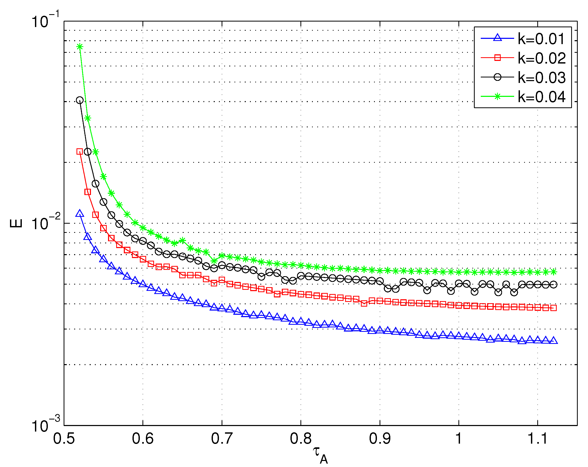
Figure 2.
RLBM simulation of a GSRDS, with spatially-varying parameters. The supply rate F and removal rate R are linear functions of the vertical and horizontal coordinate, respectively. The color map shows the order parameter , with red corresponding to values of and the deepest blue corresponding to . Also shown is the Hopf bifurcation (dotted line) and the saddle node bifurcation (solid line).

Figure 3.
Phase portraits of RLBM simulations of a GSRDS with different relaxation parameters

Figure 4.
Steady state flow and concentration fields of a TRLBM simulation in which chemical species A reversibly transforms into species B: , which has a lower enthalpy value (the reaction is exothermic in the forward direction). (a) Temperature field with velocity streamlines; (b) concentration field of the first component ; and (c) concentration field . The initial concentrations were .

Figure 5.
Heat flux components as a function of average chemical species concentration for TRLBM chemical convection simulations at two different Rayleigh numbers. The heat flux values (corresponding to diffusion in blue, convection in red and advection by passive scalar chemical species in green) are normalized by the total heat flux.
© 2017 by the author. Licensee MDPI, Basel, Switzerland. This article is an open access article distributed under the terms and conditions of the Creative Commons Attribution (CC BY) license (http://creativecommons.org/licenses/by/4.0/).
Share and Cite
MDPI and ACS Style
Bartlett, S. A Non-Isothermal Chemical Lattice Boltzmann Model Incorporating Thermal Reaction Kinetics and Enthalpy Changes. Computation 2017, 5, 37. https://doi.org/10.3390/computation5030037
AMA Style
Bartlett S. A Non-Isothermal Chemical Lattice Boltzmann Model Incorporating Thermal Reaction Kinetics and Enthalpy Changes. Computation. 2017; 5(3):37. https://doi.org/10.3390/computation5030037
Chicago/Turabian StyleBartlett, Stuart. 2017. "A Non-Isothermal Chemical Lattice Boltzmann Model Incorporating Thermal Reaction Kinetics and Enthalpy Changes" Computation 5, no. 3: 37. https://doi.org/10.3390/computation5030037
Note that from the first issue of 2016, this journal uses article numbers instead of page numbers. See further details here.