Time-Dependent Density-Functional Theory and Excitons in Bulk and Two-Dimensional Semiconductors

1
Department of Physics, University of Central Florida, Orlando, FL 32816-2385, USA
2
Department of Applied Physics, Aalto University, P.O. Box 11100, FI-00076 Aalto, Finland
*
Author to whom correspondence should be addressed.
Computation 2017, 5(3), 39; https://doi.org/10.3390/computation5030039
Submission received: 21 July 2017
/
Revised: 10 August 2017
/
Accepted: 15 August 2017
/
Published: 25 August 2017
(This article belongs to the Special Issue In Memory of Walter Kohn—Advances in Density Functional Theory)
Abstract
:In this work, we summarize the recent progress made in constructing time-dependent density-functional theory (TDDFT) exchange-correlation (XC) kernels capable to describe excitonic effects in semiconductors and apply these kernels in two important cases: a “classic” bulk semiconductor, GaAs, with weakly-bound excitons and a novel two-dimensional material, MoS2, with very strongly-bound excitonic states. Namely, after a brief review of the standard many-body semiconductor Bloch and Bethe-Salpether equation (SBE and BSE) and a combined TDDFT+BSE approaches, we proceed with details of the proposed pure TDDFT XC kernels for excitons. We analyze the reasons for successes and failures of these kernels in describing the excitons in bulk GaAs and monolayer MoS2, and conclude with a discussion of possible alternative kernels capable of accurately describing the bound electron-hole states in both bulk and two-dimensional materials.
1. Introduction
Accurate theoretical description of the optical properties of materials, especially semiconductors, is very important. From the practical side, these properties define the ability to absorb and emit light and many other features of the systems. Additionally, one needs to properly explain spectroscopic and other optical experimental data used to analyze the optical properties of materials. These properties are defined to a large degree by the excited states in the system, thus, it is very important to correctly describe the optical absorption spectrum that includes all possible types of excitations in order to understand the properties of the existing and predict the properties of new materials.
One of the greatest challenges in the case of semiconductors is proper description of the excitonic effects. Properties of the excitons, coupled one-electron, and one-hole states are, in principle, defined by many-body effects. In particular, the binding energy of the excitons and their size strongly depend on the static and dynamic screenings defined by the other charges, types of the atoms in the system and by their orbitals that accommodate the electrons and holes forming the exciton, etc. In most cases, especially for novel, complex, low-dimensional and nano-materials, it is not feasible to describe excitonic effects by using many-body theory or other phenomenological approaches, which generally have difficulties in taking all the important details described above into account. Therefore, it is very desirable to have proper ab initio tools capable of accurately describing excitonic effects in semiconductors [1].
The standard modern ab initio tool to study excitations in finite systems and solids is TDDFT [2], an effective theory of charge density, in which all effects of electron-electron interactions and, hence, all nontrivial excitations are described by the XC potential. Unfortunately, in the case of solids, standard TDDFT XC potentials, like adiabatic local density approximation (LDA) and generalized gradient approximation (GGA), do not give excitonic peaks in the absorption spectrum, or give such peaks with extremely small binding energies (see, e.g., [3,4,5]). Therefore, until very recent times the studies of excitons in semiconductors were almost universally based on a combined ab initio + many body approach, in which the GW calculations of the single-particle electronic structure were succeeded by calculations of the two-particle spectrum (that may include excitonic peaks) by solving the Bethe-Salpeter equation (BSE). This BSE approach [6,7,8] recommended itself as a reliable tool after being tested on many systems, though one also meets with difficulties when using it: large computational times, especially in the case of complex systems, not always well-adjusted approximations for the vertex function in solving the BS equation, etc. Thus, it would be very desirable to develop TDDFT XC potentials for excitons. Indeed, TDDFT is free from both shortcomings mentioned above—it is computationally much less expensive and is, in some sense, “exact”, i.e., one does not need to make any approximation for the XC potential. Since excitons can be considered within linear response theory, to study these excitations one basically needs only the linear part of the XC potential defined by the XC kernel.
The most straightforward way to calculate the TDDFT XC kernel for excitons is to obtain it from the BSE (see, e.g., [9,10,11])). This BSE XC kernel, as well as its derivative—the nanoquanta kernel [11,12]—showed themselves to be rather successful. However, extraction of these kernels requires almost the same computational efforts as to calculate the excitonic binding energies with the BSE approach. It is widely believed that one of the reasons of the successes of the BSE and nanoquanta kernels is that these functionals contain a Coulomb singularity responsible for the effective long-range electron-hole interaction necessary to form the Rydberg-type coupled electron-hole states. Then, one may naively expect that a phenomenological long-range (LR) kernel , with of the order of the inverse static dielectric constant for given material, can be chosen as a minimal model kernel to describe excitons [12,13,14]. Indeed, such a kernel was successfully applied to describe excitonic effects in bulk and 2D materials [4,5,15,16,17,18,19]. Unfortunately, the corresponding results strongly depend on the value of the parameter and the relation may not necessarily hold for all materials. Moreover, the strength of the oscillator peak (the peak height in the absorption spectrum) is often overestimated in the LR kernel solution. Moreover, it is doubtful that this kernel is capable of describing more “complicated” small-size, charge-transfer, excitons. Perhaps, in the last case semi-local, e.g., Tao-Perdew-Staroverov-Scuseria (TPSS) [20] or Tao-Mo (TM) [21] potentials, that accurately incorporate the short-range inhomogeneities, charge fluctuations, and other effects, have to be used.
On the other hand, one can consider more complex but parameter-free kernels with a Coulomb singularity, like the exact-exchange (EXX) kernel that can be derived from the exact-exchange energy. Goerling et al. [22,23] have derived the expression for such a kernel from the linear-response solution for the charge susceptibility. The EXX kernel was successfully applied in many cases (see, e.g., [24]). Alternatively, one can obtain such a kernel by performing straightforward differentiation of the energy functional with respect to the charge density. This procedure will give an equation for the XC potential, called the optimized effective potential (OEP) (for references and details, see, e.g., [25]). The last equation can be approximately solved and give the XC (for example, the Krieger-Li-Iafrate (KLI) [26]) potential and, subsequently, the XC kernel. The main disadvantage of the EXX, OEP, and similar potentials is their orbital dependencies, which significantly reduces the speed of the calculations.
Recently, an alternative LR, orbital-independent and parameter-free, bootstrap (BO) kernel was proposed in [27] and was successfully applied to several materials (see, e.g., [27,28,29]). The computational cost of the BO calculations is the same as those of ALDA, and the price can be reduced even further, by using a semi-analytical approximation in the BO equations, which give the random phase approximation BO (or RBO) kernel [30].
In this paper, we present details of the TDDFT formalism in the density-matrix representation (DM-TDDFT), and how it can be used to calculate the absorption spectrum and the excitonic binding energies in semiconductors. Beginning with the many-body (semiconductor Bloch equation and BSE) approach for excitons, we follow with details on the most often used approximations for the TDDFT XC kernels for excitons, including the contact, LR, and other kernels. In the last part of the work, we apply many of these kernels to two important materials: “classical” bulk semiconductor GaAs and a novel one-layer (1L) system of MoS2, [31] a system with very strong absorption and emission and strongly-bound excitons [31,32]. We discuss the reasons for the successes and failures of different kernels on the examples of these two representatives of the classes of the 2D and 3D materials, and argue how one can possibly improve the existing kernels for these two types of systems.
2. Charge Susceptibility, Absorption Spectrum and Excitons
Excitons are very often identified as isolated peaks below the conduction band edge in the experimentally-observed absorption spectrum. The last function can be calculated from the result for the charge susceptibility. In this section, we give details of the general scheme on how to calculate charge susceptibility within many-body theory and TDDFT and how to obtain the absorption spectrum using these functions. More details on this can be found, for example, in Ref. [25].
2.1. Many-Body Susceptibility
To calculate the charge susceptibility, let us begin with the formulation of general problem of linear response. In a perturbed system, one can separate the time-dependent charge density into the static (initial) and the perturbed (fluctuating) parts:
The space- and time-dependencies of the fluctuating part of the charge density are defined by the external potential:
where the first and the second parts are the static (including the ion) and the time-dependent (turned on at time ) parts of the potential, respectively. The second term defines also the interaction part of the many-body Hamiltonian operator in the Heisenberg representation:
where is the charge-density operator (here and below, the subscript 1 stands for the first-order, or linear, approximation). Part (3) of the total Hamiltonian defines the effects of the perturbation on the system ( is the Hamitonian of the unperturbed system). In order to find the charge susceptibility (and, hence, as we show below, the absorption spectrum), one does not need to solve the general nonequilibrium problem with the total, and usually a rather complicated, Hamiltonian . As an alternative, one can calculate the susceptibility within the linear-response approximation by finding first the eigenenergies and eigenfunctions from the solution of the static Schrödinger equation with the Hamiltonian . and define the charge susceptibility, or the retarded density-density response function:
where is the commutator of the density operators. The last function in frequency representation:
allows one to calculate the absorption spectrum (see Section 2.4).
In the linear-response approximation, the expression for the susceptibility also defines the density fluctuation as functional of the external potential:
i.e., Equations (4) and (5) completely define the excitation spectrum and the spatio-temporal charge dynamics.
To find the explicit frequency-dependent expression for the susceptibility (from Equation (5)), one can insert the sum of the product of eigenvectors (equal one) between the density operators in Equation (5), and then use the interaction representation for the density operators: on the right-hand side is time-independent), and use the fact that . This gives:
The last result can be also used to calculate the frequency-dependent fluctuating charge density from the frequency transform of Equation (6):
To summarize, knowledge of the eigenenergies and eigenfunctions of the unperturbed system allows one to calculate the charge susceptibility from Equation (7), which gives the excitation and absorption spectrum, including the excitonic peaks, and in general to obtain the linear-response charge dynamics from Equation (6) or Equation (8).
2.2. TDDFT Susceptibility
In TDDFT, the many-body problem is mapped on an effective problem of one electron in an “external” Kohn-Sham (KS) potential:
which is in general a non-linear functional of the charge density (the first, the second and the last terms on the right-hand side are the external, Hartree and the XC potentials, correspondingly). To find the linear-response TDDFT susceptibility, one can begin with substituting the linear (in external field and density) part of the KS “perturbing” potential into the linear-response TDDFT analogue of the many-body Equation (6):
where
is the KS susceptibility. The explicit expression for the linear KS XC potential is:
The only nontrivial (XC) part of the KS potential can be written as:
where
is the XC kernel, the key component of the TDDFT theory for excitons.
As the next step of the derivation of the equation for the susceptibility, one can substitute Equation (13) into Equation (12), and then Equation (12) into Equation (10), which gives:
Expressing the linear charge density in the last equation in terms of the susceptibility Equation (6) gives the TDDFT equation for the charge susceptibility in terms of the KS susceptibility and the XC kernel:
The KS susceptibility can be obtained from the static DFT results for the KS eigenfunctions and eigenenergies as:
where is the Fermi- or the highest-occupied molecular orbital energy and are the state occupancies (see Appendix A for the details of the derivation of the last equation).
Equation (16) can be also written in the frequency domain:
Then, inverting Equation (18) one may obtain the XC kernel in terms of the KS and total susceptibilities:
Thus, one can calculate the charge susceptibility from Equation (16) by using the static DFT result for the KS susceptibility (Equation (17)) and the TDDFT XC kernel. Provided the XC kernel has the proper form, one can obtain the exciton peaks in the absorption spectrum obtained from the susceptibility, as shown in Section 2.4.
2.3. Susceptibility: Finite vs. Extended (Periodic) Systems
The results obtained in the last two Subsections are valid in the general cases of finite systems and infinite non-periodic systems. In this subsection, we present the corresponding formula for the TDDFT susceptibility for periodic systems. In the last case, the problem is simplified, since one needs the KS eigenfunctions in the primitive cell only and the eigenvalues (band energies) are defined by the momenta in only one, the first, Brillouin zone.
Indeed, due to translation invariance of the response function:
( are lattice vectors) and of the other functions, like , and the Coulomb potential , one can express them as Fourier sums:
(and similar for and ) and:
where and are the reciprocal vectors. To simplify the expressions for the functions in the sums in the last equations, we introduce the definitions:
Substituting Equations (21)–(24) into Equation (18) gives the (reciprocal vector) matrix equation for the charge susceptibility:
where the frequency-dependent KS matrix susceptibility is defined as:
and are the band indices (for derivation of the last expression, see, for example [25]).
The solution of the matrix Equation (25) for (in practice, the equation is solved with a finite number of the reciprocal vectors that defines the rank of the matrices) basically consists of matrix inversion, and can be written as:
where
and:
(we have omitted the momentum and frequency indices , which are the same for each function and matrix in Equations (27)–(29)). The required number of the required reciprocal vectors is needed to be checked separately for each problem.
In the next subsection, we present details how one can obtain the absorption spectrum by using the susceptibilities from Equations (7), (18) and (27).
2.4. Absorption Spectrum
The absorption spectrum can be obtained by calculating the imaginary part of the macroscopic dielectric function that can be found by space-averaging the dielectric function . The last function is connected with the charge (optical) susceptibility from the previous subsections as:
In order to perform the macroscopic averaging of the last function, one can use the equation that connects the microscopic electric induction and the electric field by means of the dielectric function:
which, in the case of a periodic system, can be transformed to:
Averaging of the last equation over the unit cell gives the scalar relation between the macroscopic quantities:
In the homogeneous case, when , the dielectric function depends on the difference of two spatial vectors and its Fourier transform is diagonal in the reciprocal vector indices. In this case, the average of can be easily obtained by integrating over , which gives:
In the general, non-homogeneous, case due to local-field effects (spatial fluctuations), the situation is more complicated since is a non-diagonal matrix. In particular, in the case of cubic systems, to calculate , one needs to perform the matrix inversion (see, e.g., [33]):
In order to connect with the charge susceptibility matrix, one can write, in analogy with Equation (33), the equation:
Using Equation (6) gives:
In the periodic case, the last equation can be transformed to:
One can show from the last equation that the macroscopic dielectric function is:
where is calculated from Equation (25) with:
(for details of the derivation of Equation (38) and references, we refer the reader to Appendix M of [25]).
Thus, Equations (7), (18), (27) and (38) define the absorption spectrum. In the next section we begin to discuss the general features of different theories for excitons and how these features must be reflected in the structure of the XC kernel needed to obtain the absorption spectrum with excitonic peaks.
3. Many-Body Approaches for Excitons
3.1. Semiconductor Bloch Equations and the Wannier Equation
The simplest many-body approach for excitons is based on the single-particle approximation. Namely, one can consider the following two-band second quantized Hamiltonian of interacting quasi-particles in the Heisenberg representation for the operators [34]:
where and correspond to the electron and hole operators with the subscript momentum indices, are the electron and hole (conduction and valence band) spectra, is the Coulomb potential, is the pulse electric field and is the transition dipole moment (for simplicity, we omit the spin indices and vector symbols over the momentum and spatial vectors in this and/or some other large-size equations below). We use the dipole approximation for the interaction of the electrons and holes with the electric field, which is valid when the electric field wavelength is much larger than the unit cell and the magnetic component of the pulse can be neglected, like in the case of the visible light.
To analyze the response of the system to an external perturbation it is convenient to introduce the following quantities of interest that can be expressed in terms of averaged operators:
which correspond to the excited electron density, excited hole density and charge polarization (including excitonic states), respectively.
Writing down the Heisenberg equations for the operators under the average brackets in the last three equations, then statistically averaging the resulting equations, and making the Hartree-Fock splitting in the four-operator terms, one can get the semiconductor Bloch equations for the charge densities and the polarization:
where the last terms describe the scattering effects beyond the HF approximation. These equations allow one to find the time dependencies of the excited electron and hole densities, as well as the polarization. The last quantity in the frequency representation defines the absorption spectrum (see, e.g., [4]).
In the linear response theory approximation in the case of weak pulses one can put in these equations . Then, in the parabolic band approximation Equation (45) in the frequency representation transforms to:
where is the band gap energy and is the reduced electron-hole mass (we neglected the scattering effects beyond the HF approximation).
It is easy to see that the last equation reduces to the many-body Wannier equation for the excitons [35] if one neglects the (source) term on its right-hand side. The solution of the Wannier equation gives the energy of exciton—a coupled state of electron and hole that interact with the Coulomb potential . Thus, the polarization has a pole at the excitonic energy within the band gap, and hence the absorption spectrum possesses a peak at this energy. In principle, one can use the solution of Equation (48) to estimate the exciton energies in solids by adding a dielectric (screening) parameter in front of the Coulomb potential, though in many cases such an approximation, which neglects details of the dynamical and local-field effects, is not sufficient.
3.2. Bethe-Salpeter Equation
A higher level of the many-body approximation to study excitons is based on the Bethe-Salpeter equation (BSE) approach [6,7,8]. In this case, to describe the two-particle effects, including excitons, along with the one-particle Green’s function (GF):
and one also finds the two-particle GF:
where is the time-ordering operator. For simplicity, in the last two equations we use one lower index for the electron operator, that corresponds to the space and time coordinates and the electron quantum numbers, like momentum, orbital momentum and spin. While the one-particle GF describes the single-particle properties, the two-particle one contains information about the energies of the two-particle states, including excitons, and other two-particle properties of the system.
Formally, the solution for the two-particle GF can be expressed in terms of one-particle GFs as:
where is a reducible kernel and summation (integration) over repeated indices is assumed (for details, see, e.g., [36]).
For the reasons given below, it is more convenient to use an irreducible kernel instead of the reducible one (the irreducible kernel, contrary to the second one, does not include diagrams that can be divided by cutting two single-particle GF lines). Both kernels are connected by the following relation:
Using the irreducible kernel, one can write an equation for another GF:
This equation is:
Equations (52) and (54) are called the Bethe-Salpeter equations for the reducible kernel and for the Green’s function , correspondingly.
There are several advantages of using the function instead of . The first one is that one can easily find the charge susceptibility from :
(the upper plus signs mean that the time for the corresponding operators is larger by an infinitesimally small amount than in the corresponding operator without this sign). Another important advantage is the possibility to calculate the excitonic spectrum from Equation (54). Let us demonstrate this.
Assuming the Coulomb interaction to be weak, and expanding the two-particle GF on the left-hand side of Equation (51) in the lowest-order approximation in the Coulomb interaction , one can obtain the lowest order in approximation for . Then, substitution of into Equation (52) allows one to find the lowest-order expression for :
Substituting this result into Equation (54), approximating the single-particle GFs in the last equation by their free-electron counterparts , putting the time variables equal and and performing the frequency Fourier transform with respect to the time variable , one can modify Equation (54) to:
where (detailed expression for this function is given in Equation (58) below).
To show explicitly that the function defined in Equation (57) contains the necessary information about the excitons, we will transform the last equation into an equation that looks more similar to the familiar excitonic Wannier equation (Equation (48)). For this, the following steps need to be taken. First, one transforms the time-ordered GFs into the retarded ones using the Langreth’s rules [36]. Second, using the Lehmann’s representation for the free GFs one can express them in terms of the DFT KS wave functions and energies. This, in particular, gives:
As the next step, one can look for the solution for the GF L by using the following approximation (ansatz):
Finally, substituting this expression into Equation (57), one can obtain two equations for the unknown “excitonic” matrix elements and . In the case of applied pulse with frequency close to the gap frequency, one can show that , i.e., can be neglected (this corresponds to the Tamm-Dancoff approximation). This can be seen by looking at the pole structure of these two functions at frequencies close to the gap value: , .
Thus, the remaining equation in momentum representation becomes:
i.e., it has the form of the Wannier Equation (48). Therefore, function and hence the two-particle GF (54) has an excitonic pole(s) (for more details of the derivation, see book [36]). In practice, however, one needs to solve the original Equation (57) more accurately to obtain the excitonic binding energies in the BSE formalism.
4. TDDFT and Excitons: the Density-Matrix Approach
To begin, the discussion on studies of excitons with “pure” TDDFT, we present the DM formulation of this theory [4,5,19], which is one of the most convenient schemes for the practical applications. To derive the DM-TDDFT equation for the exciton binding energy, one can begin with the KS equation:
where k is the wave vector, v is the valence-band index, and the KS Hamiltonian is:
In the last equation, the terms on the right-hand side are the kinetic (first), Hartree (second), and XC (third) potentials, and an external homogeneous electric field (the last term). Equation (61) has to be solved self-consistently with the equation for the electron density:
where are the occupied band indices. In the DM representation, Equations (61) and (62) are solved by expanding the KS wave function in the basis of the static DFT wave functions :
The time-dependent coefficients completely describe the system dynamics. Below we drop index v for sake of simplicity, since we will consider the case of one valence band. The coefficients can be found from the following equation:
where
However, to study the system response it is more convenient to consider the bilinear combination of c-coefficients, the density matrix:
Its diagonal elements describe the level occupancies, while the non-diagonal ones—the electron transitions, including the excitonic effects. The matrix elements satisfy the Liouville equation:
In the case of two (valence v and conduction c) bands, one can derive the exciton TDDFT equation for the non-diagonal element by using Equations (62), (63), (66) and (68). Expansion of the charge density fluctuations in Equation (68), in terms of the density matrix elements (Equation (67)) (by using Equation (63)), leads to the TDDFT Wannier equation [5]:
where q is the exciton momentum, α is the reduced hole mass, and n is the bound state number. The effective electron-hole interaction is described by the last term in the brackets defined as:
One can obtain the excitonic binding energies from Equation (69) by setting q = 0.
We have generalized the above formalism for the case of higher excitations—trions and biexcitons [19]. One can derive equations for these quasi-particles similar to Equation (69) by expanding the corresponding wave functions in terms of three (trion) and four (bi-exciton) KS wave functions with the coefficients that include the corresponding polarization matrix elements. The solution of the equation for this element will give the binding energy for the trion and biexciton. In addition to the e-h attraction terms of type (69), and the equation will also include the e-e and h-h repulsion terms with the interaction matrix elements:
( is static e-e screening; for details, see [19]).
In the following Subsections we present an overview of the main types of the proposed kernels to study excitons with TDDFT. To calculate the excitonic energy one can proceed in three ways:
- (1)
- to calculate the dielectric function with a given fxc, as described in Section 2. Then, the excitonic binding energies will be identified as peaks in the absorption spectrum.
- (2)
- to propagate in time the KS equation, with consequent frequency transformation of the polarization matrix element which also defines the absorption spectrum that might include excitonic peaks.
- (3)
- to solve the linearized Equation (69) for the excitonic binding energies.
The first and the third approaches correspond to the linear response (where the XC kernel is used), while the second might be regarded as a more general, since the time-propagation of the KS equation can be performed for any non-linear XC potential.
Below, we describe the main types of proposed XC kernels which we will use to calculate the excitonic binding energies with Approach 3.
5. XC Kernels
5.1. BSE Kernel: General Definition and the Nanoquanta Approximation
The most straightforward and most formal way to analyze the structure of the XC kernel for excitons would be to start from the BSE (Equation (54)). Namely, one can derive the equation for the charge susceptibility from Equation (54) by using the variables for the function L as in Equation (55) and compare the resulting equation with the corresponding TDDFT (Equation (18)) in order to obtian the structure of the BSE fxc. After some straightforward but cumbersome transformations, the combination of these two equations give the following equation that connects the XC kernel with the reducible kernel K:
In some sense, it is meaningless to apply the BSE XC kernel to study the excitons with TDDFT, since the solution of the BSE equation along with the XC kernel provides also the excitonic energies (as poles of the charge susceptibilities, Equation (55)). However, the knowledge of the structure of the BSE XC kernel for excitons is very important from the point of view of building the general TDDFT for semiconductors.
Below, we briefly describe one possible approximation for the solution of Equation (72), which gives the so-called nanoquanta XC kernel [12]. In this approximation, one first finds the many-body single (quasi)-particle GF by using the lowest-order GW approximation for the electron self-energy, , where the screened Coulomb interaction is defined by the equation:
where ( is the irreducible susceptibility). Then, using the one-loop approximation (the first term in Equation (54)) for and on the r.h.s. of Equation (72) and the one-loop approximation for the susceptibilities on the l.h.s. of this equation, , one can obtain an equation for the part of the XC kernel that produces excitonic states:
with the screened interaction defined by Equation (73), where one sets . This kernel was successfully applied to study the excitonic effects in different materials, including Si [3] and Ar [10].
5.2. Adiabatic Local XC Kernels
In the adiabatic approximation, all memory effects are neglected. To get an excitonic state, the memory effects do not appear to be decisive, though they can significantly modify the binding energy. The simplest adiabatic XC kernel is the adiabatic (local-in-time) spatially-independent contact kernel:
where A describes the effects of local charge “interaction”. Being purely phenomenological, this kernel can capture the main features of the excitonic effects in some materials. Indeed, one can regard it as averaged over cell more realistic adiabatic LDA XC kernel:
or even more complex gradient density-corrected kernels, like gradient-expansion approximation (GEA), Perdew-Wang (PW91) [37], Perdew-Burke-Ernzernhof (PBE) [38], and other GGA kernels (see [25] for details on the kernels and the references).
As a rule, the LDA, PBE and other local kernels lead to strongly underestimated binding energies. This is connected with neglecting the LR (Coulomb) features in the e-h interaction, since the Coulomb interaction is needed for strong binding of the usually far-separated electrons and holes.
5.3. Adiabatic LR XC Kernels
Indeed, taking into account effects of LR interaction improves significantly the situation, the binding energies are often of order of the experimentally-observed values.
The simplest LR kernel is the kernel with the same name:
where is the effective scattering parameter (dielectric function).
More systematically one can construct an XC kernel that takes into account the effects of the LR interaction by using an energy functional that includes such effects. A natural choice for such a functional is the exact exchange (EXX) energy:
where is the spin variable and and are other quantum numbers that correspond to given state. Since the corresponding XC potential (OEP [39,40]) and the kernel depend on the set of orbitals, to obtain the XC potential one needs to perform the functional differentiation of the energy (Equation (78)) by using the chain rule, which can be symbolically written as . Performing the differentiation and applying some other transformations in the resulting equation will lead to the following equation for :
where
The fist summation in Equation (79) is performed over the occupied states, while the last one—over all states. Since one cannot invert Equation (79) in order to obtain the explicit analytical expression for the XP potential (though the exact potential can be obtained numerically [41]), to get a feeling of the main features of the OEP potential one needs to transform the equation to a more convenient form by doing some approximations. The simplest one, the so called KLI approximation, [26] is based on approximating the energy differences in this equation by the effective average value . In this case, the equation is significantly simplified:
with:
While it is much easier to solve the KLI (Equation (81)) than the general OEP (Equation (79)), in practice some additional approximations in the KLI equation are often used. One of them is to neglect the spatially-independent term under the integral , which gives the Slater XC potential:
Further simplification is the approximation of the orbital charge density in the denominator of the last expression by the average value, which gives the global averaging method (GAM) XC potential:
Using the differentiation chain rule in Equations (81), (83) and (84) as above, one can obtain the expressions for the KLI, Slater, and GAM XC kernels, correspondingly (actually, in the KLI case—the equation for the kernel). We present here the expressions for the Slater kernel:
As it follows from the results above, the three kernels contain the Coulomb singularity, which results in a rather good description of the exciton energies even in the GAM case.
5.4. Exact-Exchange (Frequency-Dependent) Kernels
Another example of the LR kernel which includes also non-adiabatic effects is the EXX kernel. As it was shown by Goerling et al. [22,23] using the exact exchange energy and deriving the linear response charge susceptibility, such a kernel has the following structure:
where is a functional of the Coulomb potential and of the KS wave functions that contains the Coulomb singularity core . This core results in a singular structure of the kernel in the momentum representation. In particular, the lowest in the reciprocal vector indices part of the XC kernel matrix has the following singular form:
As the calculations show, the presence of the Coulomb singularity leads to a rather successful description of the excitonic effects in some materials when the momentum cut-off is enforced (see, e.g., [24]).
5.5. Semi-Local Approximation: Tao-Mo Kernel
There is another possible type of the non-local XC potential for excitons that properly takes into account short-range interaction effects—the so-called semi-local potentials (and, hence, semi-local kernels). These potentials might be relevant in the case of small-radius, e.g., charge-transfer, excitons. We will stop on one such a recently proposed potential by Tao and Mo (TM) [21] that gives improved XC energy as compared to LDA, PBE, and TPSS potentials. The derivation of the expression for the exchange hole for the TM potential was based on the second-order expansion in small (non-locality) parameter and assuming that the result: (1) recovers the uniform electron gas case; (2) gives the correct small dependence up to the second-order expansion; (3) gives a converged large limit.
More precisely, starting from general expression that connects the exchange energy and the hole:
using the conventional hole , introducing new variables and , where is a contraction parameter, expanding the hole in terms of small u, and averaging the integral in Equation (88) over u, one can arrive to the following expression for the XC energy that is a local functional of the charge density and its and corrections. The advantage of this type of functional is its locality, and on the other hand ability to take into account short-range (charge fluctuation/non-locality) effects. We refer the reader to [21] for discussion on how the non-local effects on the semi-local level lead to an improvement of the system energies as compared to the LDA and other local potentials.
5.6. Bootstrap Kernel
Another type of kernel that takes into account the effects of long-range interaction and is physically motivated by its close connection to the experimental quantity–dielectric function, the so called Bootstrap (BO) kernel was proposed by Gross and collaborators [27]. The basic motivation for the choice of the kernel was that: (1) it must have a Coulomb singularity, , in which case the dielectric function may have an exciton pole at finite frequency; and (2) at the kernel gives static dielectric function close to RPA, that reproduces the experimental data well.
The postulated kernel has the following structure:
where the KS susceptibility and the dielectric function are defined in Equations (26) and (38), correspondingly. To find the kernel (Equation (89)) one has to solve the last equation self-consistently with Equations (25) and (38) for the susceptibility and dielectric functions.
A significant advantage of the BO kernel is its genuinely “ab initio” form (i.e., it is essentially defined by the KS wave functions), relative technical simplicity of calculation as compared, e.g., to the the EXX kernel. As results of the calculations show, the BO kernel can successfully describe excitonic effects for a large number of bulk semiconductors.
5.7. RPA Bootstrap (RBO) Kernel
Simplification of the BO kernel leads to the so called RPA Bootstrap (RBO) [30] kernel constructed by approximating the macroscopic dielectric function by its 00 matrix element in the reciprocal vector representation:
Then, one transforms the susceptibility equation into the macroscopic and the RPA parts:
where is the Coulomb potential (Equation (40)).
Next, substitution of the macroscopic dielectric function (Equation (90)) into the BO XC kernel Equation (89) gives:
In the RBO approximation, only the terms with are taken into account. Contrary to the BO case, where one needs to iterate the system of Equations (25), (38) and (48), in the RBO approximation one does not need to do it. Namely, the analytical solution of the corresponding system of Equations (90)–(93) gives:
To find the RBO kernel, one needs to calculate from Equation (26), then from Equation (92), substitute these two into Equation (94) and the resulting and in Equation (93).
In fact, one can find the exciton energy even without using the XC kernel in this case: the exciton pole occurs at frequency when , and hence , (see Equation (90)) has a pole inside the gap. This is a great simplification of the RBO approximation which, in many cases, give similar results to the BO absorption spectrum (for a recent discussion on the connections between both kernels, see [42,43]).
6. Applications: Bulk GaAs and Monolayer MoS2
6.1. GaAs
The DFT part of the calculations was performed with the plane-wave and pseudopotential method as implemented in the Quantum Espresso package [44]. The PBE XC potential [38] was used to take into account the effects of the electron interaction, and the ultra-soft pseudopotentials were used to describe the core-valence charge interactions. For all results presented, the energy cutoffs of 65 Ry and 360 Ry were used for the plane-wave basis sets and the charge density grids, respectively. These settings have been verified to achieve the total energy convergence less than 0.0001 a.u. For geometry relaxation, the force on atoms is converged below the threshold of 0.001 a.u. We have used the mesh for the k-points in the first Brillouine zone.
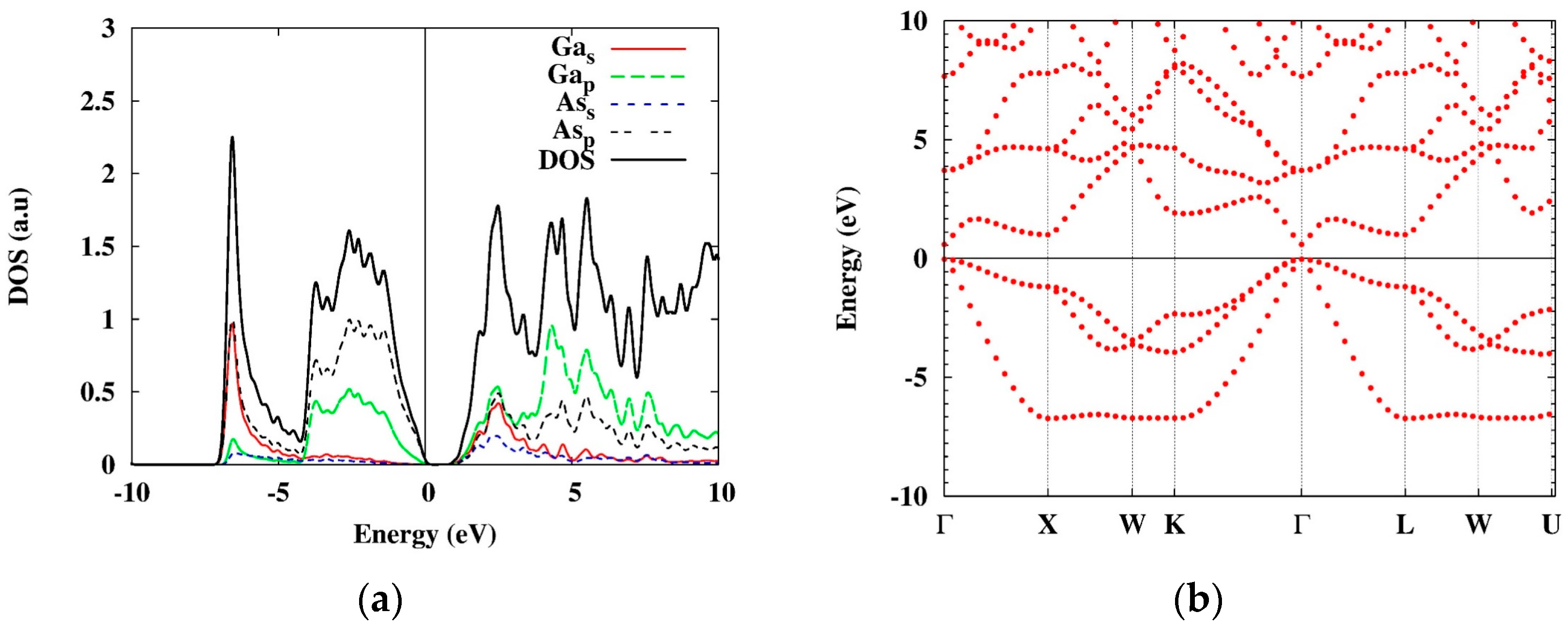
The primitive cell of the system and the orbital densities of GaAs are shown in Figure 1, and for the corresponding atomic DOS and the band structure—see Figure 2.
As it follows from these figures, there are two heavy- and one light-hole bands near the gamma-point. The heavy-hole band is doubly degenerate at this point (we will mark the corresponding states hh1, hh2, and lh, correspondingly). Thus, we will consider three types of excitons corresponding to the three types of holes. For simplicity, we neglect here the effects of the spin orbit splitting which do not significantly affect the excitonic binding energies.
Using this DFT input data, we have calculated the excitonic binding energies by solving eigen-energy Equation (69) in the two-band approximation. The results for the corresponding excitonic energies obtained with the local and the LR kernels are shown in Table 1.
As follows from Table 1, the local kernels severely underestimate the values for the excitonic binding energies, while the LR kernels are in reasonable agreement with the experimental data.
It is important to note that no bound states were found in GaAs (see, e.g., [41,47]) with LDA and some GGA potentials. Our very small binding energies (<0.5 meV) for GaAs is almost in agreement with these theoretical results, taking into account difference in the DFT input used in the TDDFT calculations. Similar conclusion can be made in the case of the Slater kernel. Namely, our result of rather weakly-bound electron-hole states (energy ~1 meV) and the absence of binding found in [41] can be possibly due to the arguments above and also due to different number of the occupied bands used in the DFT calculations that define the total ground state charge density that enters in the Slater XC kernel. In particular, in the Quantum Expresso code that we used, this number is different for the LDA (used in the work [41]) and PBE (used by us) pseudopotential files.
As it was mentioned above, the main reason for the failure of the local kernels is the missing LR feature in their structure. Inclusion of the correlation energy correction (in the PW interpolated approximation, Ref. [37] defined as “PW corr” in Table 1) does not improve the situation. Moreover, from Table 1 it follows that the exchange-part of the kernel gives the main contribution to the electron-hole coupling. Importantly, the inclusion of the semi-local correction (TM kernel) significantly improves the values of the excitonic energies (0.6 meV, 0.5 meV, and 0.8 meV for three states in Table 1) as compared to the local kernel results, though the numbers are still significantly lower than the experimental ones. The main reason for this is large excitonic radii in GaAs, and in such distances the semi-local corrections do not work sufficiently well.
We find that the BO kernel with its LR structure gives the excitonic binding energy 1 meV for the strongest bound that is of the same order of magnitude as in the experimental data. Detailed analysis of the dependence of the excitonic energies on the number of k-points and other computational parameters in the LR and BO kernels were performed in [48,49]. Our result for the LR kernel are in a reasonable agreement with those in [48,49] (0.5 meV vs. 0.6–0.8 meV), especially given the difference in the screening dielectric constant parameters (we used , while smaller values were used in [48,49]). For the BO kernel our result of 1 meV is in slightly better agreement with experiment than the one obtained in [49] (~0.3 meV). As shown also in [49], one can obtain binding energies from the BO kernel which are closer to experimental values by performing a material-dependent scaling of the dielectric function.
6.2. MoS2
Similar to GaAs, the DFT part of the calculations was performed by using the Quantum Espresso package [44] with PBE XC potential [38] and ultra-soft pseudopotentials. The energy cutoffs are 65 Ry and 360 Ry for the plane-wave basis sets and the charge density grids, respectively, and the mesh for the k-points in the first Brillouine zone was used.
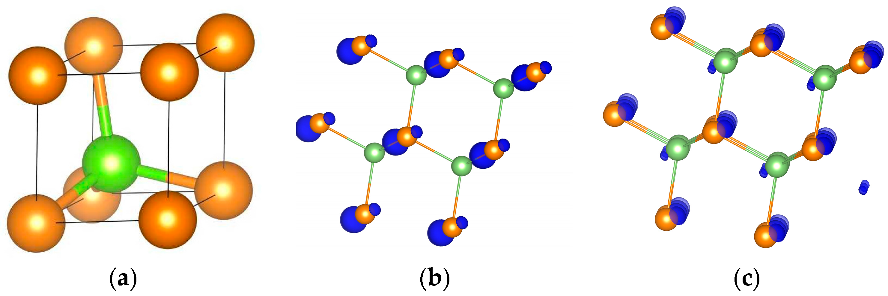
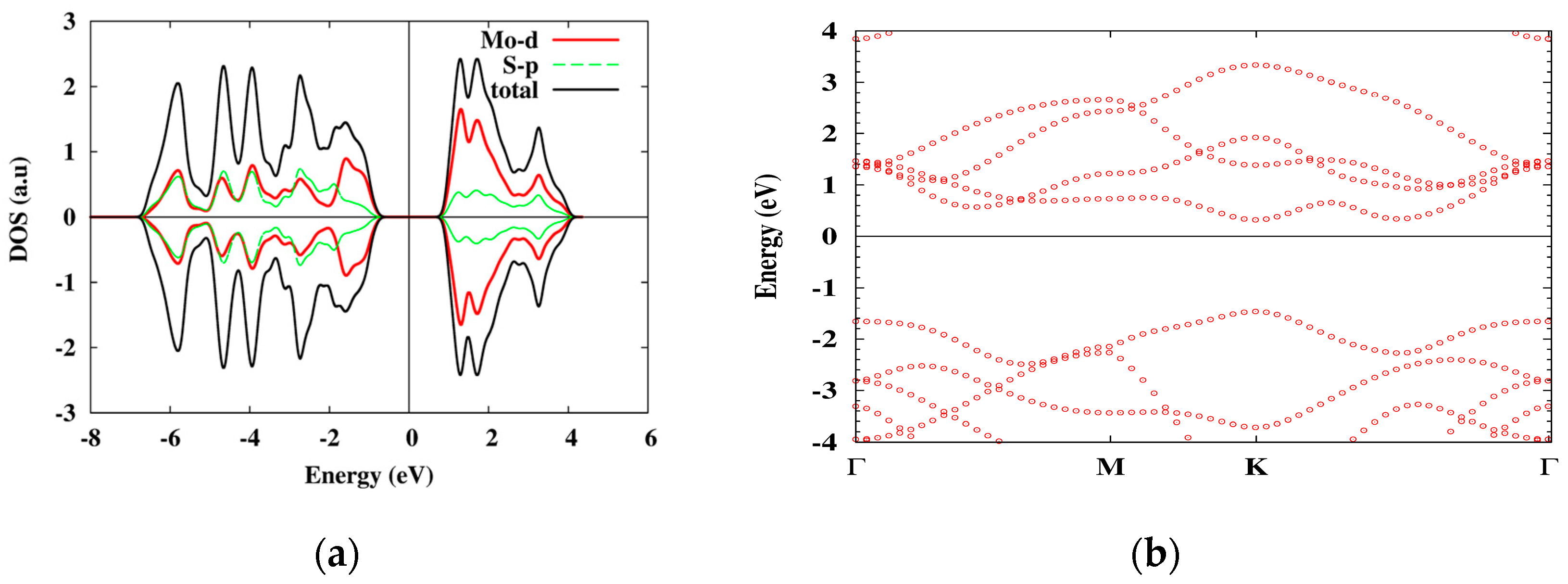
As DFT calculations show, the material is a direct-gap semiconductor, with dominating Mo atom d-orbital contribution to the excited electron and hole states (the lattice and the electronic band structures are shown in Figure 3 and Figure 4, correspondingly). The two-dimensional structure of the system results in a strongly reduced e-h screening which lead to large excitonic energies.
Similar to GaAs, the LR kernels do much better job giving excitonic energies that are not far from the experimental estimations 0.2–0.5 eV [31,32] (Table 2). It is important to stress that the results obtained with the local and LR kernel strongly depend on the choice of parameters, and one can reproduce the experimental data with reasonable choice of and .
Importantly, the semi-local correction for this material (TM XC kernel) significantly improves the value of the binding energy (81 meV) as compared to, for example the LDA kernel result (9.6 meV). The possible reason for better performance of the semi-local kernel in the case of MoS2 as compared to GaAs is much smaller (~10 times) excitonic radius in MoS2 (~100 A in GaAs). The BO kernel result is also in rather good agreement with the experiment—0.15 eV.
7. Discussion
In this work we discussed details of the most often used many-body and TDDFT approaches to study excitonic effects in semiconductors. We paid special attention to the structure of relevant TDDFT XC kernels and applied many of them to two different systems: bulk GaAs and monolayer MoS2. As our results show, the kernels that contain Coulomb singularity (LR, Slater, BO) produce excitonic energies much closer to that extracted from experimental data than the local kernels. The conclusion is valid for both materials. On the other hand, we found that the semi-local correction (the TM kernel) leads to significant improvement of the result in the case of MoS2 because of the smaller excitonic radius in this system.
These and other recent results demonstrate that TDDFT is a good, inexpensive alternative to the BSE approach to study excitonic effects in semiconductors. Nevertheless several important steps still need to be performed, such as:
- (1)
- Construction of kernels that can reproduce accurately exciton (not-necessarily) Rydberg series. For this, frequency-dependence of the kernel might be crucial.
- (2)
- Description of excitons with different spins (dark and bright excitons, etc.). In this case spin TDDFT must be considered, together with possible spin-dependent kernels (matrices).
- (3)
- Accurate description of the excitonic time-resolved emission spectra, in which phonon effects must be taken into account. In this sense, for practical purposes it would be desirable to construct a non-adiabatic kernel that incorporates memory effects related to electron-phonon interaction.
Solutions of these problems will, hopefully, lead us closer to a complete TDDFT for excitons.
Acknowledgments
We thank DOE for partial support under grant DOE-DE-FG02-07ER46354.
Author Contributions
T.S.R. guided the project. N.U.D. and V.T. performed the calculations. V.T., N.U.D. and T.S.R. analyzed and discussed the results and contributed to the writing of the manuscript.
Conflicts of Interest
The authors declare no conflict of interest.
Appendix A. Kohn-Sham Response Function
Let us find the KS susceptibility by expressing it in terms of the one-particle GFs.
We begin with the retarded and advanced GF operators:
that give the corresponding GFs:
For the lesser Green’s function the fluctuation-dissipation theorem:
Gives:
In our case, , , and one obtains:
Thus, from Equation (A7) one can obtain:
which coincides with Equation (17).
References
- Onida, G.; Reining, L.; Rubio, A. Electronic excitations: Density-functional versus many-body Green’s-function approaches. Rev. Mod. Phys. 2002, 74, 601. [Google Scholar] [CrossRef]
- Runge, E.; Gross, E.K.U. Density-functional theory for time-dependent systems. Phys. Rev. Lett. 1984, 52, 997. [Google Scholar] [CrossRef]
- Botti, S.; Schindlmayr, A.; Del Sole, R.; Reining, L. Time-dependent density-functional theory for extended systems. Rep. Prog. Phys. 2007, 70, 357. [Google Scholar] [CrossRef]
- Turkowski, V.; Ullrich, C.A. Time-dependent density-functional theory for ultrafast interband excitations. Phys. Rev. B 2008, 77, 075204. [Google Scholar] [CrossRef]
- Turkowski, V.; Leonardo, A.; Ullrich, C.A. Time-dependent density-functional theory approach for exciton binding energies. Phys. Rev. B 2009, 79, 233201. [Google Scholar] [CrossRef]
- Hanke, W.; Sham, L.J. Many-particle effects in the optical spectrum of a semiconductor. Phys. Rev. B 1980, 21, 4656. [Google Scholar] [CrossRef]
- Albrecht, S.; Reining, L.; Del Sole, R.; Onida, G. Ab Initio Calculation of Excitonic Effects in the Optical Spectra of Semiconductors. Phys. Rev. Lett. 1998, 80, 4510. [Google Scholar] [CrossRef]
- Rohlfing, M.; Louie, S.G. Electron-Hole Excitations in Semiconductors and Insulators. Phys. Rev. Lett. 1998, 81, 2312. [Google Scholar] [CrossRef]
- Von Barth, U.; Dahlen, N.E.; van Leeuwen, R.; Stefanucci, G. Conserving approximations in time-dependent density functional theory. Phys. Rev. B 2005, 72, 235109. [Google Scholar] [CrossRef]
- Sottile, F.; Olevano, V.; Reining, L. Parameter-Free Calculation of Response Functions in Time-Dependent Density-Functional Theory. Phys. Rev. Lett. 2003, 91, 056402. [Google Scholar] [CrossRef] [PubMed]
- Marini, A.; Del Sole, R.; Rubio, A. Bound Excitons in Time-Dependent Density-Functional Theory: Optical and Energy-Loss Spectra. Phys. Rev. Lett. 2003, 91, 256402. [Google Scholar] [CrossRef]
- Reining, L.; Olevano, V.; Rubio, A.; Onida, G. Excitonic Effects in Solids Described by Time-Dependent Density-Functional Theory. Phys. Rev. Lett. 2002, 88, 066404. [Google Scholar] [CrossRef] [PubMed]
- Botti, S.; Sottile, F.; Vast, N.; Olevano, V.; Reining, L.; Weissker, H.-C.; Rubio, A.; Onida, G.; Del Sole, R.; Godby, R.W. Long-range contribution to the exchange-correlation kernel of time-dependent density functional theory. Phys. Rev. B 2004, 69, 155112. [Google Scholar] [CrossRef]
- Botti, S.; Fourreau, A.; Nguyen, F.; Renault, Y.-O.; Sottile, F.; Reining, L. Energy dependence of the exchange-correlation kernel of time-dependent density functional theory: A simple model for solids. Phys. Rev. B 2005, 72, 125203. [Google Scholar] [CrossRef]
- Sottile, F.; Karlsson, K.; Reining, L.; Aryasetiawan, F. Macroscopic and microscopic components of exchange-correlation interactions. Phys. Rev. B 2003, 68, 205112. [Google Scholar] [CrossRef]
- Wełnic, W.; Botti, S.; Reining, L.; Wuttig, M. Origin of the Optical Contrast in Phase-Change Materials. Phys. Rev. Lett. 2007, 98, 236403. [Google Scholar] [CrossRef] [PubMed]
- Zhang, G.-X.; Tkatchenko, A.; Paier, J.; Appel, H.; Scheffler, M. Van der Waals Interactions in Ionic and Semiconductor Solids. Phys. Rev. Lett. 2011, 107, 245501. [Google Scholar] [CrossRef] [PubMed]
- Hübener, H.; Luppi, E.; Véniard, V. Ab initio calculation of many-body effects on the second-harmonic generation spectra of hexagonal SiC polytypes. Phys. Rev. B 2011, 83, 115205. [Google Scholar] [CrossRef]
- Ramirez-Torres, A.; Turkowski, V.; Rahman, T.S. Time-Dependent density-matrix functional theory for trion excitations: Application to monolayer MoS2 and other transition-metal dichalcogenides. Phys. Rev. B 2014, 90, 085419. [Google Scholar] [CrossRef]
- Tao, J.; Perdew, J.P.; Staroverov, V.N.; Gustavo, E.; Scuseria, G.E. Climbing the Density Functional Ladder: Nonempirical Meta–Generalized Gradient Approximation Designed for Molecules and Solids. Phys. Rev. Lett. 2003, 91, 146401. [Google Scholar] [CrossRef] [PubMed]
- Tao, J.; Mo, Y. Accurate Semi-Local Density Functional for Condensed-Matter Physics and Quantum Chemistry. Phys. Rev. Lett. 2016, 117, 073001. [Google Scholar] [CrossRef]
- Kim, Y.-H.; Görling, A. Excitonic Optical Spectrum of Semiconductors Obtained by Time-Dependent Density-Functional Theory with the Exact-Exchange Kernel. Phys. Rev. Lett. 2002, 89, 096402. [Google Scholar] [CrossRef] [PubMed]
- Kim, Y.-H.; Görling, A. Exact Kohn-Sham exchange kernel for insulators and its long-wavelength behavior. Phys. Rev. B 2002, 66, 035114. [Google Scholar] [CrossRef]
- Bruneval, F.; Sottile, F.; Olevano, V.; Reining, L. Beyond time-dependent exact exchange: The need for long-range correlation. J. Chem. Phys. 2006, 124, 144113. [Google Scholar] [CrossRef] [PubMed]
- Ullrich, C.A. Time-Dependent Density-Functional Theory: Concepts and Applications, 1st ed.; Oxford University Press: Oxford, UK, 2011. [Google Scholar]
- Krieger, J.B.; Li, Y.; Iafrate, G.J. Construction and application of an accurate local spin-polarized Kohn-Sham potential with integer discontinuity: Exchange-only theory. Phys. Rev. A 1992, 45, 101. [Google Scholar] [CrossRef] [PubMed]
- Sharma, A.; Dewhurst, J.K.; Sanna, A.; Gross, E.K.U. Bootstrap Approximation for the Exchange-Correlation Kernel of Time-Dependent Density-Functional Theory. Phys. Rev. Lett. 2011, 107, 186401. [Google Scholar] [CrossRef]
- Sharma, A.; Dewhurst, J.K.; Sanna, A.; Rubio, A.; Gross, E.K.I. Enhanced excitonic effects in the energy loss spectra of LiF and Ar at large momentum transfer. New J. Phys. 2012, 14, 053052. [Google Scholar] [CrossRef]
- Yang, Z.-H.; Li, Y.; Ullrich, C.A. A minimal model for excitons within time-dependent density-functional theory. J. Chem. Phys. 2012, 137, 014513. [Google Scholar] [CrossRef] [PubMed]
- Rigamonti, S.; Botti, S.; Veniard, V.; Draxl, C.; Reining, L.; Sottile, F. Estimating Excitonic Effects in the Absorption Spectra of Solids: Problems and Insight from a Guided Iteration Scheme. Phys. Rev. Lett. 2015, 114, 146402. [Google Scholar] [CrossRef] [PubMed]
- Mak, K.F.; Lee, C.; Hone, J.; Shan, J.; Heinz, T.F. Atomically Thin MoS2: A New Direct-Gap Semiconductor. Phys. Rev. Lett. 2010, 105, 136805. [Google Scholar] [CrossRef] [PubMed]
- Wu, F.; Qu, F.; MacDonald, A.H. Exciton band structure of monolayer MoS2. Phys. Rev. B 2015, 91, 075310. [Google Scholar] [CrossRef]
- Del Sole, R.; Fiorino, E. Macroscopic dielectric tensor at crystal surfaces. Phys. Rev. B 1984, 29, 4631. [Google Scholar] [CrossRef]
- Haug, H.; Koch, S.W. Quantum Theory of the Optical and Electronic Properties of Semiconductors; World Scientific Publishing Co., Inc.: Singapore, 2009. [Google Scholar]
- Wannier, G.H. The Structure of Electronic Excitation Levels in Insulating Crystals. Phys. Rev. 1937, 52, 191. [Google Scholar] [CrossRef]
- Stefanucci, G.; van Leeuwen, R. Nonequilibrium Many-Body Theory of Quantum Systems: A Modern Introduction, 1st ed.; Cambridge University Press: Cambridge, UK, 2013. [Google Scholar]
- Perdew, J.P.; Wang, Y. Accurate and simple analytic representation of the electron-gas correlation energy. Phys. Rev. B 1992, 45, 13244. [Google Scholar] [CrossRef]
- Perdew, J.P.; Burke, K.; Ernzerhof, M. Generalized Gradient Approximation Made Simple. Phys. Rev. Lett. 1996, 77, 3865. [Google Scholar] [CrossRef] [PubMed]
- Talman, J.D.; Shadwick, W.F. Optimized effective atomic central potential. Phys. Rev. A 1976, 14, 36. [Google Scholar] [CrossRef]
- Norman, M.R.; Koelling, D.D. Towards a Kohn-Sham potential via the optimized effective-potential method. Phys. Rev. B 1984, 30, 5530. [Google Scholar] [CrossRef]
- Yang, Z.-H.; Ullrich, C.A. Direct calculations of exciton binding energy with time-dependent density-functional theory. Phys. Rev. B 2013, 87, 195204. [Google Scholar] [CrossRef]
- Sharma, A.; Dewhurst, J.K.; Sanna, A.; Gross, E.K.U. Comment on “Estimating Excitonic Effects in the Absorption Spectra of Solids: Problems and Insight from a Guided Iteration Scheme”. Phys. Rev. Lett. 2016, 117, 159701. [Google Scholar] [CrossRef]
- Rigamonti, S.; Botti, S.; Veniard, V.; Draxl, C.; Reining, L.; Sottile, F. Reply. Phys. Rev. Lett. 2016, 117, 159702. [Google Scholar] [CrossRef] [PubMed]
- Giannozzi, P.; Baroni, S.; Bonini, N.; Calandra, M.; Car, R.; Cavazzoni, C.; Ceresoli, D.; Chiarotti, G.L.; Cococcioni, M.; Dabo, I.; et al. Quantum espresso: A modular and open-source software project for quantum simulations of materials. J. Phys. Condens. Matter 2009, 21, 395502. [Google Scholar] [CrossRef]
- Parenteau, M.; Carlone, C. Damage coefficient associated with free exciton lifetime in GaAs irradiated with neutrons and electrons. J. Appl. Phys. 1992, 71, 3747. [Google Scholar] [CrossRef]
- Adachi, S. Physical Properties of III–V Semiconductor Compounds; Wiley: New York, NY, USA, 1992. [Google Scholar]
- Ullrich, C.A.; Yang, Z.-H. Excitons in time-dependent density-functional theory. In Density-Functional Methods for Excited States; Topics in Current Chemistry; Ferre, N., Filatov, M., Huix-Rotllant, M., Eds.; Springer: Berlin, Germany, 2015; Volume 368, pp. 185–217. [Google Scholar]
- Yang, Z.-H.; Sottile, F.; Ullrich, C.A. Simple screened exact-exchange approach for excitonic properties in solids. Phys. Rev. B 2015, 92, 035202. [Google Scholar] [CrossRef]
- Byun, Y.-M.; Ullrich, C.A. Assessment of long-range-corrected exchange-correlation kernels for solids: Accurate exciton binding energies via an empirically scaled bootstrap kernel. Phys. Rev. B 2017, 95, 205136. [Google Scholar] [CrossRef]
Figure 1.
The primitive cell (a), and the valence (b) and the conduction (c) orbital densities of GaAs. The green and the yellow balls are the Ga and As atoms, correspondingly.
Figure 1.
The primitive cell (a), and the valence (b) and the conduction (c) orbital densities of GaAs. The green and the yellow balls are the Ga and As atoms, correspondingly.

Figure 2.
The orbital DOS (a) and the band structure (b) of bulk GaAs obtained with PBE approximation. The band gap is 0.595 eV.
Figure 2.
The orbital DOS (a) and the band structure (b) of bulk GaAs obtained with PBE approximation. The band gap is 0.595 eV.

Figure 3.
The primitive cell (a), and valence (b) and conduction (c) orbital densities of 1L MoS2. Green and yellow balls are the Mo and S atoms, correspondingly.
Figure 3.
The primitive cell (a), and valence (b) and conduction (c) orbital densities of 1L MoS2. Green and yellow balls are the Mo and S atoms, correspondingly.
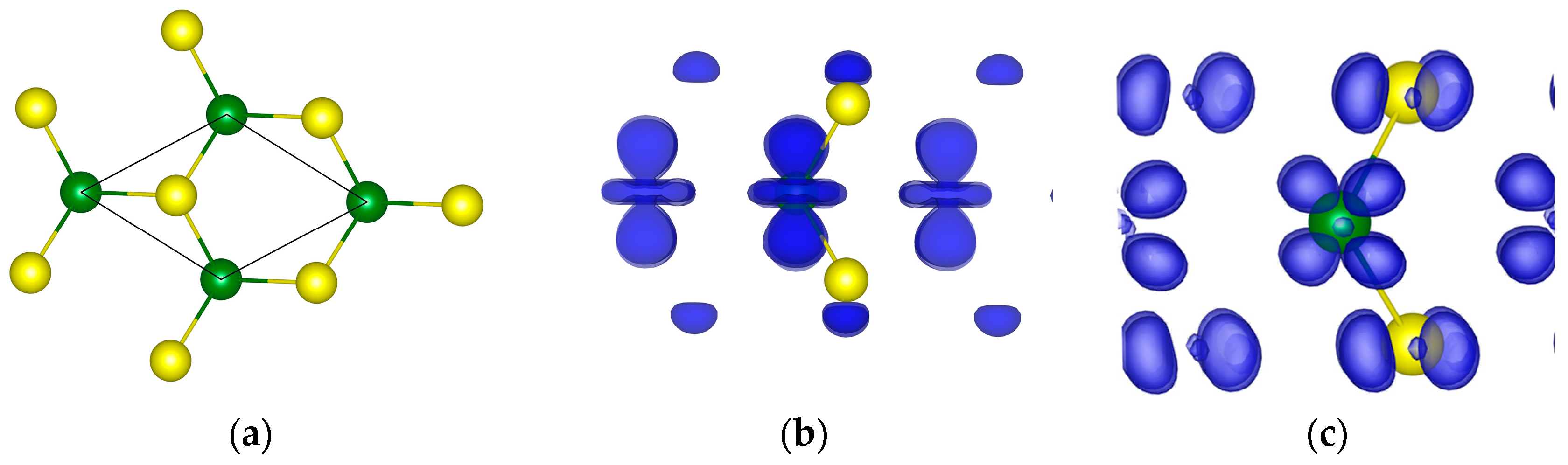
Figure 4.
The orbital DOS (a) and the band structure (b) of 1 L MoS2 obtained with PBE approximation. The electronic band gap is 1.8 eV.
Figure 4.
The orbital DOS (a) and the band structure (b) of 1 L MoS2 obtained with PBE approximation. The electronic band gap is 1.8 eV.


Table 1.
Excitonic energies (in meV) for different hole states in GaAs obtained with different XC kernels. Here and in Table 2, if not specified we use the following parameters for the local and LR kernels: . The experimental values for the exciton binding energies are 1.51–4.9 meV (the heavy-hole energy is larger, around 5 meV) [45,46].
| XC Kernel | (hh1) | (hh2) | (lh) |
|---|---|---|---|
| contact | −2.000 | −2.284 | −1.437 |
| Slater | −1.332 | −1.833 | −1.293 |
| LR | −0.492 | −0.511 | −0.442 |
| GEA | −0.183 | −0.221 | −0.224 |
| LDA | −0.216 | −0.270 | −0.308 |
| PBE | −0.250 | −0.323 | −0.447 |
| PW91 | −0.222 | −0.282 | −0.295 |
| PW corr | −0.0004 | −0.00067 | −0.001488 |
Table 2.
Excitonic energies (in eV) in 1L MoS2 obtained with different XC kernels. The experimental estimations for the excitonic binding energies are 0.2–0.5 eV [31,32].
| XC Kernel | Binding Energy, eV |
|---|---|
| local | −2.661 |
| local | −0.300 |
| Slater | −1.067 |
| LR | −0.106 |
| LR | −0.300 |
| GEA | −0.007 |
| LDA | −0.0096 |
| PBE | −0.0118 |
| PW91 | −0.0097 |
| PW corr. | −0.00001 |
© 2017 by the authors. Licensee MDPI, Basel, Switzerland. This article is an open access article distributed under the terms and conditions of the Creative Commons Attribution (CC BY) license (http://creativecommons.org/licenses/by/4.0/).
Share and Cite
MDPI and ACS Style
Turkowski, V.; Din, N.U.; Rahman, T.S. Time-Dependent Density-Functional Theory and Excitons in Bulk and Two-Dimensional Semiconductors. Computation 2017, 5, 39. https://doi.org/10.3390/computation5030039
AMA Style
Turkowski V, Din NU, Rahman TS. Time-Dependent Density-Functional Theory and Excitons in Bulk and Two-Dimensional Semiconductors. Computation. 2017; 5(3):39. https://doi.org/10.3390/computation5030039
Chicago/Turabian StyleTurkowski, Volodymyr, Naseem Ud Din, and Talat S. Rahman. 2017. "Time-Dependent Density-Functional Theory and Excitons in Bulk and Two-Dimensional Semiconductors" Computation 5, no. 3: 39. https://doi.org/10.3390/computation5030039
Note that from the first issue of 2016, this journal uses article numbers instead of page numbers. See further details here.