Performance Comparison of Feed-Forward Neural Networks Trained with Different Learning Algorithms for Recommender Systems

1
Software Engineering Lab, Graduate School of Computer Science and Engineering, University of Aizu, Aizuwakamatsu 965-8580, Japan
2
Department of Software Engineering, Bayero University Kano, Kano 700231, Nigera
*
Author to whom correspondence should be addressed.
†
These authors contributed equally to this work.
Computation 2017, 5(3), 40; https://doi.org/10.3390/computation5030040
Submission received: 6 August 2017
/
Revised: 4 September 2017
/
Accepted: 12 September 2017
/
Published: 13 September 2017
(This article belongs to the Section Computational Engineering)
Abstract
:Accuracy improvement is among the primary key research focuses in the area of recommender systems. Traditionally, recommender systems work on two sets of entities, Users and Items, to estimate a single rating that represents a user’s acceptance of an item. This technique was later extended to multi-criteria recommender systems that use an overall rating from multi-criteria ratings to estimate the degree of acceptance by users for items. The primary concern that is still open to the recommender systems community is to find suitable optimization algorithms that can explore the relationships between multiple ratings to compute an overall rating. One of the approaches for doing this is to assume that the overall rating as an aggregation of multiple criteria ratings. Given this assumption, this paper proposed using feed-forward neural networks to predict the overall rating. Five powerful training algorithms have been tested, and the results of their performance are analyzed and presented in this paper.
1. Introduction
Recommender systems are fast becoming essential instruments for both industries and academic institutions in addressing decision-making problems, such as choosing the most appropriate items from a large group of items. They play important roles in helping users to find items that might be relevant to what they want [1,2]. Nowadays, many definitions have been suggested for the term recommender system, but the most common one is to define it as an intelligent system that predicts and suggests items to the users that might match their choices. Another simple way to explain it is to assume there are two sets ( and ) consisting of the users of the system and the items that will be recommended to them respectively. A recommender system uses a utility function f to measure the likeness of an item i by a user u, where and . This relationship can be represented as: , where is a rating, which measures the degree to which the user may accept the item. Recommender systems seek to estimate for each relationship and recommends items with higher rating values to the users [3].
Several forms of supervised learning algorithms have been applied to predict users’ preferences of unseen items from a vast catalog of products using datasets of numerical preferences within some closed interval (e.g., 1 to 10). The most commonly used algorithms are content-based filtering, collaborative filtering, knowledge-based, and hybrid-based which combines two or more algorithms in different ways [4]. However, these kinds of the systems have some fundamental issues such as sparsity, cold start, and scalability problems. These problems have significantly affected the performance of the recommender systems. Artificial neural networks can be used to handle some of these problems as proposed by Zhao et al. [5], where contextual information are incorporated into the systems and modeled as a network of substitutable and complementary items. Another major drawback with these kinds of recommender systems is the of a single rating to decide whether the user is interested in the item or not. There is a considerable amount of research that establishes the limitations of single rating traditional recommender systems [6]. This is because there are many attributes of items used by users to decide on the usefulness of the items. Recent developments in the domain of recommender systems have heightened the need for considering some of these major attributes of items to make more accurate recommendations.
Multi-criteria recommender systems have invoked some of the most remarkable current discussions for solving some of the difficult problems of traditional recommendation systems. This area has been studied by many researchers [6,7], and it shows more reasonable recommendation accuracy over the traditional techniques. However, the central question is how to model the criteria ratings to estimate the overall rating that can be used in making the final recommendation. Consequently, Gediminas et al. [6] challenge the recommender systems community to use some of the sophisticated machine learning algorithms (especially artificial neural networks) to predict overall ratings based on the ratings given to the criteria. Even though a lot of research has been carried out on multi-criteria recommender systems, what is not yet clear is the impact of other sophisticated machine learning algorithms such as artificial neural networks in improving recommendation accuracy for multi-criteria recommendation problems. These challenges are currently quite open. This paper seeks to pursue this challenge by proposing different learning algorithms to train artificial neural networks using movie recommendation data sets. The aim of the study is to examine the emerging performance of some learning algorithms such as backpropagation (gradient descent-based), Levemberg-Marquardt, simulated annealing, Delta rule, and genetic algorithms in training artificial neural networks to shed more light on which option to pursue when using neural networks to improve the accuracy of multi-criteria recommender systems. This research will provide a significant opportunity to advance our understanding of the better algorithms to use for training neural networks, especially when modeling multi-criteria recommendation problems. The paper is composed of five themed sections, including this introduction section. Section 2 begins by laying the theoretical background of multi-criteria recommender systems, artificial neural networks, and the training algorithms used. Section 3 contains the details of the experiments conducted, while results and discussion of the study are provided in Section 4. Finally, the conclusion in Section 5 gives a summary of the work and identifies potential areas for future research.
2. Background
This study covers many independent research domains within the area of computational science. Therefore, at this point, it is considered necessary to give a brief panorama of the topics concerned. The most important areas to understand are the multi-criteria recommender systems and artificial neural networks, followed by the training algorithms.
2.1. Multi-Criteria Recommender Systems (MCRSs)
MCRSs were proposed principally to overcome some of the shortcomings of traditional recommendation techniques by taking into consideration the users’ preferences based on multiple characteristics of items to possibly provide more accurate recommendations [8]. This technique has been applied in many popular recommendation domains such as product recommendations [9], tourism and travel domains[10], restaurant recommendation problems [11], research paper recommendations [12], e-learning [13] and many others.
The MCRSs technique extends traditional recommender systems by allowing the users to give ratings to several items’ characteristics known as criteria. Each criteria rating for , provides additional information about users’ opinions on the items; for instance, in a movie recommendation problem, users may like a movie based on action, story, visuals, or the direction of the movie. Therefore, users are expected to give ratings for those criteria and possibly with an additional rating called the overall rating. Hence, the utility function of traditional recommender systems introduced briefly in the introduction section needs to be extended to account for multiple criteria ratings as presented in (1) below:
Because of the nature of the utility function (see (1)), it becomes necessary to introduce a new technique that can use all the ratings for making more accurate predictions. There are two main approaches used for calculating user preferences in MCRSs. One of them is the heuristic-based approach that uses multidimensional similarity metrics to calculate similarity values on each criterion together with the overall rating , and the second one is the model-based approach in which a model is built to estimate the . An aggregation function model is a perfect example of the model-based approach that computes as a function of other criteria (see (2)).
2.2. Artificial Neural Networks (ANNs)
ANNs are coordinative intelligent systems consisting of neurons as the essential elements. They are powerful algorithms initially inspired by the goal of implementing machines that can imitate the human brain [14]. ANNs strive to simulate, in a great fashion, the network of neurons (nerve cells) of the biological nervous system. The physical structure and information processing of the human brain are partially imitated with collections of interconnected neurons to model nonlinear systems [15]. Neurons are cells in the brain that contain input wires to other neurons called dendrites and output wires from a neuron to other neurons called axons.
Neurons are computational units that accept inputs via dendrites and sends the result to another neuron after the computations through the axon. Neurons are organized in ANNs in the form of layers. A layer that receives inputs from the external environment is called an input layer and the one that presents the computational results is referred to as the output layer. Between the input and output layers, there may be other layers called hidden layers. Every neuron in the network belongs to exactly one layer, and there may be several neurons in one layer. ANNs architecture is referred to as a feedforward network if the flow of signal is in a direction in which the input values are fed directly into the input layer, then to the next layer after the computation. ANNs that contain at least three layers (input, output, and one or more hidden layers) are called multi-layer ANNs (or MANNs for short). The underlying architecture of MANNs is given in Figure 1, containing one hidden layer. ANNs are fully connected, which means that each neuron at every layer is attached to all neurons in the adjacent layer [16].
The output of ANNs is a computational result of an activation function where is a vector of synaptic weights between neurons and is a vector of the input values. contains important parameters that the ANNs need to learn for determining an accurate output value for any input values in . The can be of different types such as a sigmoid (logistic) activation function (), linear activation function (), tangent hyperbolic activation function (), etc. In working with the ANNs, an appropriate activation function must be defined at each layer that receives signals from the previous layer to scale the data output from the layer. The choice of the kind of activation function to use depends on the nature of the output the neuron is expected to provide.
However, as the output of the network depends on the synaptic weights and bias, the central question in using ANNs to solve any machine learning problem is to think about how the networks will be trained in learning the appropriate connection weights to produce optimal outputs. The target is to find a value that can be used to update the weights based on some given criteria. Several algorithms can be used to find to train ANNs. In the subsequent sections, we briefly explain some of the possible algorithms for training ANNs.
2.3. Delta Rule Algorithm (DRA)
The DRA is a popular and efficient algorithm for training ANNs that does not contain hidden layers. It is based on a gradient descent algorithm that was developed to train two-layer networks which deal with a nonlinearly separable data set. It uses a constant learning rate , which is a parameter that controls how much the updating steps can affect the current values of the weights. It also contains the derivative of the activation functions , the error between real and estimated outputs, and the current features to compute (see (3), is the actual value from the data set) so that the updated weights that can be used in the iteration will be computed using (see (4)). Note that in this experiment, the DRA algorithm may be referred to as ADAptive Linear Neuron (Adaline) algorithm.
2.4. Backpropagation Algorithm (BPA)
Section 2.2 explained the basic architecture of MANNs, and how features are forward propagated from the input to the output layer. Although the algorithm described in Section 2.3 works quite well for ANNs having only two layers, this algorithm can not be applied to ANNs with more than two layers. To solve this problem, BPA is one of the algorithms used to determine the optimal values of weights in MANNs. There are two versions of back-propagation algorithms employed in this experiment: the gradient descent-based, and Levenberg-Marquardt-based BPA. For simplicity, this study refers to gradient descent-based algorithm simply as “BPA” (discussed here) and the Levenberg-Marquardt algorithm-based as “LMA”. BPA works by training the networks to produce the estimated output . As each feature set is presented to the network, errors are calculated between the outputs of the networks for feature sets. The weights’ matrix is then modified to minimize the errors. In an experiment with training data containing N features, the average error is determined as follows:
The following steps explained how BPA works according to some of the recent implementations of the algorithm [17].
- Define the training sets and randomly generate the synaptic weights.
- Advance the training data set from the input to the output layer via the hidden layers to obtain the estimated output.
- Calculate the error using (5).
- Terminate the training if the error satisfies the given criteria or if the maximum number of iteration is reached.
- Update the synaptic weights of the networks according to the layers.
- Go to step 2.
Calculating using BPA is a bit lengthy compared to doing so with Adaline. It requires someone to have a basic mathematical background, especially the rules of differential calculus. We therefore skip the derivation, but the reader can find a detailed explanation of this derivation in [16].
2.5. Levenberg-Marquardt Algorithm (LMA)
LMA was proven to be among the most efficient optimization algorithms for solving various minimization problems than conjugate gradient techniques like the dog-leg algorithm, the double dog-leg algorithm, the truncated conjugate gradient, two-dimensional search methods, as well as the gradient descent algorithm [18]. It is used to solve nonlinear least square optimization problems that look exactly like the error function in (5).
To highlight how the LMA computes the error function and updates the weights, let ; we can rewrite the error function over the feature set x as where x contains the elements . is a function which is an error for feature set where . To put it in a simpler form, we can take the error function E as a vector of errors defined by so that the error E can be written as . Let’s define a Jacobian matrix as a matrix of the derivatives of the error function with respect to x as for and . The weight update can be obtained using (6), and for the new weights, we go back to (4).
2.6. Genetic Algorithm (GA)
GA is a very prominent non-traditional optimization technique which resembles the theory of evolution. It is an adaptive search algorithm that works based on the methods of natural selection. Unlike the previous algorithms, GA works based on logic, not derivatives of a function and it can search for a population of solutions, not only one solution set. The logic it uses is based on the concept of ‘Survival of the fittest’ from Darwin’s theory [19] which means only the most competent individual will survive and generate other individuals that might perform better than the current generation.
While a variety of explanations can be found about this algorithm in the literature, the most common way to explain GA is to look at it as a replica of biological chromosomes and genes, where the chromosome is a solution set or an individual containing the set of parameters to be optimized, and a gene represents single components of those parameters. New generations of chromosomes can be generated by manipulating the genes in the chromosomes. A collection of chromosomes is known as a population, and the population size is the exact number of chromosomes in the experiment. Two basic genetic operators ‘mutation’ and ‘crossover’ are used to manipulate genes in the chromosomes.
The crossover operation combines genes from two parents to form an offspring, while the mutation operation is used to bring new genetic material into the population by interchanging the genes in the chromosome [20]. The following steps summarize how GA works in solving optimization problems.
- Generate n population of chromosomes at random.
- Compute the fitness ( in our case) of each chromosome.
- Generate a new population using the selected GA operator.
- Run the algorithm using the newly generated population.
- Stop if a particular stopping condition is satisfied or
- Go back to step 2.
Chromosomes are selected as parents for step (3) based on some selected rule (GA operator) to produce new chromosomes for the next iteration. In this experiment, the stochastic universal sampling technique was adopted. This method chooses potential chromosomes according to their calculated fitness value in step (2) [15]. Both mutation and crossover were applied concurrently to reproduce the fittest offspring.
2.7. Simulated Annealing Algorithm (SMA)
The SMA is a non-traditional optimization algorithm that uses some probabilistic laws to search for an optimal solution. In science and engineering, the word ‘annealing’ is defined as a thermal method of getting low energy states of a solid in a heat bath by initially changing the temperature of the heat bath to the melting state of the solid and then lowering it down gently for the particles to organize themselves as in the initial state of the solid [21]. The SMA mimics the adaptive metropolis algorithm [22], which is a procedure used for sampling a specified distribution of a large data set. In 1953, Metropolis et al. [23] introduced an algorithm based on Monte Carlo methods [24] to simulate the change of states of a solid in a heat bath to thermal equilibrium in the following way. Let be the energy of the solid at a state i, any subsequent energy of the same solid at state j can be generated by transforming using a perturbation mechanism. If the difference , then will be accepted directly, otherwise, will be accepted with a certain probability , where the parameter c is called a Boltzmann constant and T is the temperature of the heat bath. Similarly, the SMA generates sequence of solutions to optimization problems by replacing a state in the Metropolis algorithm to serve as one solution, and the energy of the state as a result produced by the activation/error function E. Therefore, if we have two solutions and , then the values produced by functions can be written as and respectively. Accepting to replace depends on the probability distribution given in (7), where k is a real number called a control parameter (similar to the Boltzmann constant, c). This result can be generalized to any two solutions and for .
Updating the weights in SMA-based networks requires a vector of step lengths of the weights matrix W, with and . The error produced by W is calculated in a manner similar to (5), and the subsequent weights can be computed by changing the individual weight (see (8)). r is a random number between −1 and 1.
2.8. Randomized and Ensemble Methods
Another training approaches that even though have not been experimented in this study are the randomized and ensemble approaches. We briefly mention them here to serve as additional guides to someone who might be interested in improving the accuracy of the approaches we analyzed. Similar to SMA and GA, both randomized and ensemble methods are optimization techniques that have been studied extensively for improving the performance of ANNs. A Random Neural Networks (RNN) was introduced in the inaugural RNN paper [25], which has found to be capable of providing excellent performance in various areas of application [26] and has motivated many theoretical papers [27]. A recent survey of randomized algorithms for training neural networks conducted by [14] provides an extensive review of the use of randomization in kernel machines and related fields. Furthermore, Ye et al. [28] provide a systematic review and the state-of-the-art of the ensemble methods that can serve as a guideline for beginners and practitioners. They discussed the main theories associated with the ensemble classification and regression. The survey reviewed the traditional ensemble methods together with the recent improvements made to the traditional methods. Additionally, the survey outlined the applications of the ensemble methods and the potential areas for future research.
3. Experimental Section
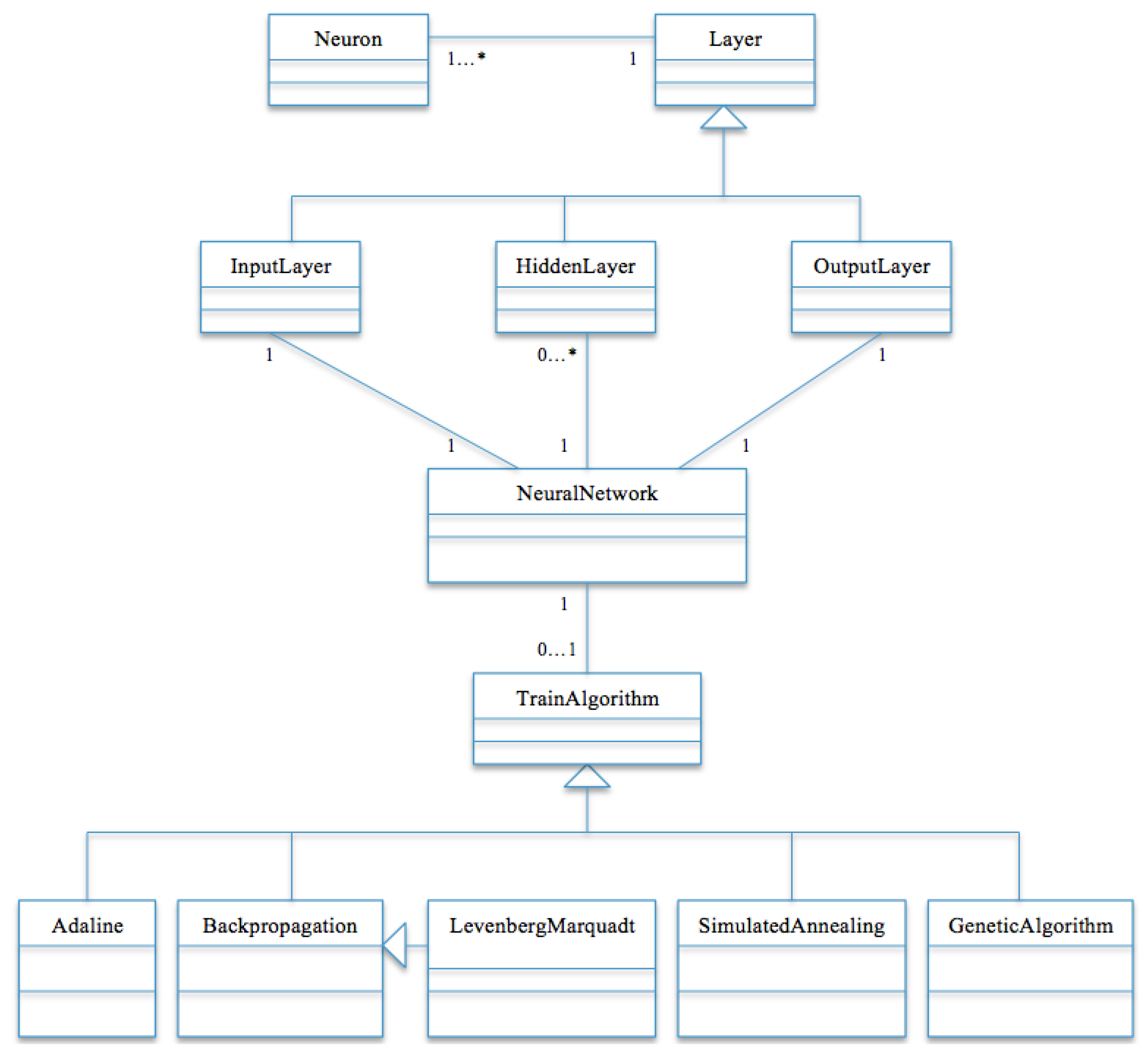
The experiment was carried out by using object oriented programming techniques with Java [29] to develop the ANNs [17] and to use five training algorithms to train the models. The skeleton of the class diagram implemented for carrying out the study is shown in Figure 2. Note that the diagram did not constitute all the classes used in the experiment; for instance, the genetic algorithm alone contains additional classes such as the chromosomes class, individual class, and so on. Lee et al. [30] gave a straightforward explanation of the classes required to implement genetic algorithms in Java. Nevertheless, the figure just gives an abstract architecture of the model. Additionally, the simulation of the five algorithms is undertaken using a Windows personal computer (NCC, Abuja, Nigeria) with system configuration as Intel® Core™ i7-3612QM CPU @2.10 GHz 2.10 GHz and installed memory (RAM) of 4.00 GB.
Furthermore, in all five experiments, the weights of the neural network were randomly generated to form a matrix of weights as arrays of floating point numbers between some given interval (mostly between 0 and 1. Sometimes the range is determined by values of other variables like the starting temperature as in the case of simulated annealing). Two or more weights can have the same real value since weights of neural networks are independent of one another. The progress of the five algorithms was monitored based on the series of training cycles.
Moreover, analogous to the case of the SMA, GA also requires some parameters for the algorithm to work efficiently. The population of the candidate solution was first randomly generated to begin the training. Individuals in the population known as chromosomes contain floating point numbers called genes. The number of chromosomes to participate in the training needs to be specified. Also, the experiment requires a parameter that determines the percentage of chromosomes to mate based on the fitness values and reproduced offspring that will be used for future iterations. Mating in this context means pairing of two chromosomes to exchange some of their genes to generate new chromosomes that are expected to have higher fitness than the parents. The experiment requires the percentage of the number of genes that two pairs of chromosomes can exchange randomly as a parameter. Several values of those parameters were tested to choose an optimal solution.
On the other hand, the remaining three algorithms (Adeline, BPA, and LMA) share many things in common. Their basic requirements are to define activation functions at each layer of the network (except at the input layer), and also to set the learning rate to a real number to control the speeds of which the networks produced optimal solutions. Different values have been tested to prevent the networks from oscillating between solutions, or to prevent the networks from diverging completely, or to prevent longer convergence time. In the same manner, as in the previous algorithms, the number of training cycles and the target error value were also specified. The activation functions used are the linear activation function for the output layers and the sigmoid logistic function for the hidden layers in BPA and LMA. Each of the four MANNs consists of three layers: input, hidden and output layers (see Figure 1), with five neurons in the input layer.
Moreover, a data set extracted from Yahoo!Movies [31] was used in the experiments. It consists of multi-criteria ratings obtained from users who rate movies based on four different characteristics. The criteria ratings are considered as to determine the preferences of users on movies. The criteria ratings are for the action, the story, the direction and the visual effects of the movies, represented by , , , and respectively. The ratings were measured using a 13-fold quantifiable scale from to F representing the highest and the lowest references for each criterion , for as in Table 1, where is the overall rating.
To obtain numerical ratings that can be suitable for the experiments, the ratings in Table 1 were transformed to numerical ratings (see Table 2). The most preferred rating () is represented by an integer number 13, and the least preferred rating (F) is replaced by 1. The same changes have been made to all other ratings ().
Data cleaning was performed after the transformation to remove cases that have missing ratings either among the four criteria or the overall rating. Likewise, movies rated by few users were taken out of the experimental data. The resulting data set used for the study contains approximately 62,000 ratings from 6078 users to about 1000 different movies.
Furthermore, when training ANNs, for various reasons such as the type of activation function used, it is important to perform other preliminary treatments on the data set before the training [32]. For instance, when using a logistic sigmoid function as the activation function of the neurons, which produces an output between 0 and 1, then the interval of the output values from the activation function has to be respected. Although data normalization has been used by many researchers and shows significant improvements in the results and reduction of the length of the training period, no particular method is recommended for data normalization. However, the most important thing is to normalize the data with respect to the range of values given by the candidate activation function [32,33]. For this reason, we considered taking the ratio between each entry in the data set to the maximum number of all the entries. Recall that all the entries in Table 2 are between 1 and 13, then dividing each by 13 gives the desired result in a normalized form . For example, the first row of Table 2 will be in the form for the action, the story, the direction, the visuals, and the overall ratings respectively.
We used statistical data analysis techniques to compute the linear relationships between the criteria ratings and the overall rating, and also to find the statistical significance of each criteria rating with respect to the overall rating. The Pearson correlation coefficient was used for computing the linear relationships while the significance was obtained using P-Value by setting the significance level to 5% (). Table 3 displays the results which indicate that all the correlations are statistically significant.
Additionally, the experiment was conducted, and the results were analyzed using two types of data sets: the training and testing set. The two sets are in the ratio of 3:1 (75% and 25% ) of the entire data set for training and testing respectively.
3.1. Parameter Settings
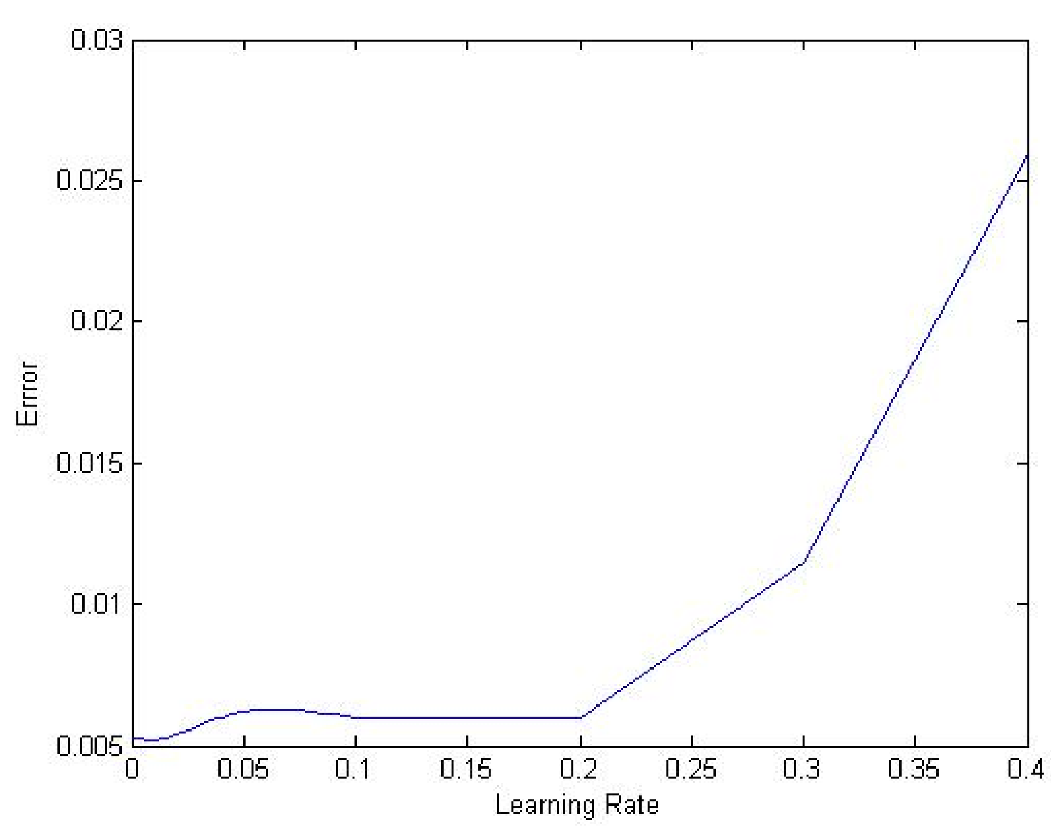
The first step necessary to achieve an accurate performance of the algorithms was to select appropriate parameter values required by each algorithm. Consequently, the experiment started by choosing a constant positive number between 0 and 1 to serve as the learning rate. Several values were tested to find the one that provided the minimum MSE and also allowed the networks to converge. Therefore, we started with a relatively high value (0.4) and monitored the performance of the algorithms. The same process was repeated many times by decreasing the value as the training continued. Figure 3 shows the errors for different learning rates. We decided to choose 0.01 as a good value for the experiments. The same procedure was followed to choose the population size, the mutation rate, and the starting temperature for the genetic and simulated annealing algorithms respectively. We considered relevant literature and used comparable methods of selecting the experimental parameters [34] and taking various precautions to avoid premature convergence [35]. The target training error used in all the experiments was set to . In SMA, setting the T was done carefully to ensure that the initial probability of accepting the solutions be close to 1. However, too high T may result in bad performance and long training computation time. According to Bellio et al. [36] choosing T in the interval [1, 40] and was confirmed to provide better performance of the SMA. Therefore we initialized , and Q was generated randomly within the above interval. Furthermore, to prevent accepting bad solutions, the minimum value that T can take was set to 1, and the was epoch 500 iterations. The stopping condition depends on attaining the target error, , or the number of iteration equals 500.
Similarly, in the GA experiment, the elitism number was set to 5, epoch to 100 iterations, and population size to 100 chromosomes. Other relevant parameters are the mutation and crossover probabilities. After conducting a sensitivity analysis, we select the crossover probability to be 85%, and the mutation probability to 9%. The stopping condition depends on the epoch and the target error.
4. Results and Discussion
Mean square error (MSE) was proposed as the criteria for evaluating the performance of the learning algorithms during training and testing phases of the study. It was used to measure how close the outputs of the networks were to the real values from the data set. It was explained in Section 2.4 when discussing (5), which for every output, the MSE takes the vertical distance between the actual output and the corresponding real value and squares the value. Then for each iteration, it adds up all the values and divides by the number of the input sets from the data set. This metric was chosen due to its non-negative characteristics and suitable statistical properties.
Furthermore, the result of the experiment for comparing the effectiveness of the algorithms is shown in Table 4. It contains the total number of iterations required by the algorithms for training, the training and test errors, the correlation between the estimated and actual outputs in the test data set, as well as the p-value which is a function that measures how close the predicted outputs are relative to the actual values. Moreover, the correlation coefficients between the actual outputs of the five experiments and the real values are presented in Table 5.
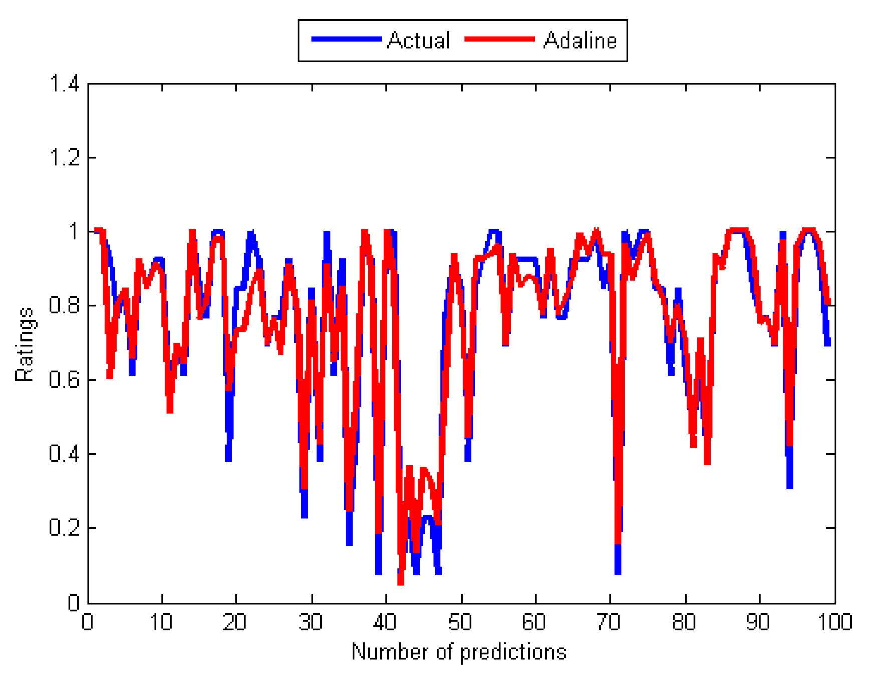
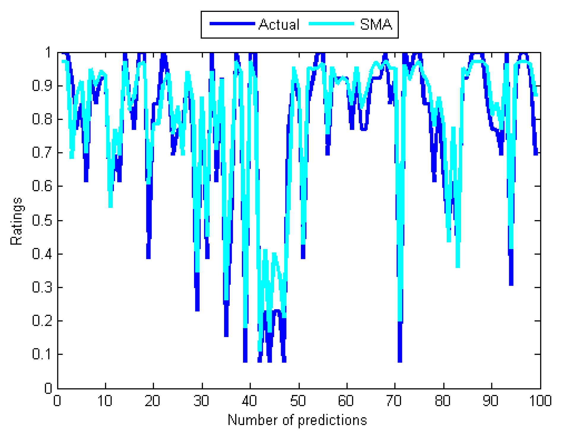
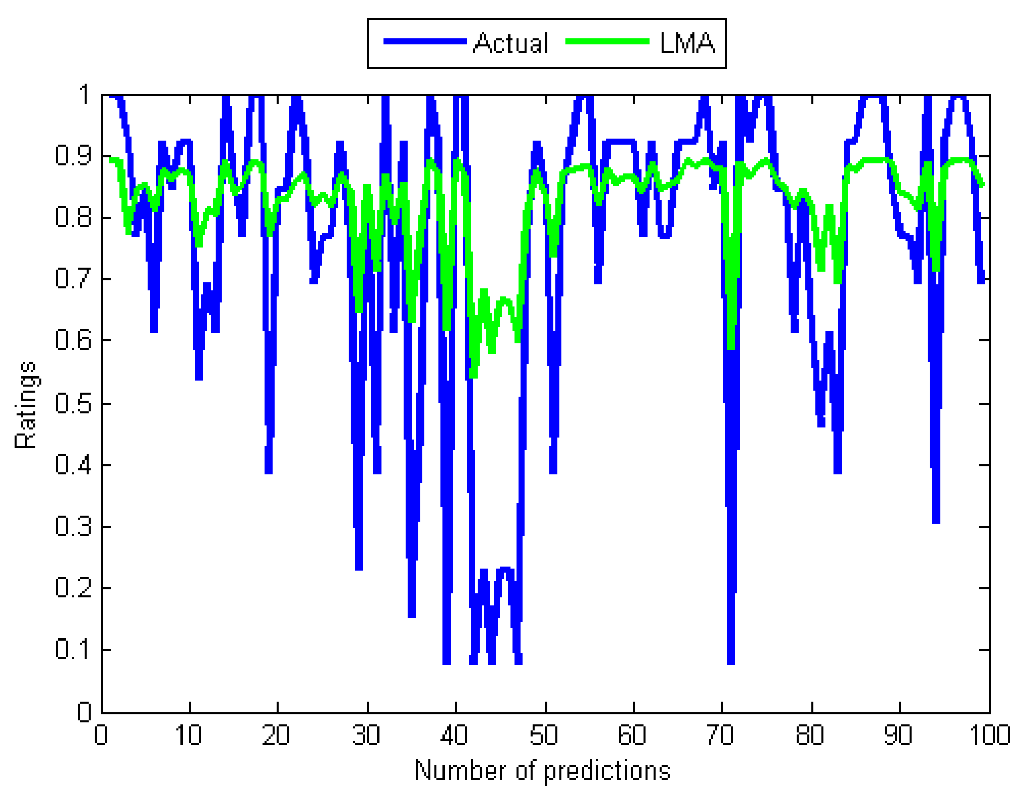
The results in Table 4 and Table 5 are supported by graphs in Figure 4, Figure 5, Figure 6, Figure 7, Figure 8 and Figure 9 that show the relationships between the actual values (see Figure 4) and those of the five algorithms in Figure 6, while Figure 5, Figure 6, Figure 7, Figure 8 and Figure 9 contain pairs of curves of the actual values and the output of the individual training algorithm. The findings show the advantages and disadvantages of the five algorithms used, in particular between the ones used for training the MANNs. The rest of this section discusses the findings of the study. Subsequently, some issues that determined the predictive performance of the five networks were identified. The explanation begins by first considering the architectural differences between the networks regarding the differences in accuracy of the four algorithms used to train the MANNs. To begin with, it is interesting to note that among the two architectures (single and MANNs) and five algorithms employed in this study, the Adaline network performs better than the MANNs trained with any of the other four algorithms. According to Table 4, the MSE of Adaline was observed to be better than MANNs training algorithms, which also confirmed the efficiency of single layer networks [37], and consequently, it is not necessary to implement MANNs trained with any of the remaining algorithms for improving the prediction accuracy of MCRSs. This observation is consistent with the result shown in Table 5 and Figure 5 and Figure 6 that showed that the neural network trained using Adeline has the strongest linear relationships with the actual values from the test data. Another strong piece of evidence of the efficiency of the Adaline network is the computation speed and the number of training cycles required for the algorithm to converge. This can be seen from the second column in Table 4 where it was reported that Adaline requires significantly fewer iterations than the other four algorithms.
However, the performances of the training algorithms for MANNs are not all that bad. Together, these results provide significant insights into choosing the appropriate algorithm for training MANNs. Although the LMA and BPA have high computation speeds compared to the GA and the SMA, the study reveals that BPA and LMA have slow convergence rates. By comparing the five results, it can be seen that the convergence of the BPA is extremely slow. Moreover, the training and test errors of the two back-propagation algorithms are the highest. This became apparent after performing several computations of the derivatives of the error functions that can make their outputs to be maximally wrong since strong errors for adjusting the weights during the training can not be produced. In respect to this, the graphs of their predicted values in Figure 7 and Figure 8 did not show reasonable correlations with the actual values from the data set. A comparison of the two results reports that the LMA outperforms and achieves faster convergence than the BPA. Another problem of back-propagation algorithms that may contribute to their poor performance is their inability to provide global solutions since they can get stuck in local minima. On the other hand, the GA and the SMA have the potential to produce global search of neurons’ weights by avoiding local minima.
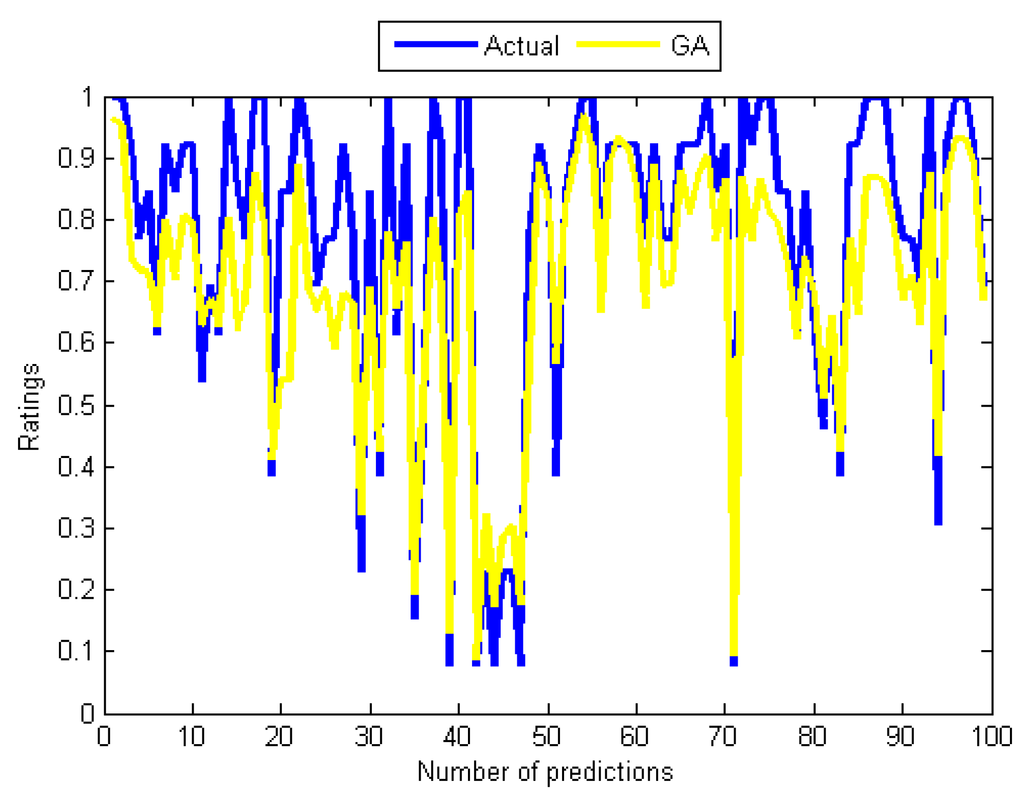
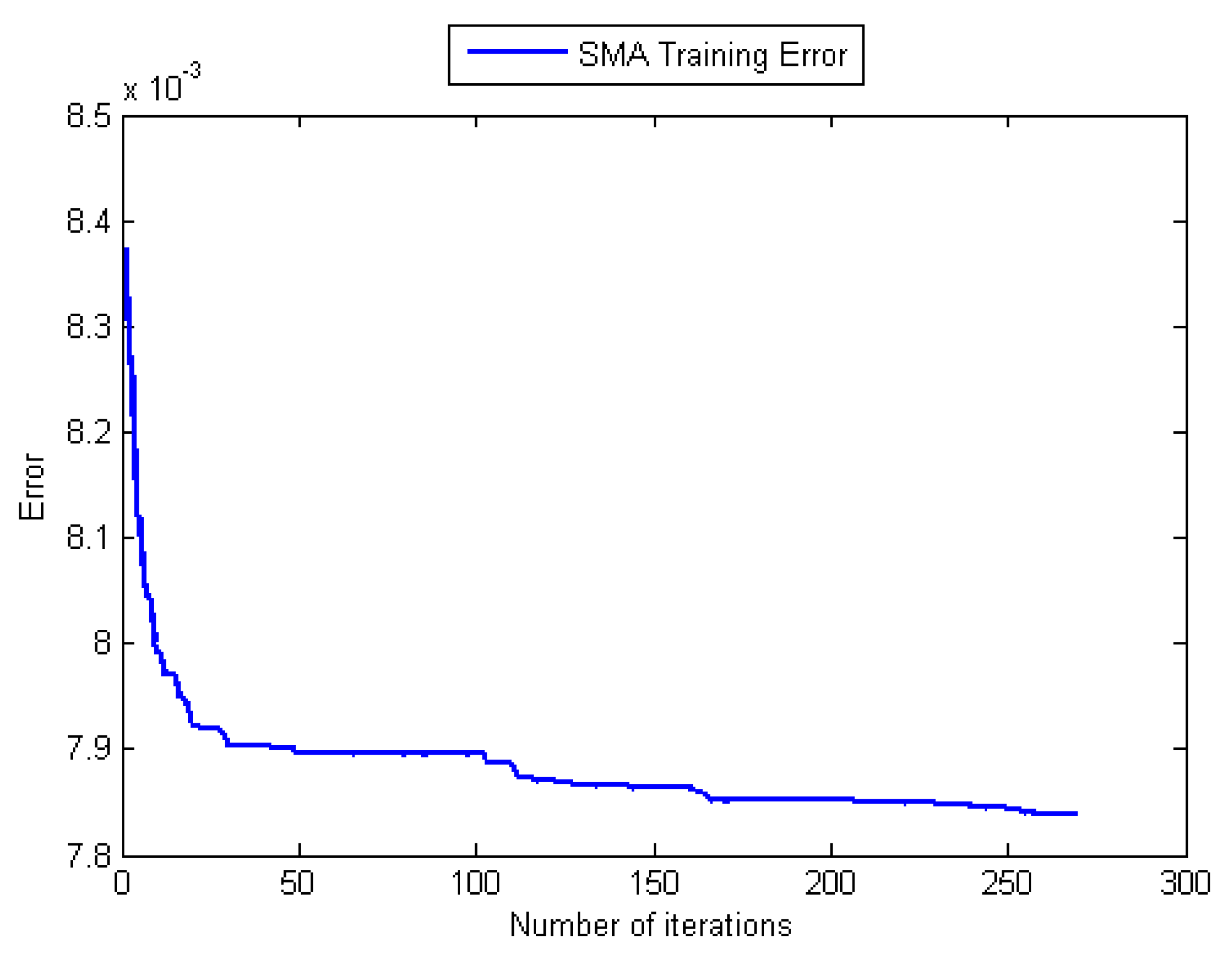
Although the GA does not require many training cycles (see Table 4), its outstanding problem is long computation time which is related to the population size and several operations like evaluating fitness and sorting the population based on fitness. Turning also now to the experimental evidence, the results in Table 4 and Table 5, and that of Figure 6 and Figure 9 indicate that the GA-based network has outperformed the two back-propagation algorithms. In the final part of the discussion, the single most striking observation to emerge from the data comparison was the ability of the SMA-based network to provide better prediction than all the remaining three MANNs. The performance of the SMA is close to that of Adaline except for the number of training cycles, which was higher compared to Adaline and the GA. However, when using the SMA, it is important to bear in mind that the error performance curve during training was not completely smooth unlike the case of the BPA and the LMA, which means that the same error value could be repeated many times before convergence. This is illustrated in Figure 11, which is the error versus the number of iterations (epoch) curve that shows the nature of its performance during the training. Overall, it can be seen from Table 4 and Figure 5, Figure 6 and Figure 11 that Adaline and SMA-based models have the lowest MSE values and provide more accurate estimations of the target values. Their performance on training and test data indicates that the two models have good predictive potentials.
Finally, as both BPA and Adaline used partial derivatives to update the weights (see (3) for example), the results indicate that additional hidden layer increases the number of iterations and the test errors, proving that the simple network is enough to estimate the overall rating in multi-criteria recommendation problems, and hence more complex network that contains hidden layers is not required.
5. Conclusions and Future Work
Recently, Adomavicius et al. [6,38] challenged the recommender systems research community to use artificial neural networks in modeling MCRSs for improving the prediction accuracy while predicting the overall rating. Based on our knowledge, up to the present, no one has attempted to pursue this challenge. This paper presented a comprehensive comparison between the experimental results of five different neural network models trained with five machine learning algorithms.
This study aimed at addressing the problems of choosing an optimal neural networks architecture and efficient training algorithms to train the networks for modeling the criteria ratings to compute an overall rating in MCRSs using an aggregation function approach. Two types of neural network models were designed and implemented, one of them consisting of only the input and output layers and the other four models containing hidden layers. The study used five different powerful training algorithms to train the networks. The advantages and disadvantages of each algorithm regarding prediction accuracy, the length of training time, and the number of iterations required for the networks to converge were investigated and analyzed. This experiment produced results which support the findings of a large amount of some of the previous work in the field of computational intelligence.
The study makes significant contributions not only to the recommender system research community but also to other industrial and academic research domains that are willing to use neural networks in solving optimization problems. The results of the experiment can serve as recommendations and guidelines to the reader when choosing a better architecture and suitable training algorithms for building and training neural network models.
The research findings admit several future research topics that need to be taken to investigate other possibilities of improving the prediction accuracy of MCRSs. For instance, the study shows that some of the algorithms are more efficient than othersregarding prediction accuracy, speed, the number of training iterations, and so on. Future research work needs to investigate the possibility of improving the accuracy through hybridization of two or more algorithms. For instance, a hybrid between the BPA and the LMA might improve the faster convergence ability, and with the SMA or the GA approach could improve the searching capacity and avoidance of getting trapped at local optima. Köker and Çakar [39] observed that hybrids with those algorithms could reduce the number of iterations, minimize the error, ease the difficulty in choosing parameters, and might produce a better result. More information on their performance using other evaluation metrics would help us to establish a greater degree of accuracy on this matter.
As the research was conducted with only one data set, future studies on the current topic that could use additional multi-criteria data sets to extend our understanding of the kind of architecture and the training algorithm that are suitable for modeling the criteria ratings are therefore recommended. Moreover, we suggest future studies on the current topic that would consider randomized algorithms and ensemble methods.
Acknowledgments
The authors would like to offer special thanks to the Editors of the Journal of Computational Engineering and the anonymous reviewers for their useful comments and recommendations, which helped significantly in improving the quality of this article.
Author Contributions
The experiments and writing the first version of the paper were done by Mohammed Hassan under the supervision of Mohamed Hamada. Hamada also proposed the structure of the paper and helped in proofreading and improving the quality of the article.
Conflicts of Interest
The authors declare no conflict of interest.
References
- Zhang, D.; Simoff, S.; Aciar, S.; Debenham, J. A multi agent recommender system that utilises consumer reviews in its recommendations. Int. J. Intell. Inf. Database Syst. 2008, 2, 69–81. [Google Scholar] [CrossRef]
- Hassan, M.; Hamada, M. A Framework for Recommending Learning Peers to Support Collaborative Learning on Social Networks. Int. J. Simul. Syst. Sci. Technol. 2016, 17. [Google Scholar]
- Hassan, M.; Hamada, M. Performance Comparison of Featured Neural Network Trained with Backpropagation and Delta Rule Techniques for Movie Rating Prediction in Multi-Criteria Recommender Systems. Informatica 2016, 40, 409. [Google Scholar]
- Hassan, M.; Hamada, M. Recommending Learning Peers for Collaborative Learning Through Social Network Sites. In Proceedings of the 7th International Conference on Intelligent Systems, Modelling and Simulation (ISMS), Bangkok, Thailand, 25–27 January 2016; pp. 60–63. [Google Scholar]
- Zhao, T.; McAuley, J.; Li, M.; King, I. Improving recommendation accuracy using networks of substitutable and complementary products. In Proceedings of the International Joint Conference on Neural Networks (IJCNN), Anchorage, AK, USA, 14–19 May 2017; pp. 3649–3655. [Google Scholar]
- Adomavicius, G.; Manouselis, N.; Kwon, Y. Multi-criteria recommender systems. In Recommender Systems Handbook, 2nd ed.; Springer: New York, NY, USA, 2015; pp. 854–887. [Google Scholar]
- Hassan, M.; Hamada, M. Enhancing learning objects recommendation using multi-criteria recommender systems. In Proceedings of the International Conference on Teaching, and Learning for Engineering (TALE2016), Bangkok, Thailand, 7–9 December 2016; pp. 62–64. [Google Scholar]
- Hassan, M.; Hamada, M. A Neural Networks Approach for Improving the Accuracy of Multi-Criteria Recommender Systems. Appl. Sci. 2017, 7, 868. [Google Scholar] [CrossRef]
- Palanivel, K.; Sivakumar, R. A study on collaborative recommender system using fuzzy-multicriteria approaches. Int. J. Bus. Inf. Syst. 2011, 7, 419–439. [Google Scholar] [CrossRef]
- Jannach, D.; Gedikli, F.; Karakaya, Z.; Juwig, O. Recommending Hotels Based on Multi-Dimensional Customer Ratings. In Information and Communication Technologies in Tourism 2012; Springer: Vienna, Austria, 2012; pp. 320–331. [Google Scholar]
- Sanchez-Vilas, F.; Ismoilov, J.; Lousame, F.P.; Sanchez, E.; Lama, M. Applying multicriteria algorithms to restaurant recommendation. In Proceedings of the 2011 IEEE/WIC/ACM International Conferences on Web Intelligence and Intelligent Agent Technology, Lyon, France, 22–27 August 2011; pp. 87–91. [Google Scholar]
- Zarrinkalam, F.; Kahani, M. A multi-criteria hybrid citation recommendation system based on linked data. In Proceedings of the 2nd International eConference on Computer and Knowledge Engineering (ICCKE), Mashhad, Iran, 18–19 October 2012; pp. 283–288. [Google Scholar]
- Weng, M.M.; Hung, J.C.; Weng, J.D.; Shih, T.K. The recommendation mechanism for social learning environment. Int. J. Comput. Sci. Eng. 2016, 13, 246–257. [Google Scholar] [CrossRef]
- Zhang, L.; Suganthan, P.N. A survey of randomized algorithms for training neural networks. Inf. Sci. 2016, 364, 146–155. [Google Scholar] [CrossRef]
- Göçken, M.; Özçalıcı, M.; Boru, A.; Dosdoğru, A.T. Integrating metaheuristics and Artificial Neural Networks for improved stock price prediction. Expert Syst. Appl. 2016, 44, 320–331. [Google Scholar] [CrossRef]
- Haykin, S.S.; Haykin, S.S.; Haykin, S.S.; Haykin, S.S. Neural Networks and Learning Machines, 3rd ed.; Pearson: Upper Saddle River, NJ, USA, 2009. [Google Scholar]
- Souza, A.M.; Soares, F.M. Neural Network Programming with Java; Packt Publishing Ltd: Birmingham, UK, 2016. [Google Scholar]
- Ranganathan, A. The levenberg-marquardt algorithm. Tutor. LM Algorithm 2004, 11, 101–110. [Google Scholar]
- Michalewicz, Z. GAs: What are they? In Genetic Algorithms+ Data Structures= Evolution Programs; Springer: Berlin/Heidelberg, Germany, 1994; pp. 13–30. [Google Scholar]
- Heaton, J. Introduction to Neural Networks with Java, 2nd ed.; Heaton Research, Inc.: St. Louis, MO, USA, 2008. [Google Scholar]
- Aarts, E.; Korst, J. Simulated Annealing and Boltzmann machines: A Stochastic Approach to Combinatorial Optimization and Neural Computing; John Wiley: Hoboken, NJ, USA, 1990. [Google Scholar]
- Beichl, I.; Sullivan, F. The metropolis algorithm. Comput. Sci. Eng. 2000, 2, 65–69. [Google Scholar] [CrossRef]
- Metropolis, N.; Rosenbluth, A.W.; Rosenbluth, M.N.; Teller, A.H.; Teller, E. Equation of state calculations by fast computing machines. J. Chem. Phys. 1953, 21, 1087–1092. [Google Scholar] [CrossRef]
- Gilks, W.R. Markov Chain Monte Carlo; Wiley Online Library: Hoboken, NJ, USA, 2005. [Google Scholar]
- Gelenbe, E. Random neural networks with negative and positive signals and product form solution. Neural Comput. 1989, 1, 502–510. [Google Scholar] [CrossRef]
- Igelnik, B.; Pao, Y.H. Stochastic choice of basis functions in adaptive function approximation and the functional-link net. IEEE Trans. Neural Netw. 1995, 6, 1320–1329. [Google Scholar] [CrossRef] [PubMed]
- Georgiopoulos, M.; Li, C.; Kocak, T. Learning in the feed-forward random neural network: A critical review. Perform. Eval. 2011, 68, 361–384. [Google Scholar] [CrossRef]
- Ren, Y.; Zhang, L.; Suganthan, P.N. Ensemble classification and regression-recent developments, applications and future directions. IEEE Comput. Intell. Mag. 2016, 11, 41–53. [Google Scholar] [CrossRef]
- Kendal, S. Object Oriented Programming Using Java; Bookboon: Copenhagen, Denmark, 2009. [Google Scholar]
- Jacobson, L.; Kanber, B. Genetic Algorithms in Java Basics; Springer: New York, NY, USA, 2015. [Google Scholar]
- Lakiotaki, K.; Matsatsinis, N.F.; Tsoukias, A. Multicriteria user modeling in recommender systems. IEEE Intell. Syst. 2011, 26, 64–76. [Google Scholar] [CrossRef]
- Sola, J.; Sevilla, J. Importance of input data normalization for the application of neural networks to complex industrial problems. IEEE Trans. Nucl. Sci. 1997, 44, 1464–1468. [Google Scholar] [CrossRef]
- Ioffe, S.; Szegedy, C. Batch normalization: Accelerating deep network training by reducing internal covariate shift. arXiv, 2015; arXiv:1502.03167. Available online: https://arxiv.org/abs/1502.03167(accessed on 12 September 2017).
- Haupt, R.L. Optimum population size and mutation rate for a simple real genetic algorithm that optimizes array factors. In Proceedings of the 2000 IEEE Antennas and Propagation Society International Symposium, Salt Lake City, UT, USA, 16–21 July 2000; Volume 2, pp. 1034–1037. [Google Scholar]
- Pandey, H.M.; Chaudhary, A.; Mehrotra, D. A comparative review of approaches to prevent premature convergence in GA. Appl. Soft Comput. 2014, 24, 1047–1077. [Google Scholar] [CrossRef]
- Bellio, R.; Ceschia, S.; Di Gaspero, L.; Schaerf, A.; Urli, T. Feature-based tuning of simulated annealing applied to the curriculum-based course timetabling problem. Comput. Oper. Res. 2016, 65, 83–92. [Google Scholar] [CrossRef]
- Jeong-Hwan, K.; Park, S.E.; Jeung, G.W.; Kim, K.S. Detection of R-Peaks in ECG Signal by Adaptive Linear Neuron (ADALINE) Artificial Neural Network. In Proceedings of the MATEC Web of Conferences, EDP Sciences, Melbourne, Australia, 3–4 March 2016; Volume 54. [Google Scholar]
- Adomavicius, G.; Manouselis, N.; Kwon, Y. Multi-criteria recommender systems. In Recommender Systems Handbook, 1st ed.; Springer: New York, NY, USA, 2011; pp. 769–803. [Google Scholar]
- Köker, R.; Çakar, T. A neuro-genetic-simulated annealing approach to the inverse kinematics solution of robots: a simulation based study. In Engineering with Computers; Springer: London, UK, 2016; pp. 1–13. [Google Scholar]
Figure 1.
Architecture of the basic multi-layered neural network.
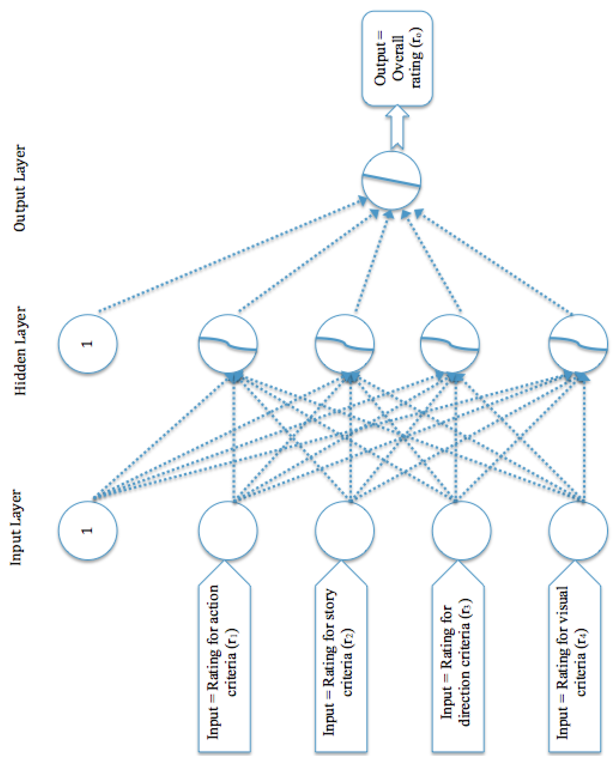
Figure 2.
Class diagram of the model.

Figure 3.
MSE against different values of the learning rate.

Figure 4.
Curve of actual rating from the data set.
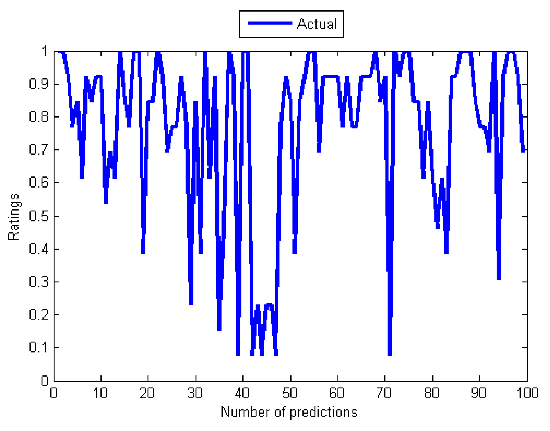
Figure 5.
Graph of actual ratings and the predicted ratings of the experimented algorithms.
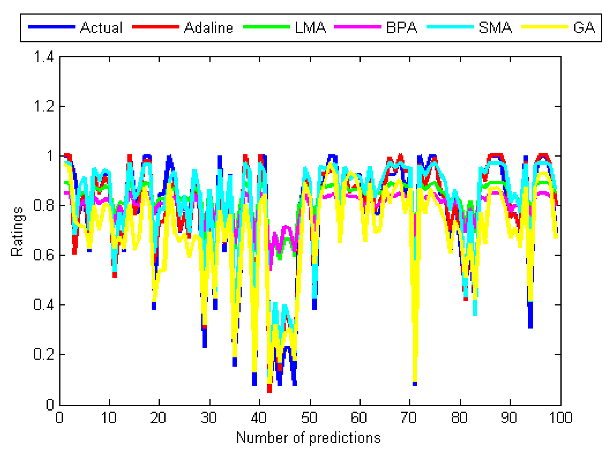
Figure 6.
Curves of actual ratings and predicted ratings of Adaline.

Figure 7.
Curves of actual ratings and predicted ratings of SMA.

Figure 8.
Curves of actual ratings and predicted ratings of LMA.

Figure 9.
Curves of actual ratings and predicted ratings of BPA.
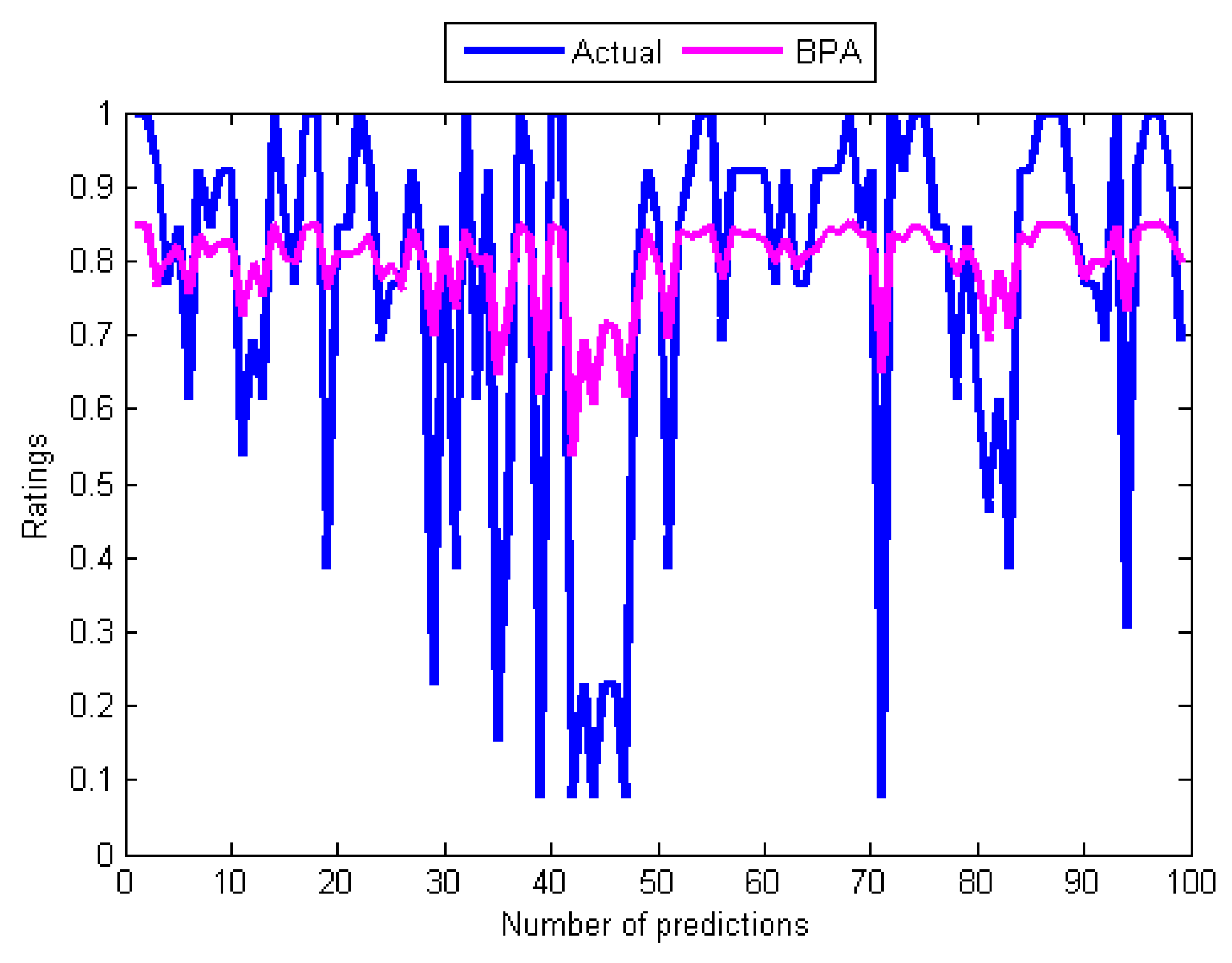
Figure 10.
Curves of actual ratings and predicted ratings of GA.

Figure 11.
Error Performance measure during training with the SMA.


Table 1.
Sample of the Yahoo!Movies data det for multi-criteria recommender systems.
| User ID | Acting | Story | Direction | Visual | Overall | Movie ID |
|---|---|---|---|---|---|---|
| () | () | () | () | () | ||
| 1 | C | C | A | 1 | ||
| B | 0 | B | 2 | |||
| C | 0 | 47 | ||||
| 2 | 0 | 3 | ||||
| A | 0 | B | 4 | |||
| C | 0 | 5 | ||||
| 3 | A | A | 0 | 6 | ||
| B | 4 | |||||
| B | B | 3 |
Table 2.
Modified sample of the Yahoo!Movies data set for multi-criteria recommender systems.
| User ID | Acting | Story | Direction | Visual | Overall | Movie ID |
|---|---|---|---|---|---|---|
| () | () | () | () | () | ||
| 1 | 6 | 6 | 8 | 12 | 8 | 1 |
| 9 | 11 | 10 | 9 | 10 | 2 | |
| 13 | 6 | 5 | 8 | 5 | 47 | |
| 2 | 13 | 13 | 13 | 13 | 13 | 3 |
| 8 | 12 | 11 | 9 | 13 | 4 | |
| 5 | 6 | 13 | 13 | 13 | 5 | |
| 3 | 12 | 10 | 12 | 10 | 10 | 6 |
| 9 | 9 | 10 | 10 | 10 | 4 | |
| 9 | 10 | 9 | 10 | 10 | 3 |
Table 3.
Statistical analysis of the data.
| Measure | Acting | Story | Direction | Visual |
|---|---|---|---|---|
| Correlation | 0.904645 | 0.865350 | 0.910920 | 0.833844 |
| Covariance | 0.065629 | 0.058301 | 0.065686 | 0.055819 |
| p-Value | 0.00000 | 1.44 × 10⁻¹⁵ | 0.00000 | 3.73 × 10⁻²⁹ |
Table 4.
Statistical Analysis of the Experimental result.
| Algorithms | Number of | Average | Average | p-Value |
|---|---|---|---|---|
| Training Cycles | Training MSE | Test MSE | ||
| Adaline | 10 | 0.0054 | 0.0053 | 8.7 × 10−59 |
| SMA | 460 | 0.0075 | 0.0069 | 2.3 × 10−57 |
| GA | 70 | 0.0145 | 0.0138 | 1.4 × 10−55 |
| LMA | 750 | 0.0514 | 0.0389 | 5.4 × 10−52 |
| BPA | 2197 | 0.0509 | 0.0437 | 8.6 × 10−49 |
Table 5.
Correlations between Experimental results.
| Actual | Adeline | LMA | BPA | SMA | GA | |
|---|---|---|---|---|---|---|
| Actual | 1.00 | 0.97 | 0.82 | 0.80 | 0.96 | 0.94 |
| Adaline | 0.97 | 1.00 | 0.86 | 0.85 | 0.99 | 0.96 |
| LMA | 0.82 | 0.86 | 1.00 | 0.97 | 0.88 | 0.90 |
| BPA | 0.80 | 0.85 | 0.97 | 1.00 | 0.86 | 0.87 |
| SMA | 0.96 | 0.99 | 0.88 | 0.86 | 1.00 | 0.97 |
| GA | 0.94 | 0.96 | 0.90 | 0.87 | 0.97 | 1.00 |
© 2017 by the authors. Licensee MDPI, Basel, Switzerland. This article is an open access article distributed under the terms and conditions of the Creative Commons Attribution (CC BY) license (http://creativecommons.org/licenses/by/4.0/).
Share and Cite
MDPI and ACS Style
Hassan, M.; Hamada, M. Performance Comparison of Feed-Forward Neural Networks Trained with Different Learning Algorithms for Recommender Systems. Computation 2017, 5, 40. https://doi.org/10.3390/computation5030040
AMA Style
Hassan M, Hamada M. Performance Comparison of Feed-Forward Neural Networks Trained with Different Learning Algorithms for Recommender Systems. Computation. 2017; 5(3):40. https://doi.org/10.3390/computation5030040
Chicago/Turabian StyleHassan, Mohammed, and Mohamed Hamada. 2017. "Performance Comparison of Feed-Forward Neural Networks Trained with Different Learning Algorithms for Recommender Systems" Computation 5, no. 3: 40. https://doi.org/10.3390/computation5030040
Note that from the first issue of 2016, this journal uses article numbers instead of page numbers. See further details here.