A Diagonally Updated Limited-Memory Quasi-Newton Method for the Weighted Density Approximation


Department of Chemistry & Chemical Biology; McMaster University, Hamilton, ON L8S 4L8, Canada
*
Author to whom correspondence should be addressed.
Computation 2017, 5(4), 42; https://doi.org/10.3390/computation5040042
Submission received: 31 August 2017
/
Revised: 22 September 2017
/
Accepted: 23 September 2017
/
Published: 26 September 2017
(This article belongs to the Special Issue In Memory of Walter Kohn—Advances in Density Functional Theory)
Abstract
:We propose a limited-memory quasi-Newton method using the bad Broyden update and apply it to the nonlinear equations that must be solved to determine the effective Fermi momentum in the weighted density approximation for the exchange energy density functional. This algorithm has advantages for nonlinear systems of equations with diagonally dominant Jacobians, because it is easy to generalize the method to allow for periodic updates of the diagonal of the Jacobian. Systematic tests of the method for atoms show that one can determine the effective Fermi momentum at thousands of points in less than fifteen iterations.
1. Introduction
The accuracy and scope of density functional theory calculations is limited by the need to approximate the density functionals for the exchange-correlation energy [1,2,3,4]. This motivates the robust stream of research into exchange-correlation functionals and the development of new strategies for approximating the exchange-correlation energy. Based on the realization that local and semilocal forms for the exchange-correlation energy functional will always give qualitatively incorrect results for some systems [5,6,7,8,9,10,11,12,13], there has been significant recent work on developing nonlocal density functionals. Some of this work reexamines the very first strategy for nonlocal density functional: the weighted density approximation [14,15,16,17]. The goal of this work is to present a new diagonally updated limited-memory quasi-Newton method we developed for solving a system of nonlinear equations associated with the weighted density approximation. In the remainder of this section, we present background material on the weighted density approximation, so that the nature of the system of nonlinear equations we are solving is clear. (In particular, the system of nonlinear equations is very large, but the Jacobian is dominated by contributions from its diagonal.) Section 2 presents the new method we developed.
For simplicity, in this paper we will consider only the weighted density approximation for the exchange energy, although weighted density approximations for the exchange-correlation and kinetic energy are also available [11,18,19,20,21,22,23,24,25,26,27,28,29,30,31,32,33,34,35,36]. The basic strategy of the weighted density approximation for the exchange energy is to approximate the exchange hole for the electrons,
where is the one-electron reduced density matrix of the noninteracting Kohn-Sham reference system with electron spin-density . The exchange energy of σ-spin electrons can be computed from electron spin-density and the exchange hole,
Many of the failures of modern density functionals are associated with the self-interaction errors that afflict traditional approaches to designing approximate functionals [37,38,39,40]. One advantage of the weighted density approximation is that the self-interaction error is eliminated by explicitly imposing the normalization of the exchange hole,
When Equation (3) holds, the exchange(-correlation) potential has the correct asymptotic decay [38,41,42,43,44,45]. This helps to explain why weighted density approximations tend to give more accurate excitation energies, band gaps, and frontier molecular orbital energies than traditional semilocal density functional approximations [36,46,47,48,49,50,51,52,53,54,55,56,57]. The relatively simple version of the weighted density approximation we consider here is not especially accurate (because the exchange hole is more localized than it should be), but its biggest disadvantage is its high computational cost. A similar normalization requirement to Equation (3), when applied to the direct correlation function, allows one to build nonlocal exchange-correlation holes, which is a promising strategy for increasing the accuracy of the weighted density approximation [19,20,58]. In this contribution, we shall focus instead on reducing the computational cost of weighted density approximation calculations.
Inspired by the mathematical treatment of the nearly uniform electron gas, it is traditional (albeit not ubiquitous [19,20,36,58,59,60,61,62]) to approximate the exchange hole as a function of the form
where is interpreted as the effective Fermi momentum associated with an electron configuration with -spin electrons at positions and . We shall choose to have the form appropriate for the uniform electron gas, namely
This ensures that the uniform-electron gas limit is retained. Garcia-Gonzalez et al. proposed modelling the two-point effective Fermi momentum, , as the power-mean of the effective Fermi momentum at the points separately [27,63],
In this study, we use p = 0.001, which is very close to the geometric mean. (We confirmed that our qualitative conclusions are valid for all 0 < p ≤ .) The multidimensional integrals in Equations (2) and (3) were evaluated numerically, using Becke–Lebedev quadrature [64].
The impediment to the widespread adoption of the weighted density approximation is its computational cost. The normalization constraint for the exchange hole, Equation (3), must be imposed at every point on the numerical integration grid, and evaluating the normalization integral at each point requires a three-dimensional numerical integration. For typical atoms and molecules, determining the effective Fermi momentum requires solving a nonlinear system of ~104–106 equations (Equation (3) at each grid point) with respect to the same number of unknowns ( at each grid point), subject to an inequality constraint at each grid point ( > 0, because it is physically absurd for the Fermi momentum to be nonpositive). Moreover, each of the nonlinear equations is relatively expensive to evaluate, since it requires a numerical integration.
The traditional approach to density-functional theory avoids this problem by performing the integral over r′ in Equation (2) analytically, defining the exchange-correlation energy density,
An alternative, but more convenient, intermediate quantity is the system-averaged spherically-averaged exchange charge,
where denotes integration over the solid angle associated with . ( is often called the system-averaged spherically-averaged exchange hole, but we prefer to distinguish between the exchange hole, , and the exchange charge, , which is the charge that is depleted due to the presence of an electron at .) The exchange-correlation energy can then be evaluated using
The normalization constraint is applied at the level of the functional by requiring that the system-averaged spherically-averaged exchange charge is normalized,
Equation (10) is a far weaker constraint than Equation (3), as it only requires normalization in an average sense. When the electron density is (nearly) uniform, its behavior at one point in space is representative of its system average, imposing Equation (10) (nearly) removes the self-interaction error. This is not true for systems like atoms and molecules, where the chemically relevant regions of the electron density vary over many orders of magnitude. This is clear from the observation that the weighted density approximation using Equation (5) gives results that are quite different from the uniform density approximation, which is obtained if one assumes a homogeneous electron density and performs the integral in Equation (7) analytically to obtain an approximate formula for the exchange energy [18,65].
Motivated by our desire to explore the weighted density approximation in more detail, in the next section, we will present a diagonally-updated limited memory bad Broyden method that allows us to solve the large system of nonlinear equations associated with the weighted density approximation in a computationally efficient manner. Then we present the results of a numerical test of this method (Section 3) and discuss its implications and the possibilities for further improvement (Section 4).
2. Methods
The methods we shall use for solving the nonlinear equations for the weighted density approximation are generally applicable, so we will first rewrite the problem (cf. Equations (3)–(6)) in a general form. Suppose there are G points in the numerical integration grid, . The unknown is the value of the Fermi momentum at each of these points, which we denote . Because the equations for the different spins are decoupled, we shall simplify our notation by omitting the spin-index, σ. There is a nonlinear equation for each grid point also, which has the form,
where
Here denote the numerical integration weights. The Jacobian for this system of equations is defined as
Using Newton’s method, one could then define an update for the variables,
where are the elements of the inverse Jacobian matrix, . In matrix-vector notation, Equation (14) can be written as
The method is then repeated using the updated variables to evaluate the equations, (11), and the Jacobian thereof, until convergence is achieved.
In practice, this technique does not always converge. Convergence can be enhanced by scaling the step, using either a trust radius or a line search. Specifically, the update is rewritten as
where ζ is chosen so that the step-size is decreased whenever the Newton update (Equation (15), which is derived by truncating the Taylor series for f(k) at first order) is unreliable.
For large systems of or more equations, evaluating and inverting the Jacobian for each Newton iteration, Equation (16), is prohibitively expensive. This motivates quasi-Newton methods, where the Jacobian or its inverse is approximated. One of the simplest quasi-Newton methods is to evaluate only the diagonal elements of the Jacobian,
The inverse of a diagonal matrix is simply the inverse of its diagonal elements, so this gives a very simple update formula,
The system of equations associated with the weighted density approximation, Equation (12), gives a Jacobian that is strongly diagonally dominant, so this formula is appropriate for our application, and we shall test it in Section 3.
One can often improve the simple diagonal update formula if one uses information from previous iterations. As an example, suppose one has the function and argument values from several previous iterations, and , respectively. (Here and in the following, we use to denote the equations evaluated at the argument , .) If the vector is short enough, then
These secant conditions can be used to improve an initial estimate for the Jacobian (Equation (19)) or inverse Jacobian (Equation (20)). The best-known methods for doing this are the methods proposed by Broyden [66,67],
where
and, more generally, we define
The Jacobian in Equation (21) is usually called the Broyden update for the Jacobian. The method based on the inverse Jacobian, Equation (22), is usually called the “bad” Broyden method because in its original applications, it did not perform as well as the “good” Broyden update, Equation (21) [66,68,69,70,71,72]. It is more convenient to have an update to the inverse Jacobian than the Jacobian itself since (cf. Equation (16)) otherwise one needs to solve a (large) system of linear equations to determine the step. Fortunately, the “good” Broyden update can also be formulated as an update to the inverse Jacobian,
Storing the entire (inverse) quasi-Newton Jacobian matrix is impractical for large systems of nonlinear equations, but fortunately one only needs to know the action of the inverse-Jacobian matrix on the vector to compute the updated step. Furthermore, we can decide to store only the results of the last few updates, Equations (23) and (24). With such a procedure, one can control the computational cost and amount of memory required to compute the quasi-Newton update.
The remainder of this section presents the limited-memory “bad” Broyden method we developed for the weighted density approximation. Specifically, we noticed that the “bad” Broyden method has an especially simple quasi-Newton update. Suppose one has an initial guess for the inverse Jacobian, . The action of the inverse quasi-Newton Jacobian on can then be computed recursively. One starts with the initialization,
and then refines the Jacobian according to the recursion,
One can include as many previous steps from Equations (23) and (24) as one wishes, but because it is most effective to update the inverse Jacobian using local information; including too much previous information not only increases the computational cost, but often degrades the accuracy of the approximation. If the data from s previous steps are included, then the action of the quasi-Newton inverse Hessian is computed by
This is the limited-memory bad Broyden procedure we developed to solve Equations (11) and (12).
To make this procedure practical, we introduce two additional refinements. First, we can periodically update the approximate inverse-Jacobian that is used in Equation (30) using, for example, the diagonal approximation to the Jacobian (which is relatively easy to compute for the weighted density approximation). Second, we introduce a global trust radius to control the stepsize. We also tried using a local trust radius, where each component of the step could be scaled separately, but this did not improve our results. Suppose the trust radius for step m is . Then we will take the full quasi-Newton step if the norm of the step is shorter than the trust radius, . Otherwise, we (1) scale back the step so that it is the same size as the trust radius,
and (2) because it is physically absurd to have a negative effective Fermi momentum; we never let the Fermi momentum at any grid point decrease by a factor of more than two in any iteration,
Here denote the elements of the updated Fermi momentum from Equation (31). Next we then check to see if the total absolute error in the nonlinear system decreased; otherwise we reject the step and try again with a step size equal to half the previous stepsize. That is, we evaluate and if , then we reject the step and try again with
If the step is accepted, then we need to update the trust radius. The basic idea is that if the sign of the objective function changes, , then we overshot the solution of the gth nonlinear equation. We therefore let each grid point “vote” on whether it thought the last step was too long (), too short (), or about right. Let denote the number of too-long steps, denote the number of too-short steps, and denote the length of the previous step. We then update the trust radius based on whether the consensus seems to be that the trust radius was too short or too long. Specifically,
The three cases in this formula correspond to cases where the step was too short for most grid points, too long for most grid points, or “about right”. Equation (34) can be thought of as a trust-radius update based on the norm.
3. Results
We tested the limited-memory bad Broyden method from Section 2 by solving the weighted density approximation for the neutral atoms, H–Kr, with p = 0.001 (cf. Equation (12)). We tested the method storing up to 10 previous steps (s = 1, 2, …, 10 in Equation (30)), using the diagonal approximation to the Jacobian (cf. Equation (17)) to estimate (cf. Equation (30)). We also considered updating the diagonal inverse-Jacobian approximation every t iterations (t = 1, 2, …, 5). For our tests, it was fastest to use 8 previous steps (s = 8) and to update the approximate inverse Jacobian every other iteration (t = 2). The nonlinear equations were considered converged when the error in every equation was less than 10−3.
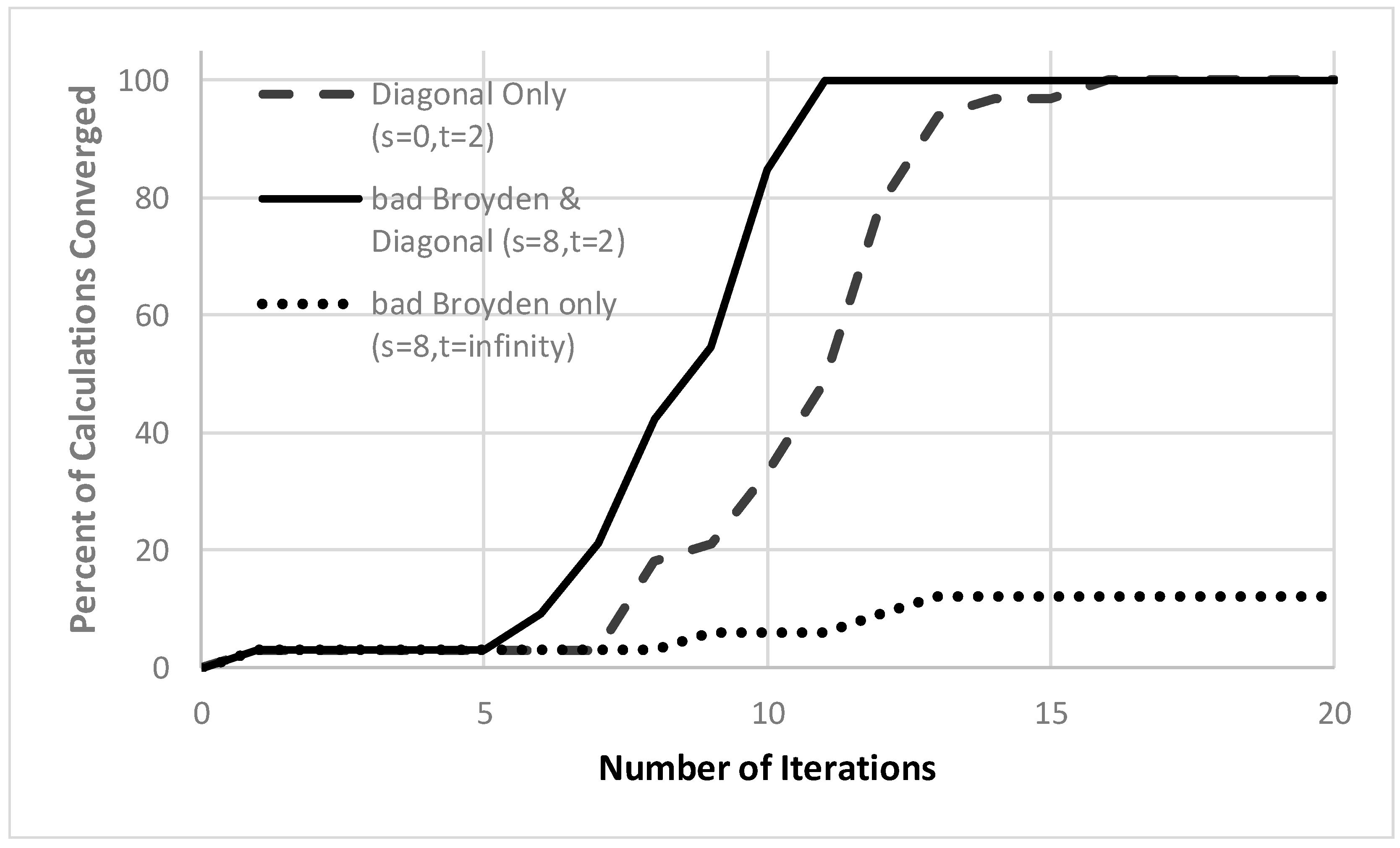
In Figure 1, we report key results. The bad Broyden method by itself is quite poor, converging less than 15% of the calculations in 20 iterations, and only 60% of the calculations within 200 iterations. By contrast, because the Jacobian is diagonally dominant, using the diagonal Jacobian (and updating it in every other iteration) converges all the atoms within 16 iterations. The best method of all starts with the diagonal update, but then improves the model using the limited memory bad Broyden update retaining 8 vectors. With that method, all the atoms are converged in just 11 iterations. We also tested the method for different hole correlation models (the Gaussian model [65] and the exchange-correlation hole of the uniform electron gas [11,73]) and for various values of p. The results are very similar, with the bad Broyden method with periodic diagonal updates performing the best. As the p value in Equation (12) increases, the equations become increasingly difficult to converge, though up until convergence is achieved in less than ~20 iterations. When , the algorithm seems to do an acceptable job of finding a least-squares solution that almost satisfies the nonlinear equations, which do not seem to have any solution [11,18].
The computational cost of the method is dominated by the evaluation of the objective function (Equation (12)) at each grid point and the computation of the diagonal elements of the Jacobian, which has almost exactly the same cost as evaluating the objective function. This is why we compute the diagonal elements of the Jacobian only in every other iteration instead of every iteration; the incremental increase in convergence rate obtained by computing the Jacobian’s diagonal each iteration is not worth the additional computational expense. The actual computation of the bad Broyden update, Equations (28)–(30), is comparatively insignificant, partly because it can be efficiently evaluated using the (precomputed) quantities ().
Based on these results, it seems the diagonally-updated limited-memory bad Broyden method is ideally suited for the problem of solving the weighted density approximation equations, (12), and is presumably useful for other similarly large, diagonally dominant systems of nonlinear equations as well.
4. Discussion
Despite its theoretical promise, applications of the weighted density approximation have been limited by the difficulty of solving the nonlinear equations for the local effective Fermi momentum in the weighted density approximation (cf. Equation (12)). Because there is one nonlinear equation for each grid point, and evaluating each equation requires an integration over all space, this is an extremely challenging numerical problem. It is not uncommon to have ~104–106 grid points, and having fewer than ~103 grid points is extremely rare. We developed a limited-memory quasi-Newton method, which we believe will be useful also in other contexts, based on a recursive formulation of the bad Broyden update, built upon an approximate inverse-Jacobian (which we update every other iteration using the diagonal approximation for the Jacobian). For the atoms H–Kr, this method always converged in 11 or fewer iterations.
There are two ways to improve this model. First, we can reduce the number of nonlinear equations to be solved. It is reasonable to expect, for example, that after solving Equations (11) for enough grid points, accurate results for the effective Fermi momentum at the other grid points could be obtained by interpolation. Second, we could improve the quasi-Newton method itself. One possibility would be to notice that the same recursive method we developed for the bad Broyden method could be used for the good Broyden method, (21), simply by interchanging the roles of and . That method, however, still requires solving the equations for the step-size. Another possibility is that instead of sequentially updating the Jacobian, we could use a multisecant update [74]. In particular, defining the matrices whose columns are determined from the previous steps,
we can write a multisecant update for the bad Broyden method as:
and for the good Broyden method as
The matrix inversions in Equations (37) and (38) should be viewed as generalized (Moore–Penrose) inverses. We believe that Equation (38) is the most reasonable way to implement a limited-memory good Broyden method, but we have not implemented or tested this method because we doubt it is possible to greatly improve upon the results we obtained for the limited-memory bad Broyden method with periodic diagonal updates (as shown in Figure 1).
Acknowledgments
Research support from Compute Canada, NSERC, and the Canada Research Chairs is gratefully acknowledged.
Author Contributions
M.C. performed the calculations. M.C., P.A., R.C.-S. and D.C. analyzed the data. P.A. designed the algorithm and implemented the method into a program that was later modified by D.C. and R.C.-S. M.C. and P.A. designed the computational study. P.A. wrote the paper, with assistance from M.C. and D.C.
Conflicts of Interest
The authors declare no conflicts of interest.
References
- Cohen, A.J.; Mori-Sanchez, P.; Yang, W.T. Challenges for density functional theory. Chem. Rev. 2012, 112, 289–320. [Google Scholar] [CrossRef] [PubMed]
- Perdew, J.P.; Ruzsinszky, A.; Tao, J.M.; Staroverov, V.N.; Scuseria, G.E.; Csonka, G.I. Prescription for the design and selection of density functional approximations: More constraint satisfaction with fewer fits. J. Chem. Phys. 2005, 123, 062201. [Google Scholar] [CrossRef] [PubMed]
- Cohen, A.J.; Mori-Sanchez, P.; Yang, W.T. Insights into current limitations of density functional theory. Science 2008, 321, 792–794. [Google Scholar] [CrossRef] [PubMed]
- Parr, R.G.; Yang, W. Density-Functional Theory of Atoms and Molecules; Oxford UP: New York, NY, USA, 1989. [Google Scholar]
- Savin, A. On degeneracy, near-degeneracy, and density functional theory. In Recent Developments and Applications of Modern Density Functional Theory; Seminario, J.M., Ed.; Elsevier: New York, NY, USA, 1996; p. 327. [Google Scholar]
- Gori-Giorgi, P.; Savin, A. Degeneracy and size consistency in electronic density functional theory. In Ab Initio Simulation of Crystalline Solids: History and Prospects—Contributions in Honor of Cesare Pisani; Dovesi, R., Orlando, R., Roetti, C., Eds.; IOP: Bristol, UK, 2008; Volume 117, p. 12017. [Google Scholar]
- Savin, A. Is size-consistency possible with density functional approximations? Chem. Phys. 2009, 356, 91–97. [Google Scholar] [CrossRef]
- Ayers, P.W.; Levy, M. Tight constraints on the exchange-correlation potentials of degenerate states. J. Chem. Phys. 2014, 140, 18a537. [Google Scholar] [CrossRef] [PubMed]
- Levy, M.; Anderson, J.S.M.; Heidar-Zadeh, F.H.; Ayers, P.W. Kinetic and electron-electron energies for convex sums of ground state densities with degeneracies and fractional electron number. J. Chem. Phys. 2014, 140, 18a538. [Google Scholar] [CrossRef] [PubMed]
- Merkle, R.; Savin, A.; Preuss, H. Singly ionized 1st-row dimers and hydrides calculated with the fully numerical density-functional program numol. J. Chem. Phys. 1992, 97, 9216–9221. [Google Scholar] [CrossRef]
- Cuevas-Saavedra, R.; Chakraborty, D.; Rabi, S.; Cardenas, C.; Ayers, P.W. Symmetric non local weighted density approximations from the exchange-correlation hole of the uniform electron gas. J. Chem. Theory Comp. 2012, 8, 4081–4093. [Google Scholar] [CrossRef] [PubMed]
- Perdew, J.P. What do the kohn-sham orbital energies mean? How do atoms dissociate? NATO ASI Ser. 1985, 123, 265–308. [Google Scholar]
- Mori-Sanchez, P.; Cohen, A.J.; Yang, W.T. Discontinuous nature of the exchange-correlation functional in strongly correlated systems. Phys. Rev. Lett. 2009, 102, 066403. [Google Scholar] [CrossRef] [PubMed]
- Chacon, E.; Tarazona, P. Self-consistent weighted-density approximation for the electron-gas 1. Bulk properties. Phys. Rev. B 1988, 37, 4013–4019. [Google Scholar] [CrossRef]
- Alonso, J.A.; Girifalco, L.A. Nonlocal approximation to exchange energy of non-homogenous electron-gas. Solid State Commun. 1977, 24, 135–138. [Google Scholar] [CrossRef]
- Alonso, J.A.; Girifalco, L.A. Nonlocal approximation to exchange potential and kinetic-energy of an inhomogeneous electron-gas. Phys. Rev. B 1978, 17, 3735–3743. [Google Scholar] [CrossRef]
- Gunnarsson, O.; Jonson, M.; Lundqvist, B.I. Exchange and correlation in inhomogeneous electron-systems. Solid State Commun. 1977, 24, 765–768. [Google Scholar] [CrossRef]
- Cuevas-Saavedra, R.; Chakraborty, D.; Ayers, P.W. Symmetric two-point weighted density approximation for exchange energies. Phys. Rev. A 2012, 85. [Google Scholar] [CrossRef]
- Cuevas-Saavedra, R.; Thompson, D.C.; Ayers, P.W. Alternative ornstein-zernike models from the homogeneous electron liquid for density functional theory calculations. Int. J. Quantum Chem. 2016, 116, 852–861. [Google Scholar] [CrossRef]
- Cuevas-Saavedra, R.; Ayers, P.W. Using the spin-resolved electronic direct correlation function to estimate the correlation energy of the spin-polarized uniform electron gas. J. Phys. Chem. Solids 2012, 73, 670–673. [Google Scholar] [CrossRef]
- Ayers, P.W.; Cuevas-Saavedra, R.; Chakraborty, D. A variational principle for the electron density using the exchange hole & its implications for n-representability. Phys. Lett. A 2012, 376, 839–844. [Google Scholar]
- Cuevas-Saavedra, R.; Ayers, P.W. Addressing the coulomb potential singularity in exchange-correlation energy integrals with one-electron and two-electron basis sets. Chem. Phys. Lett. 2012, 539, 163–167. [Google Scholar] [CrossRef]
- Antaya, H.; Zhou, Y.X.; Ernzerhof, M. Approximating the exchange energy through the nonempirical exchange-factor approach. Phys. Rev. A 2014, 90, 032513. [Google Scholar] [CrossRef]
- Patrick, C.E.; Thygesen, K.S. Adiabatic-connection fluctuation-dissipation dft for the structural properties of solids-the renormalized alda and electron gas kernels. J. Chem. Phys. 2015, 143, 102802. [Google Scholar] [CrossRef] [PubMed]
- Zhou, Y.X.; Bahmann, H.; Ernzerhof, M. Construction of exchange-correlation functionals through interpolation between the non-interacting and the strong-correlation limit. J. Chem. Phys. 2015, 143, 124103. [Google Scholar] [CrossRef] [PubMed]
- Precechtelova, J.P.; Bahmann, H.; Kaupp, M.; Ernzerhof, M. Design of exchange-correlation functionals through the correlation factor approach. J. Chem. Phys. 2015, 143, 144102. [Google Scholar]
- GarciaGonzalez, P.; Alvarellos, J.E.; Chacon, E. Kinetic-energy density functional: Atoms and shell structure. Phys. Rev. A 1996, 54, 1897–1905. [Google Scholar] [CrossRef]
- Garcia-Aldea, D.; Alvarellos, J.E. Kinetic-energy density functionals with nonlocal terms with the structure of the thomas-fermi functional. Phys. Rev. A 2007, 76, 052504. [Google Scholar] [CrossRef]
- Garcia-Aldea, D.; Alvarellos, J.E. Approach to kinetic energy density functionals: Nonlocal terms with the structure of the von weizsacker functional. Phys. Rev. A 2008, 77, 022502. [Google Scholar] [CrossRef]
- Garcia-Aldea, D.; Alvarellos, J.E. Fully nonlocal kinetic energy density functionals: A proposal and general assessment for atomic systems. J. Chem. Phys. 2008, 129, 074103. [Google Scholar] [CrossRef] [PubMed]
- Garcia-Gonzalez, P.; Alvarellos, J.E.; Chacon, E. Kinetic-energy density functionals based on the homogeneous response function applied to one-dimensional fermion systems. Phys. Rev. A 1998, 57, 4192–4200. [Google Scholar] [CrossRef]
- Wang, Y.A.; Govind, N.; Carter, E.A. Orbital-free kinetic-energy density functionals with a density-dependent kernel. Phys. Rev. B 1999, 60, 16350–16358. [Google Scholar] [CrossRef]
- Wang, Y.A.; Carter, E.A.; Schwartz, S.D. Orbital-free kinetic-energy density functional theory. In Theoretical Methods in Condensed Phase Chemistry; Kluwer: Dordrecht, The Netherlands, 2000; pp. 117–184. [Google Scholar]
- Zhou, B.J.; Ligneres, V.L.; Carter, E.A. Improving the orbital-free density functional theory description of covalent materials. J. Chem. Phys. 2005, 122, 044103. [Google Scholar] [CrossRef] [PubMed]
- Garcia-Gonzalez, P.; Alvarellos, J.E.; Chacon, E. Nonlocal symmetrized kinetic-energy density functional: Application to simple surfaces. Phys. Rev. B 1998, 57, 4857–4862. [Google Scholar] [CrossRef]
- Rushton, P.P.; Tozer, D.J.; Clark, S.J. Nonlocal density-functional description of exchange and correlation in silicon. Phys. Rev. B 2002, 65, 235203. [Google Scholar] [CrossRef]
- Gori-Giorgi, P.; Angyan, J.G.; Savin, A. Charge density reconstitution from approximate exchange-correlation holes. Can. J. Chem. 2009, 87, 1444–1450. [Google Scholar] [CrossRef]
- Perdew, J.P.; Zunger, A. Self-interaction correction to density-functional approximations for many-electron systems. Phys. Rev. B 1981, 23, 5048–5079. [Google Scholar] [CrossRef]
- Gunnarsson, O.; Jones, R.O. Self-interaction corrections in the density functional formalism. Solid State Commun. 1981, 37, 249–252. [Google Scholar] [CrossRef]
- Perdew, J.P. Orbital functional for exchange and correlation—Self-interaction correction to the local density approximation. Chem. Phys. Lett. 1979, 64, 127–130. [Google Scholar] [CrossRef]
- Almbladh, C.O.; Von Barth, U. Exact results for the charge and spin-densities, exchange- correlation potentials, and density-functional eigenvalues. Phys. Rev. B 1985, 31, 3231–3244. [Google Scholar] [CrossRef]
- Levy, M.; Perdew, J.P.; Sahni, V. Exact differential-equation for the density and ionization- energy of a many-particle system. Phys. Rev. A 1984, 30, 2745–2748. [Google Scholar] [CrossRef]
- Qian, Z.X.; Sahni, V. Analytical asymptotic structure of the pauli, coulomb, and correlation-kinetic components of the kohn-sham theory exchange-correlation potential in atoms. Int. J. Quantum Chem. 1998, 70, 671–680. [Google Scholar] [CrossRef]
- Qian, Z.X.; Sahni, V. Analytical properties of the kohn-sham theory exchange and correlation energy and potential via quantal density functional theory. Int. J. Quantum Chem. 2000, 80, 555–566. [Google Scholar] [CrossRef]
- Ayers, P.W.; Levy, M. Sum rules for exchange and correlation potentials. J. Chem. Phys. 2001, 115, 4438–4443. [Google Scholar] [CrossRef]
- Tozer, D.J.; Handy, N.C. Improving virtual kohn-sham orbitals and eigenvalues: Application to excitation energies and static polarizabilities. J. Chem. Phys. 1998, 109, 10180–10189. [Google Scholar] [CrossRef]
- Tozer, D.J. Relationship between long-range charge-transfer excitation energy error and integer discontinuity in kohn-sham theory. J. Chem. Phys. 2003, 119, 12697–12699. [Google Scholar] [CrossRef]
- Wu, Q.; Ayers, P.W.; Yang, W.T. Density-functional theory calculations with correct long-range potentials. J. Chem. Phys. 2003, 119, 2978–2990. [Google Scholar] [CrossRef]
- Dreuw, A.; Weisman, J.L.; Head-Gordon, M. Long-range charge-transfer excited states in time-dependent density functional theory require non-local exchange. J. Chem. Phys. 2003, 119, 2943–2946. [Google Scholar] [CrossRef]
- Andrade, X.; Aspuru-Guzik, A. Prediction of the derivative discontinuity in density functional theory from an electrostatic description of the exchange and correlation potential. Phys. Rev. Lett. 2011, 107, 183002. [Google Scholar] [CrossRef] [PubMed]
- Ayers, P.W.; Morrison, R.C.; Parr, R.G. Fermi-amaldi model for exchange-correlation: Atomic excitation energies from orbital energy differences. Mol. Phys. 2005, 103, 2061–2072. [Google Scholar] [CrossRef]
- Savin, A.; Umrigar, C.J.; Gonze, X. Relationship of kohn-sham eigenvalues to excitation energies. Chem. Phys. Lett. 1998, 288, 391–395. [Google Scholar] [CrossRef]
- Balbas, L.C.; Alonso, J.A.; Rubio, A. One-electron energy eigenvalues in the weighted-density approximation to exchange and correlation. Europhys. Lett. 1991, 14, 323–329. [Google Scholar] [CrossRef]
- Robertson, J.; Xiong, K.; Clark, S.J. Band structure of functional oxides by screened exchange and the weighted density approximation. Phys. Status Solidi B 2006, 243, 2054–2070. [Google Scholar] [CrossRef]
- Wu, Z.G.; Singh, D.J.; Cohen, R.E. Electronic structure of calcium hexaboride within the weighted density approximation. Phys. Rev. B 2004, 69, 193105. [Google Scholar] [CrossRef]
- Wu, Z.G.; Cohen, R.E.; Singh, D.J.; Gupta, R.; Gupta, M. Weighted-density-approximation description of rare-earth trihydrides. Phys. Rev. B 2004, 69, 085104. [Google Scholar] [CrossRef]
- Zheng, G.; Clark, S.J.; Brand, S.; Abram, R.A. Non-local density functional description of poly-para-phenylene vinylene. Chin. Phys. Lett. 2007, 24, 807–810. [Google Scholar]
- Cuevas-Saavedra, R.; Ayers, P.W. Exchange-correlation functionals from the identical-particle ornstein-zernike equation: Basic formulation and numerical algorithms. In Condensed Matter Theory; Ludena, E.V., Bishop, R.F., Iza, P., Eds.; World Scientific: Singapore, 2011; Volume 25. [Google Scholar]
- Becker, M.S. Integrodifferential equation for the ground state of an electron gas. Phys. Rev. 1969, 185, 168–171. [Google Scholar] [CrossRef]
- March, N.H. Boson and fermion many-body assemblies: Fingerprints of excitations in the ground-state wave functions, with examples of superfluid He-4 and the homogeneous correlated electron liquid. Phys. Chem. Liq. 2008, 46, 465–480. [Google Scholar] [CrossRef]
- Amovilli, C.; March, N.H. Ornstein-zernike function and coulombic correlation in the homogeneous electron liquid. Phys. Rev. B 2007, 76, 195104. [Google Scholar] [CrossRef]
- Cuevas-Saavedra, R.; Ayers, P.W. Exchange-correlation functionals from the identical-particle ornstein-zernike equation: Basic formulation and numerical algorithms. Int. J. Mod. Phys. B 2010, 24, 5115–5127. [Google Scholar] [CrossRef]
- Garcia-Gonzalez, P.; Alvarellos, J.E.; Chacon, E.; Tarazona, P. Image potential and the exchange-correlation weighted density approximation functional. Phys. Rev. B 2000, 62, 16063–16068. [Google Scholar] [CrossRef]
- Becke, A.D. A multicenter numerical-integration scheme for polyatomic molecules. J. Chem. Phys. 1988, 88, 2547–2553. [Google Scholar] [CrossRef]
- Lee, C.; Parr, R.G. Gaussian and other approximations to the first-order density matrix of electronic systems, and the derivation of various local-density-functional theories. Phys. Rev. A 1987, 35, 2377–2383. [Google Scholar] [CrossRef]
- Broyden, C.G. On the discovery of the "good broyden" method. Math. Program. 2000, 87, 209–213. [Google Scholar] [CrossRef]
- Broyden, C.G. A class of methods for solving nonlinear simultaneous equations. Math. Comput. 1965, 19, 577–593. [Google Scholar] [CrossRef]
- Anglada, J.M.; Bofill, J.M. How good is a broyden-fletcher-goldfarb-shanno-like update hessian formula to locate transition structures? Specific reformulation of broyden-fletcher-goldfarb-shanno for optimizing saddle points. J. Comput. Chem. 1998, 19, 349–362. [Google Scholar] [CrossRef]
- Kvaalen, E. A faster broyden method. BIT 1991, 31, 369–372. [Google Scholar] [CrossRef]
- Griewank, A. Broyden updating, the good and the bad! Doc. Math. 2012, ISMP, 301–315. [Google Scholar]
- Brune, P.R.; Knepley, M.G.; Smith, B.F.; Tu, X. Composing scalable nonlinear algebraic solvers. Siam Rev. 2015, 57, 535–565. [Google Scholar] [CrossRef]
- Al-Baali, M.; Spedicato, E.; Maggioni, F. Broyden‘s quasi-newton methods for a nonlinear system of equations and unconstrained optimization: A review and open problems. Optim. Methods Softw. 2014, 29, 937–954. [Google Scholar] [CrossRef]
- Gori-Giorgi, P.; Perdew, J.P. Pair distribution function of the spin-polarized electron gas: A first-principles analytic model for all uniform densities. Phys. Rev. B 2002, 66, 165118. [Google Scholar] [CrossRef]
- Burger, S.K.; Ayers, P.W. Quasi-newton parallel geometry optimization methods. J. Chem. Phys. 2010, 133, 034116. [Google Scholar] [CrossRef] [PubMed]
Figure 1.
Convergence of quasi-Newton approaches for the weighted density approximation of atoms. The percent of the atoms H–Kr, for which the nonlinear equations in Equation (11) have converged to with 10−3 (vertical axis) within a given number of iterations (horizonal axis). Eight vectors are retained in the bad Broyden update and the diagonal Jacobian is updated every other iteration. The curves show the results for the simplest limited-memory bad Broyden update (with no diagonal update except in the first iteration; dotted line), the limited-memory bad Broyden update (with diagonal updates every other iteration; solid line), and the diagonal approximation to the (inverse) Jacobian updated every other iteration (with no bad Broyden updates; dashed line).
© 2017 by the authors. Licensee MDPI, Basel, Switzerland. This article is an open access article distributed under the terms and conditions of the Creative Commons Attribution (CC BY) license (http://creativecommons.org/licenses/by/4.0/).
Share and Cite
MDPI and ACS Style
Chan, M.; Cuevas-Saavedra, R.; Chakraborty, D.; Ayers, P.W. A Diagonally Updated Limited-Memory Quasi-Newton Method for the Weighted Density Approximation. Computation 2017, 5, 42. https://doi.org/10.3390/computation5040042
AMA Style
Chan M, Cuevas-Saavedra R, Chakraborty D, Ayers PW. A Diagonally Updated Limited-Memory Quasi-Newton Method for the Weighted Density Approximation. Computation. 2017; 5(4):42. https://doi.org/10.3390/computation5040042
Chicago/Turabian StyleChan, Matthew, Rogelio Cuevas-Saavedra, Debajit Chakraborty, and Paul W. Ayers. 2017. "A Diagonally Updated Limited-Memory Quasi-Newton Method for the Weighted Density Approximation" Computation 5, no. 4: 42. https://doi.org/10.3390/computation5040042
Note that from the first issue of 2016, this journal uses article numbers instead of page numbers. See further details here.