Nonlinear-Adaptive Mathematical System Identification


Department of Mechanical Engineering, Stanford University, Stanford, CA 94305, USA
Computation 2017, 5(4), 47; https://doi.org/10.3390/computation5040047
Submission received: 29 September 2017
/
Revised: 23 November 2017
/
Accepted: 28 November 2017
/
Published: 30 November 2017
(This article belongs to the Section Computational Engineering)
Abstract
:By reversing paradigms that normally utilize mathematical models as the basis for nonlinear adaptive controllers, this article describes using the controller to serve as a novel computational approach for mathematical system identification. System identification usually begins with the dynamics, and then seeks to parameterize the mathematical model in an optimization relationship that produces estimates of the parameters that minimize a designated cost function. The proposed methodology uses a DC motor with a minimum-phase mathematical model controlled by a self-tuning regulator without model pole cancelation. The normal system identification process is briefly articulated by parameterizing the system for least squares estimation that includes an allowance for exponential forgetting to deal with time-varying plants. Next, towards the proposed approach, the Diophantine equation is derived for an indirect self-tuner where feedforward and feedback controls are both parameterized in terms of the motor’s math model. As the controller seeks to nullify tracking errors, the assumed plant parameters are adapted and quickly converge on the correct parameters of the motor’s math model. Next, a more challenging non-minimum phase system is investigated, and the earlier implemented technique is modified utilizing a direct self-tuner with an increased pole excess. The nominal method experiences control chattering (an undesirable characteristic that could potentially damage the motor during testing), while the increased pole excess eliminates the control chattering, yet maintains effective mathematical system identification. This novel approach permits algorithms normally used for control to instead be used effectively for mathematical system identification.
1. Introduction
1.1. Background
Nonlinear adaptive controllers, as described in [1], utilize an assumed mathematical structure of the plant to be controlled. Self-tuning regulators that either directly or indirectly parameterize the control in terms of the assumed plan math model are introduced with the goal of improving the tracking performance of the controller. The feedback is parameterized in a Diophantine equation [2], also referred to in the literature as a Bezout identity [3], or, alternatively, as an Aryabhatta equation [4]. Without saying it, this description describes a method of system identification where the identified system parameters are the time-varying terms in a nonlinear adaptive controller. Since the plant’s mathematical model derives from first principles, the plant’s mathematical equation can instead be considered the output of such algorithms, assuming the algorithm demonstrates parameter convergence.
1.2. Literature Review
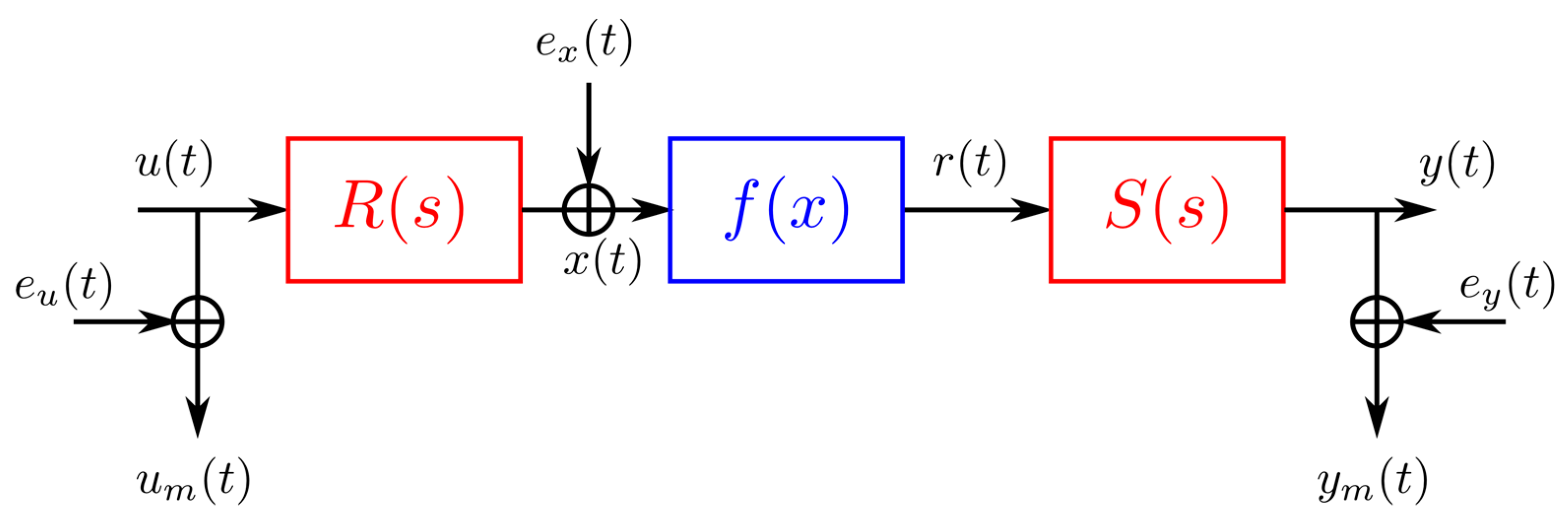
System identification is a mature field that often assumes some knowledge for the plant structure. One such structure is the Wiener–Hammerstein benchmark—a well-known, block-oriented structure containing a static nonlinearity that is sandwiched in between two linear time-invariant (LTI) blocks. This benchmark, depicted in Figure 1, is useful for dominant process noise, but the presence of the two LTI blocks results in a problem that is harder to identify [5,6].
The Bouc–Wen System [8,9] has been intensively exploited during the last decades to represent hysteretic effects in mechanical engineering, especially in the case of random vibrations. A Parallel Wiener–Hammerstein system [10] is obtained by connecting multiple Wiener–Hammerstein systems in parallel. Each parallel branch contains a static nonlinearity that is sandwiched in between two linear time-invariant (LTI) blocks. The presence of the two LTI blocks and the parallel branches results in a problem that is harder to identify. The Silverbox system [11] can be seen as an electronic implementation of the Duffing oscillator (a nonlinear oscillator with a potential energy with both quadratic and cubic terms). It is built as a second-order linear time-invariant system with a third-degree polynomial static nonlinearity around it in feedback. This type of dynamic is, for instance, often encountered in mechanical systems. The standard paradigm involves using the proper method to identify the system being controlled [12,13,14,15,16,17], and parameterizing the controller in terms of the identified variables [18,19,20]. Instead, we consider starting at the controller which is parameterized in terms of the system variables, and investigate the utility of the nonlinear adaptive controller to perform system identification.
1.3. Formulation of the Problem of Interest for This Investigation
Problem formulation is articulated in Section 2, beginning by expressing the mathematical model in linear regression parameterization that permits investigation of exponential forgetting. An indirect self-tuning regulator (including both feedforward and feedback) is then designed without pole excess where a desired closed-loop system response is used to estimate the system parameters. Next, a more challenging non-minimum phase mathematical model is investigated, where the direct self-tuning regulator is used and is permitted pole excess that is presumed to be unknown.
1.4. Contribution of This Study
This study starts at the controller, which is parameterized in terms of the system variables, and investigates the utility of the nonlinear adaptive controller to perform system identification. References [18,19] utilize a continuous implementation of this approach with extended least squares, while this paper articulates a discrete implementation with least squares applied to both minimum phase and non-minimum phase plants.
1.5. Organization of the Paper
With the context of the literature review above in Section 1.2, Section 2 includes a detailed problem formulation described briefly in Section 1.3, and also includes the results that confirm the contribution described in Section 1.4. Finally, Section 3 includes a brief discussion of the results to remind the reader of the qualitative nature of implementation of the methods utilized and results achieved in Section 2.
2. Materials and Methods
The methods in this study stem from methods and problem formulation in [1], whose most recent expressions in the literature in [18,19] implement a continuous form, with excursions to exponential forgetting and posterior residuals in a regression formulation that includes extended least squares, but does not include non-minimum phase plants or discretized system equations. The immediately following sections will establish the discrete parameterized expressions in the same general form as [1,18,19], permitting extension to exponential forgetting, posterior residuals, and extended least squares with implementations on both minimum phase and non-minimum phase plants, where both direct and indirect self-tuning regulator schemes are used as the nominal controller models.
2.1. Minimum Phase System
2.1.1. Parameterization
A DC motor with a plant given in the Laplace domain (indicated by variable s) is represented in Equation (1), which was discretized as Equation (2). This is indicated by the discrete time-shift operator variable q, where t indicates time (shifted in discrete steps (i.e., 1, 2, …, n)) used on the output y side of the equation, and where the pole excess d0 is written in terms of the time-shift operator, requiring a separate index m used on the control u side of the equation. To allow least squares estimation procedures, the discrete process model may be written as Equation (3) (parameterized in Equations (4) and (5)). The parameters are organized into a column-vector θ in Equation (4), and the variables are similarly organized as ϕ in Equation (5), permitting the system to be expressed in a standard regression format whose recursive evaluation is shown in Equation (6), where the estimation error ε (also known as the innovations) is used with time-varying gain terms K(t) written in the form of the error covariance P(t). The estimates of the parameters are denoted by .
The least squares with exponential forgetting algorithm (Equation (6)) is coded per [1], but note that the forgetting factor λ = 1 was used (initially); thus, exponential forgetting was not implemented to permit an initial understanding of the re-parameterization of the DC motor. ε(t) is often referred to as “the innovations”.
Least squares estimation results in estimates of polynomials A and B containing the ‘a’ and ‘b’ coefficients of Equation (3) and placed in-sequence in Equation (4).
2.1.2. Indirect Self-Tuner Feedback Control
Referencing Figure 2, next we use the desired closed-loop system response defined by the user in Am and Bm to determine the coefficients of controller polynomials R, S, and T for a general linear controller: Ru(t) = Tuc(t) − Sy(t). The negative feedback control transfer operator −S/R is solved via the Diophantine equation [2]: AR + BS = Ac, also referred to as the Bezout identity [3] and the Aryabhatta equation [4]. For a model without zero cancellation of the plant, the Diophantine equation reduces to Equation (7). Putting q = −b1/b0 and solving for ‘r’ yields Equation (8), which can also be written as Equation (9). Equating the coefficients in the reduced Diophantine equation yields expressions for s0 and s1 per Equations (10) and (11).
2.1.3. Indirect Self-Tuner Feedforward Control
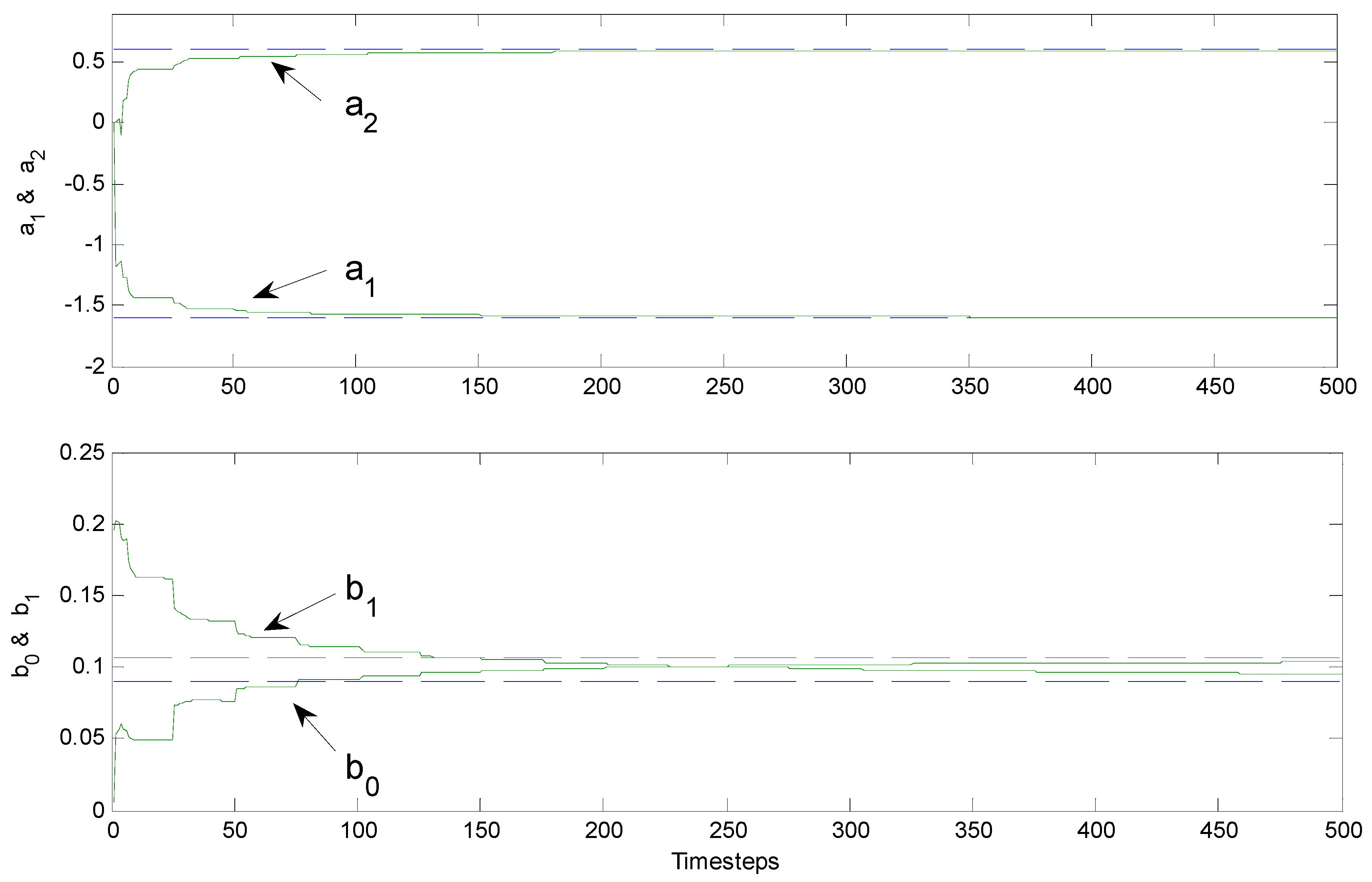
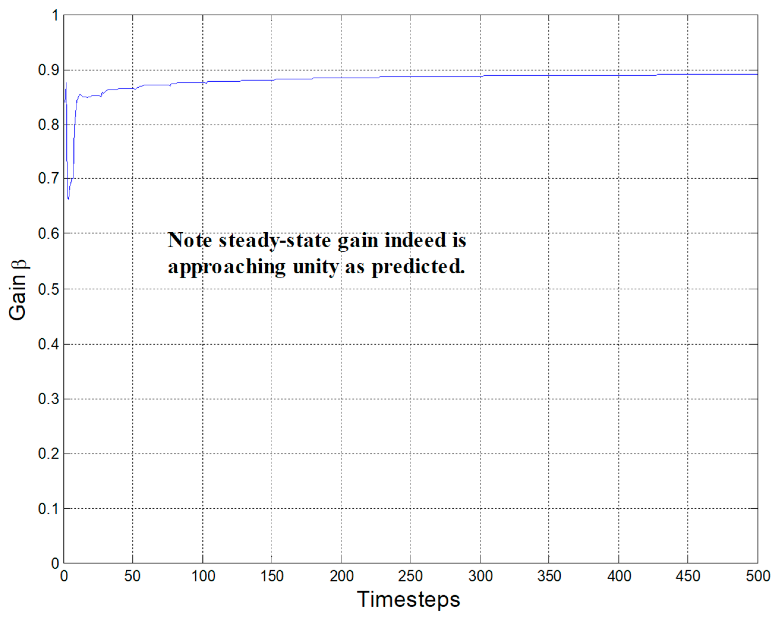
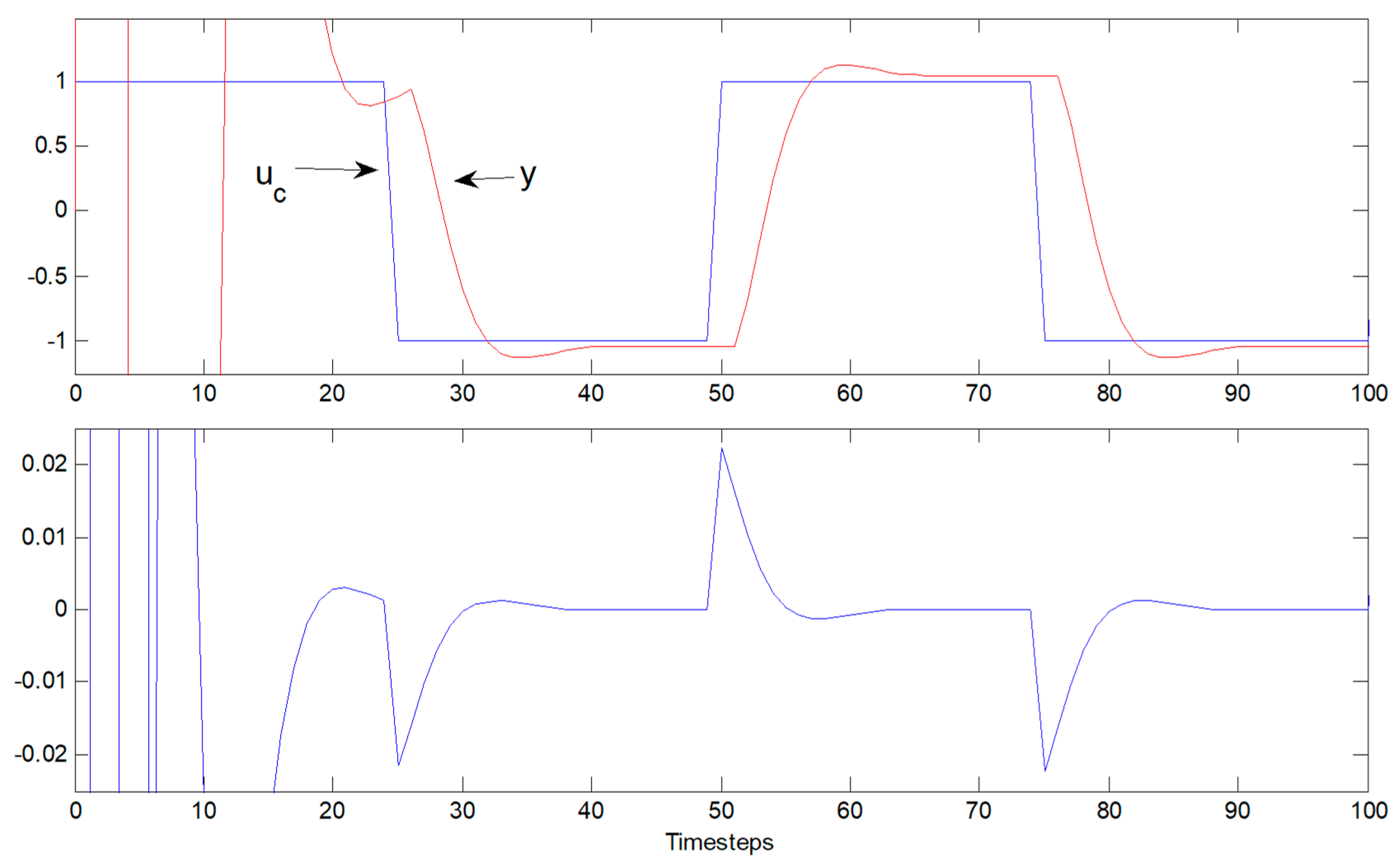
Next, the feedforward control T may be calculated using the following model via [1] (Equation (3.12) on page 95), producing Equation (12). The desired closed-loop is specified in Equation (13) as the plant that generated the data, where Equation (14) results in unity steady-state gain. Also note that no cancellation of system zero is required to achieve this desired closed-loop system. This model satisfied the compatibility conditions (degS < degR; degT < degR) because it has the same pole excess as the process and the process zero is stable (although poorly damped). The min degree (unique) solution to the Diophantine equation results from degR = degAc − degA. From the compatibility condition, it follows that degA0 = 1 (noting this difference from [1]). With no zero cancellation, B+ = 1, and B− = B = b0q + b1. Results following a square wave input are in Figure 3 with parameter identification in Figure 4. Demonstration of steady state unity gain is in Figure 5.
T = βA0 = β(q + a0)
2.2. Non-Minimum Phase Plant Model
Using development identical to that in Section 2.1, we modify the true plant model. Specifically, we change the plant model given in Equation (2) to the non-minimum phase plant in Equation (14).
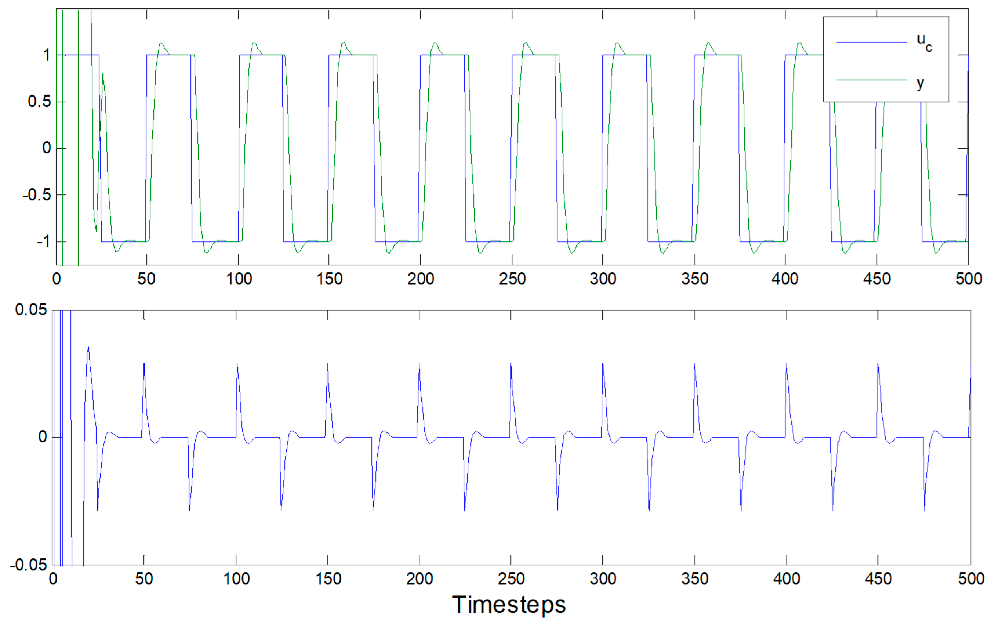
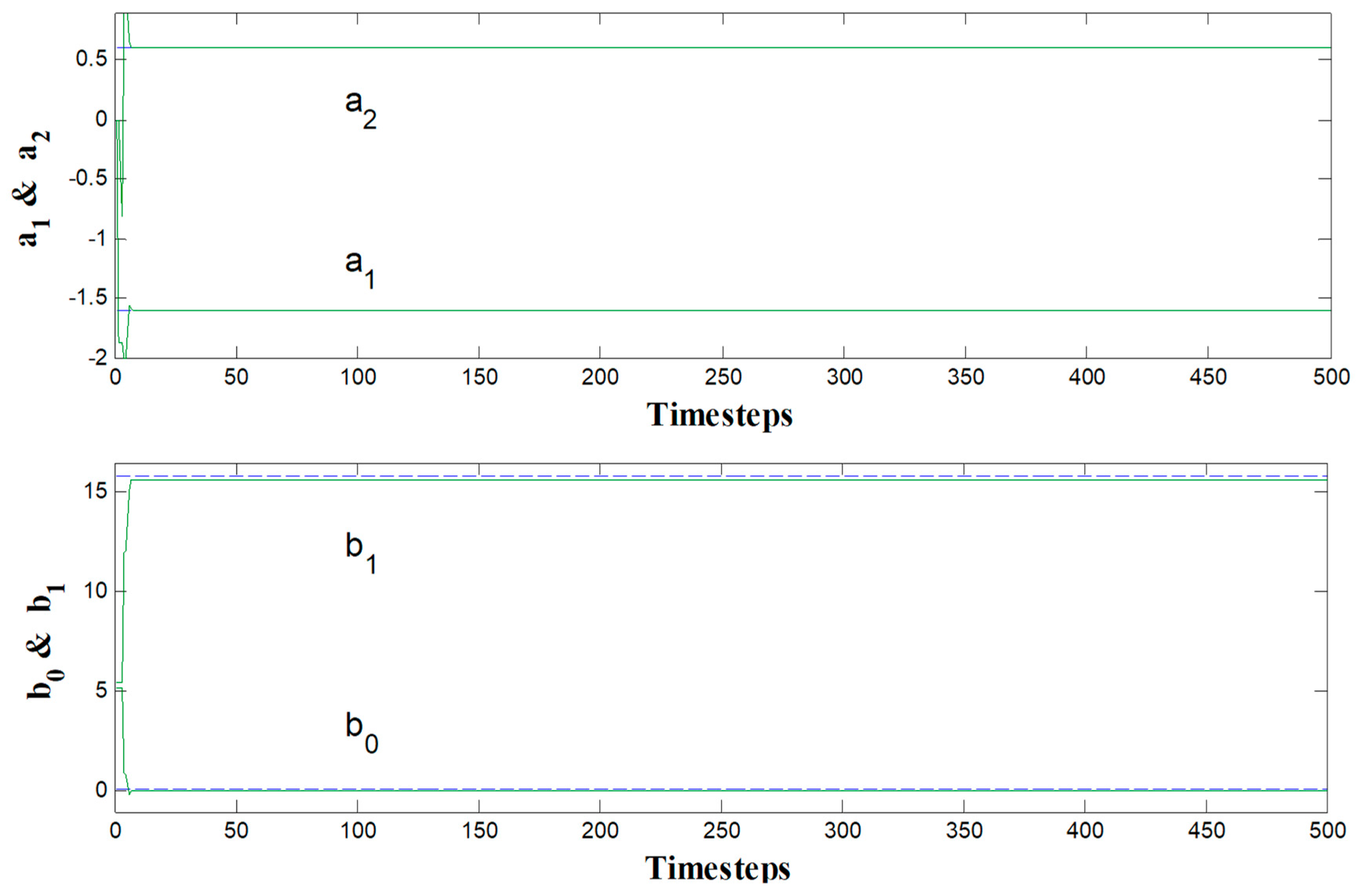
Figure 6 and Figure 7 reveal that the controller effectively controls the plant after an initial startup transient, de-emphasized in the display to emphasize steady state controllability, since the emphasis of this article is the system identification displayed in Figure 8 with the steady-state controllability emphasized in Figure 6 and Figure 7. In particular, notice that the larger error occurring during the transient more quickly forces the parameter estimate convergence in Figure 8.
2.3. Direct Self-Tuner with Increased Plant Pole Excess (d0 = 2)
In the derivation of the direct algorithm, the parameter d0 was the pole excess of the plant. Considering a non-minimum phase system, assume the pole excess is not known.
2.3.1. Modified Plant Model
Direct self-tuners result in extremely simple algorithms as we write control laws directly from the measurements (sacrificing the direct display of plant changes). The model is often parameterized in a manner that is vulnerable to noise amplification. Assuming a linear model in Equation (16) and a desired response according to the model in Equation (17), the process is re-parameterized in terms of the controller starting with the Diophantine equation in Equation (18).
R′ is the term(s) left over after we have factored B+ (Equation (19)). is gain and any term(s) we cannot cancel in Equation (20). A0 implies that it is found by an estimator. Matrix S is the output polynomial of the controller, and Matrix A is the process denominator. This results in Equation (21).
Since R = R′B+, we have R′B = R′B+B− = RB−. This produces an equation with knowns on one side and unknowns on the other side, which we may consider to form a new process model that is parameterized in terms of coefficients of B−, R, and S per Equation (22).
These nonlinear dynamics are simplified by the assumption for non-minimum phase systems that B− = b0 is constant.
2.3.2. Direct Self-Tuning Regulators
In the algorithm, we first use recursive least squares to estimate the coefficients of R and S for the assumed model. For recursive least squares, the input becomes Equation (23). The output becomes Equation (24). We can counter this noise amplification by filtering via an assumed process model in Equation (25).
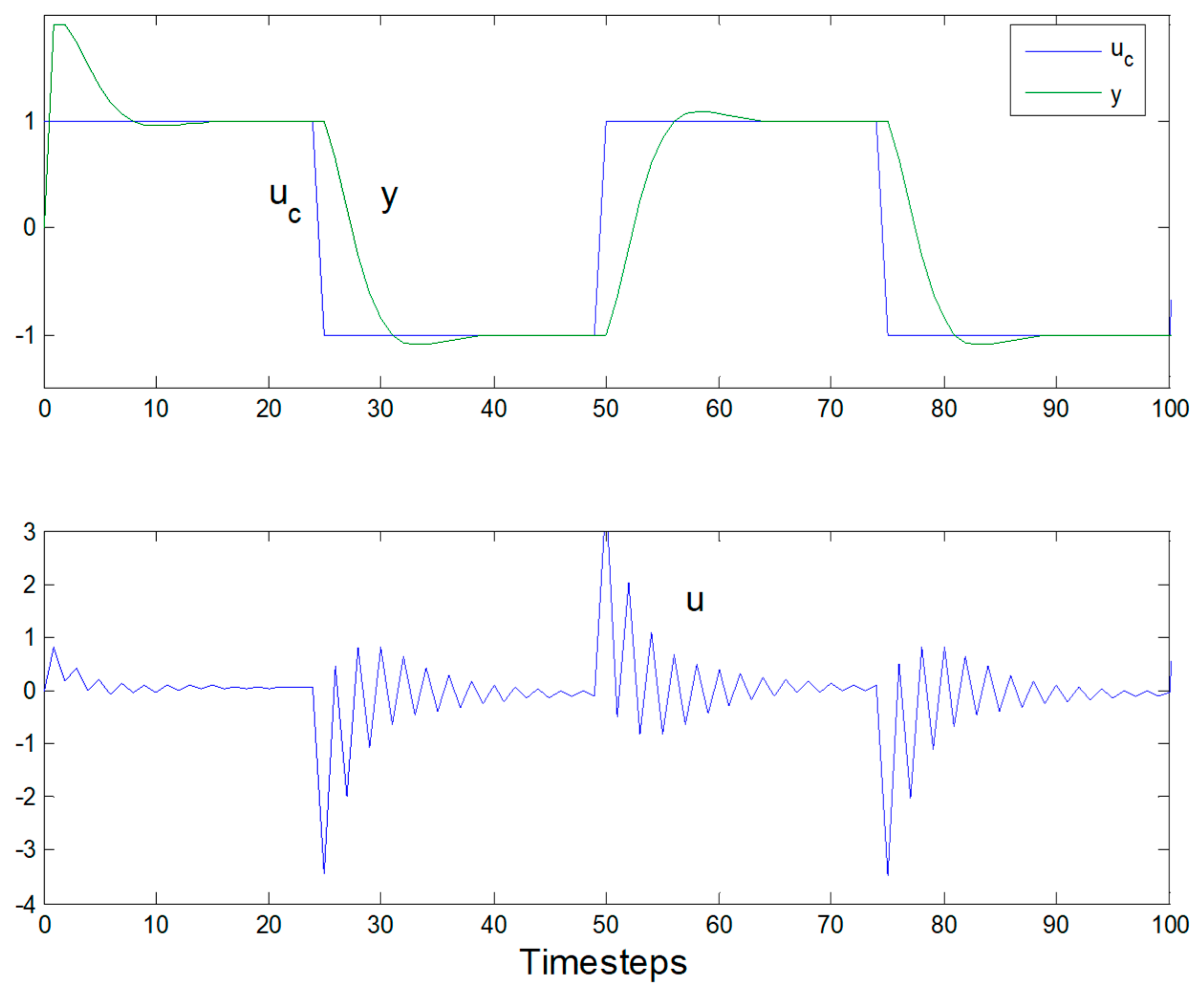
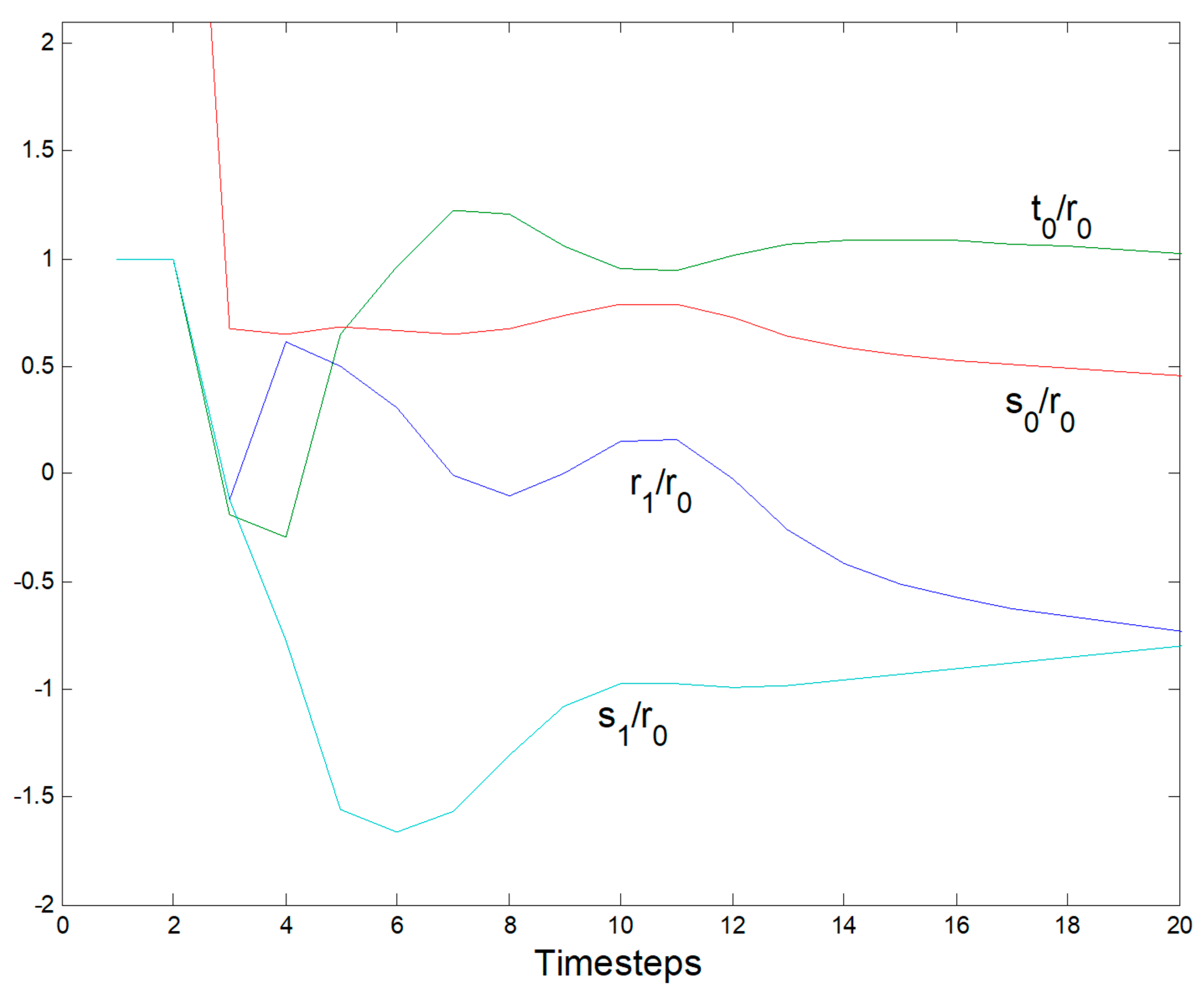
The subscript f denotes filtered signals that are premultiplied by Equation (26) in order to reduce the noise that is generated by the mathematical operation Equation (27) which appears in the denominator. Since our recursive least squares algorithm is estimating control coefficients directly, the algorithm is just that simple! Of particular note is the fact that the algorithm output is dramatically dependent on the initial coefficient guesses. Results following a square wave input are in Figure 9 with pole excess increase in Figure 10 to eliminate control chattering. Normalized parameter estimates are in Figure 11.
3. Brief Discussion of Results
The Diophantine equation was derived for an indirect self-tuner where feedforward and feedback controls were both parameterized in terms of the motor’s math model. As the controller sought to nullify tracking errors, the assumed plant parameters were adapted and quickly converged on the correct parameters of the motor’s math model. Next, a more challenging non-minimum phase system was investigated, and the earlier implemented technique was modified utilizing a direct self-tuner with an increased pole excess. The nominal method experienced control chattering (an undesirable characteristic that could potentially damage the motor during testing), while the increased pole excess eliminated the control chattering, yet maintained effective mathematical system identification. This novel approach permits algorithms normally used for control to instead be used effectively for mathematical system identification.
4. Summary and Conclusions
System identification and system control are closely intertwined [21,22,23,24,25,26,27]. This article begins with a standard problem formulation [2,12,13,14,15,16,17,18,19,20] and ends with very rapid system identification with complementary well-controlled systems. The results here are significant, since system identification of mathematical models is quite often a ubiquitous prerequisite for control engineers. The methods above permit researchers to formulate their problems (including challenging non-minimum phase systems) in such a manner to yield de facto online system identification while maintaining acceptable control even under strenuous trajectory commands (the square wave was used here). Discontinuities present physically unrealizable trajectories to systems being controlled, and the square wave presents repeated time discontinuities.
The methods presented here can use the engineer’s control strategy itself to output the mathematical model of the plant being controlled, and is demonstrated to converge to the correct equation very quickly. In this article, challenging controls with discontinuous steps were utilized to highlight the control recovery from such discontinuities, but also to reveal that they do not degrade parameter convergence, and, therefore, the approach may be generalized to such command inputs (e.g., step, square wave, etc.) without concern for smooth trajectory generation.
The standard problem formulation allows control engineers to account for time-varying systems by simply increasing the forgetting factor that more heavily weights recent inputs, and, furthermore, permits quick implementation of extended least squares and posterior residuals in instances where system bias is suspected.
Conflicts of Interest
The author declares no conflict of interest.
References
- Astrom, K.; Wittenmark, B. Adaptive Control, 2nd ed.; Addison Wesley Longman: Boston, MA, USA, 1995. [Google Scholar]
- Shorey, T.; Tijdeman, R. Exponential Diophantine equations. In Cambridge Tracts in Mathematics; Cambridge University Press: Cambridge, UK, 1986. [Google Scholar]
- Bézout, É. Theorie Generale Des Equations Algebriques (1779); Kessinger Publishing: Whitefish, MT, USA, 2010. [Google Scholar]
- Bhau, D. Brief Notes on the Age and Authenticity of the Works of Aryabhata, Varahamihira, Brahmagupta, Bhattotpala, and Bhaskaracharya. J. R. Asiat. Soc. G. B. Irel. 1865, 1, 392–418. [Google Scholar]
- Schoukens, M.; Noël, J.P. Three Benchmarks Addressing Open Challenges in Nonlinear System Identification. In Proceedings of the 20th World Congress of the International Federation of Automatic Control, Toulouse, France, 9–14 July 2017; pp. 448–453. [Google Scholar]
- Schoukens, M.; Noël, J.P. Wiener-Hammerstein benchmark with process noise. In Proceedings of the Workshop on Nonlinear System Identification Benchmarks, Brussels, Belgium, 25–27 April 2016; pp. 15–19. [Google Scholar]
- Nonlinear System Identification Benchmarks. Available online: http://www.nonlinearbenchmark.org/ (accessed on 28 November 2017).
- Bouc, R. Forced vibration of mechanical systems with hysteresis. In Proceedings of the Fourth Conference on Nonlinear Oscillation, Prague, Czech Republic, 5–9 September 1967; p. 315. [Google Scholar]
- Noël, J.P.; Schoukens, M. Hysteretic benchmark with a dynamic nonlinearity. In Proceedings of the Workshop on Nonlinear System Identification Benchmarks, Brussels, Belgium, 25–27 April 2016; pp. 7–14. [Google Scholar]
- Schoukens, M.; Marconato, A.; Pintelon, R.; Vandersteen, G.; Rolain, Y. Parametric identification of parallel Wiener–Hammerstein systems. Automatica 2015, 51, 111–122. [Google Scholar] [CrossRef]
- Wigren, T.; Schoukens, J. Three free data sets for development and benchmarking in nonlinear system identification. In Proceedings of the 2013 European Control Conference (ECC), Zurich, Switzerland, 17–19 July 2013; pp. 2933–2938. [Google Scholar]
- Sands, T.A. Fine Pointing of Military Spacecraft. Ph.D. Dissertation, Naval Postgraduate School, Monterey, CA, USA, 2007. [Google Scholar]
- Sands, T.; Lorenz, R. Physics-Based Automated Control of Spacecraft. In Proceedings of the AIAA Space Conference & Exposition, Pasadena, CA, USA, 14–17 September 2009. [Google Scholar]
- Sands, T.A. Physics-Based Control Methods. In Advances in Spacecraft Systems and Orbit Determination; InTech Publishers: London, UK, 2012; pp. 29–54. [Google Scholar]
- Nakatani, S.; Sands, T. Simulation of Spacecraft Damage Tolerance and Adaptive Controls. In Proceedings of the IEEE Aerospace Conference, Big Sky, MT, USA, 1–8 March 2014. [Google Scholar] [CrossRef]
- Sands, T. Improved Magnetic Levitation via Online Disturbance Decoupling. Phys. J. 2015, 1, 272–280. [Google Scholar]
- Nakatani, S.; Sands, T. Autonomous Damage Recovery in Space. Int. J. Autom. Control Intell. Syst. 2016, 2, 23–36. [Google Scholar]
- Heidlauf, P.; Cooper, M. Nonlinear Lyapunov Control Improved by an Extended Least Squares Adaptive Feed Forward Controller and Enhanced Luenberger Observer. In Proceedings of the International Conference and Exhibition on Mechanical & Aerospace Engineering, Las Vegas, NV, USA, 2–4 October 2017. [Google Scholar]
- Cooper, M.; Heidlauf, P.; Sands, T. Controlling Chaos—Forced van der Pol Equation. Mathematics 2017, 5, 70. [Google Scholar] [CrossRef]
- Sands, T. Phase Lag Elimination at All Frequencies for Full State Estimation of Spacecraft Attitude. Phys. J. 2017, 3. (accepted). [Google Scholar]
- Ljung, L. System identification. In Signal Analysis and Prediction; Birkhauser: Boston, MA, USA, 1998; pp. 163–173. [Google Scholar]
- Pappalardo, C.M.; Guida, D. Adjoint-based Optimization Procedure for Active Vibration Control of Nonlinear Mechanical Systems. ASME J. Dyn. Syst. Meas. Control 2017, 139, 081010. [Google Scholar] [CrossRef]
- Pappalardo, C.M.; Guida, D. Control of Nonlinear Vibrations using the Adjoint Method. Meccanica 2017, 52, 2503–2526. [Google Scholar] [CrossRef]
- Juang, J.N.; Phan, M.Q. Identification and Control of Mechanical Systems; Cambridge University Press: Cambridge, UK, 2001. [Google Scholar]
- Guida, D.; Nilvetti, F.; Pappalardo, C.M. Parameter Identification of a Two Degrees of Freedom Mechanical System. Int. J. Mech. 2009, 3, 23–30. [Google Scholar]
- Guida, D.; Pappalardo, C.M. Sommerfeld and Mass Parameter Identification of Lubricated Journal Bearing. WSEAS Trans. Appl. Theor. Mech. 2009, 4, 205–214. [Google Scholar]
- Liu, G.P. Nonlinear Identification and Control: A Neural Network Approach; Springer Science & Business Media: Berlin, Germany, 2012; ISBN 978-1-4471-0345-5. [Google Scholar]
Figure 1.
A Wiener–Hammerstein system with process noise: the red blocks represent linear time-invariant dynamics, while the blue block represents a static nonlinearity [7].
Figure 1.
A Wiener–Hammerstein system with process noise: the red blocks represent linear time-invariant dynamics, while the blue block represents a static nonlinearity [7].

Figure 2.
Two-degree (feedforward and feedback) controller topology with commanded control uc and actual control u comprising coefficients R, T, and S, closely following development in [1].
Figure 2.
Two-degree (feedforward and feedback) controller topology with commanded control uc and actual control u comprising coefficients R, T, and S, closely following development in [1].
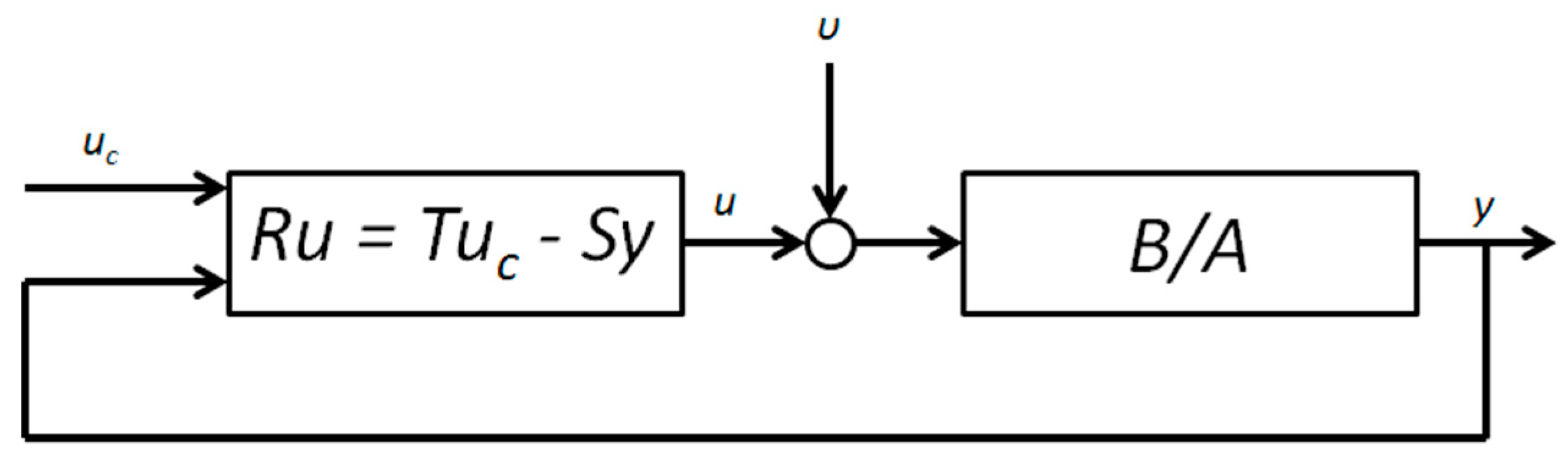
Figure 3.
Control u(t) output y(t) versus time for indirect self-tuner (no zero cancellation) of minimum phase system.
Figure 3.
Control u(t) output y(t) versus time for indirect self-tuner (no zero cancellation) of minimum phase system.
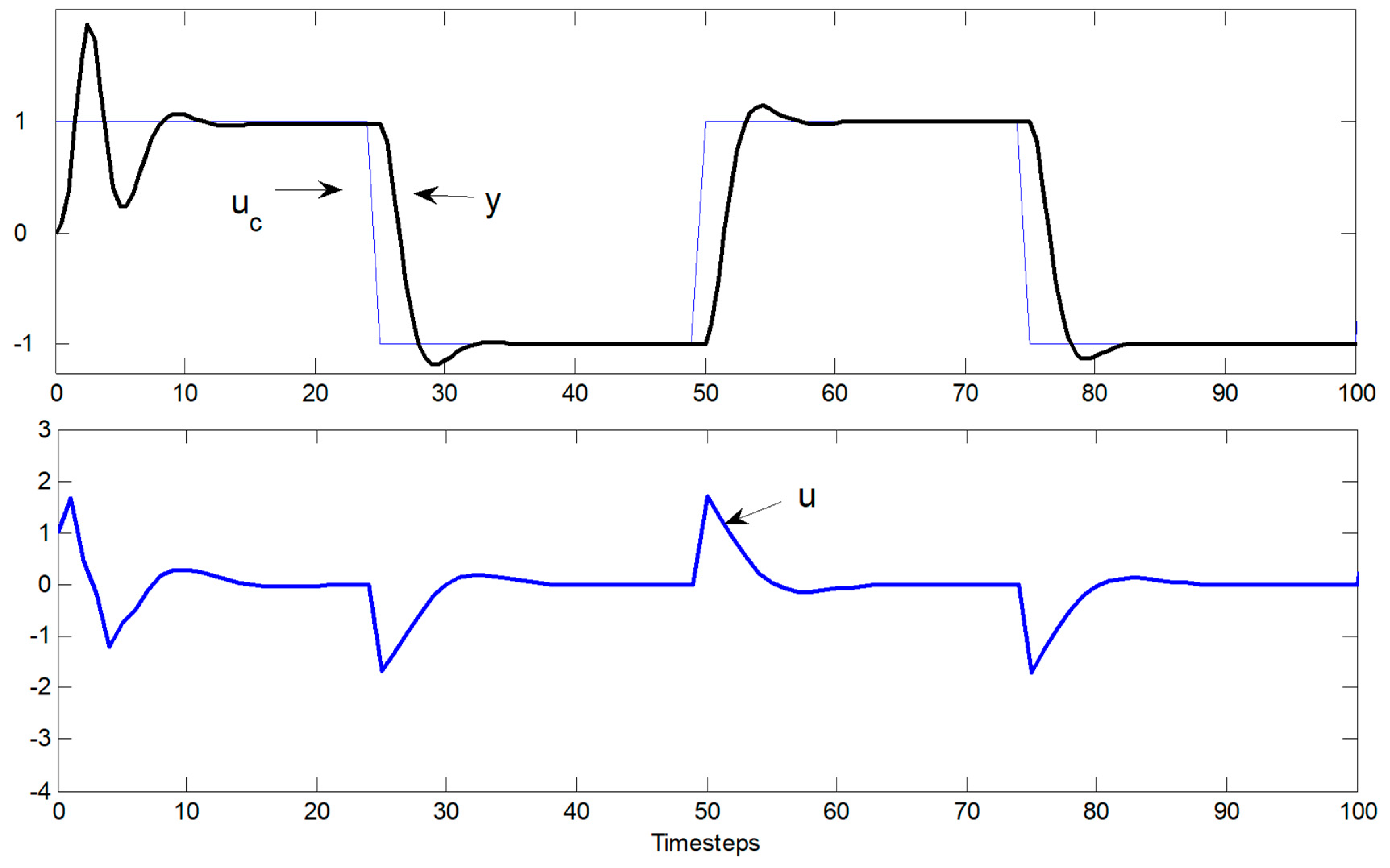
Figure 4.
Parameter identification, indirect self-tuner (without zero cancellation) of minimum phase system.
Figure 4.
Parameter identification, indirect self-tuner (without zero cancellation) of minimum phase system.

Figure 5.
Steady-state gain β of indirect self-tuner (without zero cancellation) of minimum phase system.
Figure 5.
Steady-state gain β of indirect self-tuner (without zero cancellation) of minimum phase system.

Figure 6.
Control u(t) output y(t) versus time for indirect self-tuner (no zero cancellation), non-minimum phase system.
Figure 6.
Control u(t) output y(t) versus time for indirect self-tuner (no zero cancellation), non-minimum phase system.

Figure 7.
Control u(t) output y(t) versus time: time-step propagation extended to 500 to reveal consistent performance following startup transient.
Figure 7.
Control u(t) output y(t) versus time: time-step propagation extended to 500 to reveal consistent performance following startup transient.

Figure 8.
Parameter estimates for non-minimum phase system without zero cancellation.

Figure 9.
Control u(t) output y(t) versus time for Direct Self-Tuner with pole excess d0 = 1: Note the control “chattering”.
Figure 9.
Control u(t) output y(t) versus time for Direct Self-Tuner with pole excess d0 = 1: Note the control “chattering”.

Figure 10.
Control u(t) output y(t) versus time Direct Self-Tuner with increase pole excess d0 = 2: Note elimination of the control “chattering”.
Figure 10.
Control u(t) output y(t) versus time Direct Self-Tuner with increase pole excess d0 = 2: Note elimination of the control “chattering”.
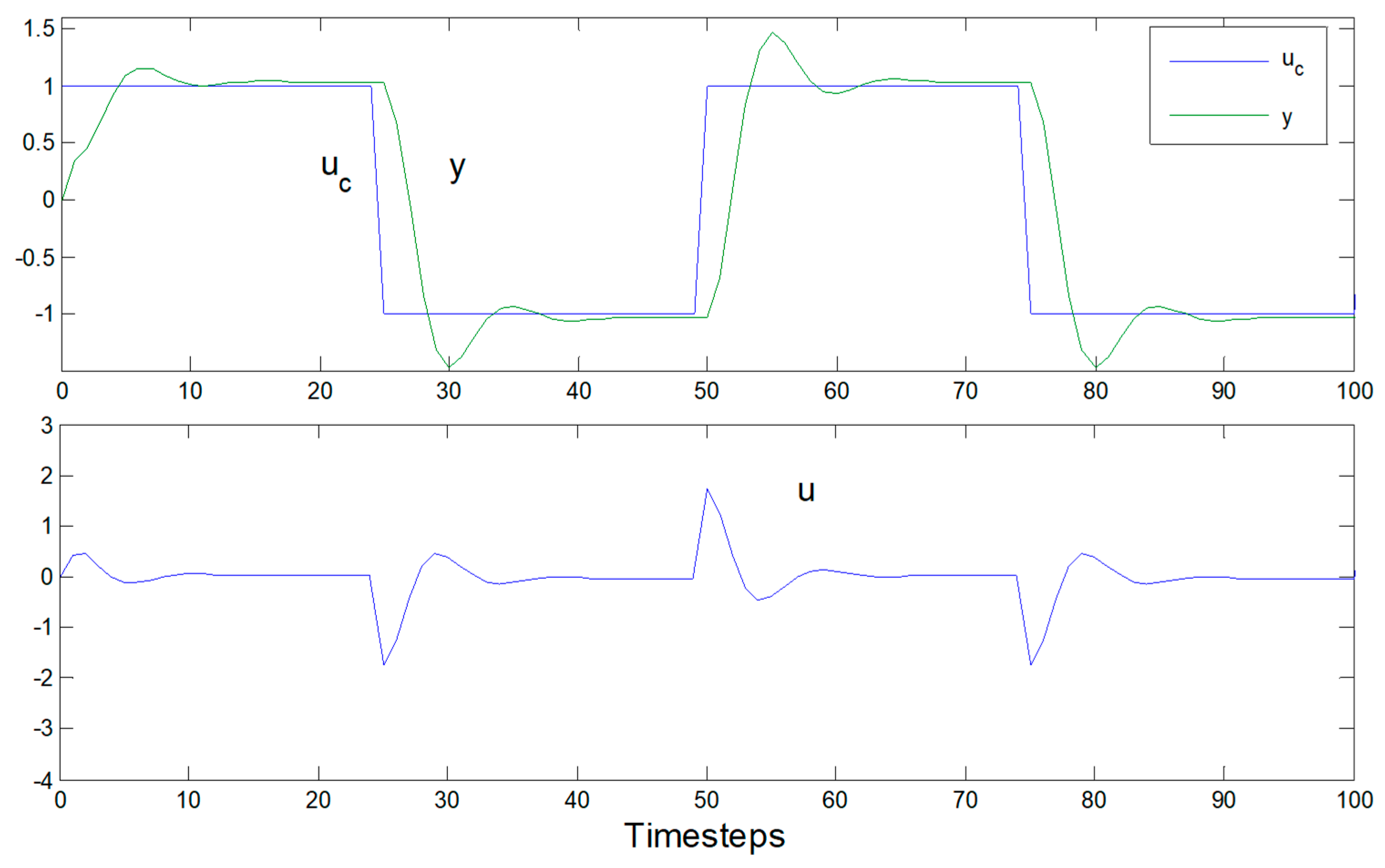
Figure 11.
Normalized parameter estimates: Notice how quickly estimates converge.

© 2017 by the author. Licensee MDPI, Basel, Switzerland. This article is an open access article distributed under the terms and conditions of the Creative Commons Attribution (CC BY) license (http://creativecommons.org/licenses/by/4.0/).
Share and Cite
MDPI and ACS Style
Sands, T. Nonlinear-Adaptive Mathematical System Identification. Computation 2017, 5, 47. https://doi.org/10.3390/computation5040047
AMA Style
Sands T. Nonlinear-Adaptive Mathematical System Identification. Computation. 2017; 5(4):47. https://doi.org/10.3390/computation5040047
Chicago/Turabian StyleSands, Timothy. 2017. "Nonlinear-Adaptive Mathematical System Identification" Computation 5, no. 4: 47. https://doi.org/10.3390/computation5040047
Note that from the first issue of 2016, this journal uses article numbers instead of page numbers. See further details here.