Analysis, Synchronization and Circuit Design of a 4D Hyperchaotic Hyperjerk System
by
 ,
,
Petros A. Daltzis
1, 
Christos K. Volos
2 ,
,
Hector E. Nistazakis
1,*, 
Andreas D. Tsigopoulos
3 and
George S. Tombras
1 1
Department of Electronics, Computers, Telecommunications and Control, Faculty of Physics, National and Kapodistrian University of Athens, GR-157 84 Athens, Greece
2
Laboratory of Nonlinear Systems—Circuits & Complexity, Department of Physics, Aristotle University of Thessaloniki, GR-541 24 Thessaloniki, Greece
3
Department of Battle Systems, Naval Operations, Sea Studies, Navigation, Electronics and Telecommunications, Hellenic Naval Academy, Hadjikyriakou Ave., GR-185 39 Piraerus, Greece
*
Author to whom correspondence should be addressed.
Computation 2018, 6(1), 14; https://doi.org/10.3390/computation6010014
Submission received: 15 December 2017
/
Revised: 31 January 2018
/
Accepted: 2 February 2018
/
Published: 6 February 2018
(This article belongs to the Special Issue Selected Papers from the 7th International Conference on Experiments/Process/System Modeling/Simulation/Optimization (IC-EPSMSO 2017))
Abstract
:In this work, a 4D hyperchaotic hyperjerk system, with better results for its Lyapunov exponents and Kaplan–Yorke dimension regarding other systems of this family, as well as its circuit implementation, is presented. Hyperchaotic hyperjerk systems depict complex dynamical behavior in a high-dimensional phase space with n ≥ 4, offering robustness against many types of attacks in private communications. For this reason, an adaptive controller in order to achieve global chaos synchronization of coupled 4D hyperchaotic hyperjerk systems with unknown parameters is designed. The adaptive results in this work are proved using Lyapunov stability theory and the effectiveness of the proposed synchronization scheme is confirmed through the simulation results.
1. Introduction
Nonlinear dissipative dynamical systems characterized by high sensitivity on initial conditions are known today as chaotic systems. The aforementioned feature of sensitivity, which is present in these kinds of dynamical systems, causes the trajectories of two identical chaotic systems to divert exponentially, despite the almost identical initial conditions.
It is known from literature that a hyperchaotic system is defined as a dynamical system with at least two positive Lyapunov exponents. As a consequence, the dynamics of a system like that can expand in several different directions simultaneously. It is well known that the minimum dimension for an autonomous, continuous-time, hyperchaotic system is four. Since the discovery of a first 4D hyperchaotic system by Rössler in 1979 [1], many 4D hyperchaotic systems have been reported in literature, such as the hyperchaotic Lorenz system [2], the hyperchaotic Lü system [3], the hyperchaotic Chen system [4], the hyperchaotic Wang system [5], the hyperchaotic Newton–Leipnik system [6], the hyperchaotic Jia system [7], the hyperchaotic Vaidyanathan system [8], etc.
In mechanics, if the scalar x(t) represents the position of a moving object at time t, then the first derivative, , represents the velocity, the second derivative, , represents the acceleration and the third derivative, , represents the jerk or jolt [9]. In mechanics, a jerk system is described by an explicit third order ordinary differential equation describing the time evolution of a single scalar variable x according to the dynamics:
A particularly simple example of a jerk system is the famous Coullet system [10] given by
where g(x) is a nonlinear function such as g(x) = b(x2 − 1), which exhibits chaos for a = 0.6 and b = 0.58.
A generalization of the jerk dynamics is given by the dynamics
An ordinary differential equation of the Formula (3) is called a hyperjerk system since it involves time derivatives of a jerk function [11].
Due to the importance of enabling a chaotic or hyperchaotic system to maintain a desirable dynamical behavior, many relative techniques have been proposed describing either a static or a dynamic feedback control, or an open-loop control method. In some contemporary cases, the problem that must be solved is the investigation of a state feedback control law in order to stabilize the system around its unstable equilibrium point [12,13]. Some popular techniques in literature are the active control method [14,15], the adaptive control method [16,17,18], the sampled data feedback control method [19,20], the time delay feedback approach [21,22], the backstepping method [23,24], the sliding mode control method [25,26], the fuzzy-model-based control method [27] and the Ott, Grebogy and Yorke (OGY) method [12].
The study of chaos in the last decades had a tremendous impact on the foundations of science and engineering, and one of the most recent exciting developments in this regard is the discovery of chaos synchronization. Therefore, the methods used for controlling nonlinear systems can also be applied for synchronizing two or more coupled chaotic oscillators. Some of the aforementioned methods only apply to chaotic systems while others need several controllers to realize synchronization, focusing on the condition with unknown parameters and disturbances [28,29]. Synchronization of coupled chaotic systems is defined as the phenomenon that occurs when a chaotic system drives another chaotic system by adjusting a given property of their motion. Due to the feature of exponential divergence of trajectories of two identical chaotic systems, which start with nearly the same initial conditions, the synchronization of chaotic systems is an interesting research topic in chaos literature. In addition, synchronized chaotic systems can then set up private communication systems with applications in secure communications [30,31,32,33,34], cryptosystems [35,36] and encryption [37,38], offering robustness against various attack methods.
Yamada and Fujisaka [39] conducted the first research on synchronizing a chaotic system, while Pecora and Carroll [40,41] discovered that chaotic systems can be synchronized when an appropriate coupling design is found, such as that the chaotic time evolutions of the two systems become identical. Other approaches regarding the synchronization of chaotic systems are either by the use of state observers or by the use of control laws according to the Lyapunov stability theory. The main types of synchronization are the complete synchronization [42,43], the phase synchronization [44,45], the generalized synchronization [46,47], the antisynchronization (AS) [48,49], the generalized projective synchronization [50] and the hybrid synchronization [51].
Especially in the case of complete synchronization, the main aim is to use the output of the master system in order to control the slave system. In this way, the output of the slave system tracks the output of the master system asymptotically with time. For the aforementioned control methods, adaptive control is the main method, which is used when some or all of the chaotic or hyperchaotic system’s parameters are not available for measurement and estimates the uncertain parameters of the systems [16,52].
In this research work, a 4D hyperjerk system with hyperchaotic behavior is studied, by using some of the most used tools of nonlinear dynamics, such as bifurcation diagrams, Lyapunov exponents, phase portraits and Poincaré maps. In addition, the circuit of the proposed dynamical system, which proves its feasibility, is designed. Furthermore, an adaptive synchronization scheme for a system of coupled 4D hyperchaotic hyperjerk systems has been developed. For the obtained, with this method, main adaptive results are proved using Lyapunov stability theory. The effectiveness of the synchronization scheme, which is used in this work, has proved through the simulation results.
The rest of the paper is organized as follows. The next section provides a brief description of the 4D hyperchaotic hyperjerk system. Section 3 presents the analysis of the proposed system’s dynamics. The circuit realization of the 4D hyperchaotic hyperjerk system is discussed in Section 4. The adaptive synchronization scheme for a system of two coupled 4D hyperchaotic hyperjerk systems is presented in Section 5. Finally, Section 6 outlines the main points that have been reached with this research study.
2. Description of the 4D Hyperchaotic Hyperjerk System
2.1. Model of the 4D Hyperjerk System
In 2006, Chlouverakis and Sprott [53] discovered a simple hyperchaotic hyperjerk system given by the dynamics
which can also be expressed as the following system (5) of differential equations:
The aforementioned hyperjerk system has only one nonlinearity and when A = 3.6 it exhibits hyperchaotic behavior with Lyapunov exponents: L1 = 0.132, L2 = 0.035, L3 = 0 and L4 = −1.250. For these values of Lyapunov exponents, the Kaplan–Yorke dimension [54,55,56] of the hyperjerk system (5) is defined as:
where L1 ≥ ... ≥ Lj are the Lyapunov exponents of the chaotic system and j is the largest integer for which L1 + L2 + ... + Lj ≥ 0. Thus, the Kaplan–Yorke dimension of the hyperjerk system (5) is easily calculated as DKY = 3.13.
Later, Daltzis et al. [57] presented a new 4D hyperjerk system (7), which is based on system (4), in which one more nonlinearity, viz. the absolute nonlinearity (), has been added:
System (7), when selecting a = 3.7, b = 0.1 and c = 1.5 and initial conditions (x1(0), x2(0), x3(0), x4(0)) = (0.1, 0.1, 0.1, 0.1), has Lyapunov exponents as: L1 = 0.1555, L2 = 0.0330, L3 = 0 and L4 = −1.6100, while the Kaplan–Yorke dimension of system (7) is DKY = 3.1171. Thus, system (7) is also a hyperchaotic 4D hyperjerk system.
In this work, a 4D hyperjerk system by replacing the absolute nonlinearity () with () to system (7) and with a slightly different set of values for the system parameters is studied. Thus, the new 4D hyperjerk system is given in system form as:
where a, b and c are positive parameters. In this paper, we shall show that system (8) is hyperchaotic when the parameters a, b and c take the values a = 3.8, b = 0.1 and c = 1.5.
For these parameter values, the Lyapunov exponents of the hyperjerk system (8), which are calculated in this work by using Wolf’s algorithm [58] are obtained as: L1 = 0.1909, L2 = 0.06462, L3 = 0 and L4 = −1.81846. It is easily seen that the maximal Lyapunov exponent (MLE) of our novel hyperchaotic hyperjerk system (8) is L1 = 0.1809, which is greater than the respective MLE of systems (5) and (7). In addition, the Kaplan–Yorke dimension of the novel hyperjerk system (8), has been calculated as: DKY = 3.1405. Thus, the Kaplan–Yorke is also greater than the respective DKY of hyperjerk systems (5) and (7). This shows that the proposed hyperchaotic 4D hyperjerk system (8) exhibits more complex behavior than systems (5) and (7). Furthermore, the proposed in this work system has better results concerning others reported in literature hyperchaotic hyperjerk systems concerning their MLE and only one (see Ref. [59]) has greater Kaplan–Yorke dimensions (see Table 1). Therefore, the high-dimensional phase space of the proposed hyperjerk system combined with its high Kaplan–Yorke dimension, especially in regard to the other reported systems, guarantees the system’s complex dynamical behavior, which contributes to the required robustness.
In Figure 1, the hyperchaotic phase portraits of the proposed hyperjerk system (8) are illustrated. In more details, six different phase portraits, which are produced from the combinations of the four variables x1–x4, show the system’s strange attractor for the selected set of parameters and initial conditions. Furthermore, in Figure 2, the Poincaré maps, which are produced by selecting two different planes, display the system (8)’s strange attractor. The study of continuous dynamical systems, like the proposed system (8), through a Poincaré map is one of the most popular topics in nonlinear dynamical analysis. This is done by taking intersections of the system’s orbit into the plane x2 = 0 with dx3/dt > 0. Naturally, for a n dimensional attractor, the Poincaré map gives rise to (n − 1) points, which can describe the dynamics of the attractor properly. Thus, this is an artificial way of reducing the map by dropping its dimension. In this direction, the organized set of points in the Poincaré maps of Figure 2 is an indication of system’s chaotic behavior, while the discrete number of n points is an indication of periodic state of period-n. Finally, a closed curve in the Poincaré map is an indication of the system’s quasiperiodic behavior.
2.2. Equilibrium Point Analysis
The 4D hyperchaotic hyperjerk system (8) has only one equilibrium point E(0, 0, 0, 0) and the Jacobian matrix, by linearizing the system at the equilibrium point E, is expressed as:
Thus, system (8), at the equilibrium point E, has a characteristic equation, which can described as:
By using system (8)’s characteristic Equation (10), we can find the stability of the equilibrium point E. It is obvious that the stability of system’s equilibrium point E(0, 0, 0, 0) depends only on the parameters a, b. Therefore, by choosing a = 3.8 and b = 0.1, we find the eigenvalues as: λ1 = 0.16385 + 1.89874i, λ2 = 0.16385 − 1.89874i, λ3 = −0.16385 + 0.498477i and λ4 = −0.16385 − 0.498477i. Based on the theory, according to the aforementioned eigenvalues, equilibrium point E is unstable.
2.3. Dissipativity and Invariance
It is also known from the theory that by using the general condition of dissipativity into the proposed system (8), we can find that
Therefore, system (8) is obviously dissipative for c > 0.
In addition, system (8)’s invariance is indicated by the coordinate transformation (x1, x2, x3, x4) → (−x1, −x2, −x3, x4). Therefore, (−x1, −x2, −x3, x4) is also a solution for the same values of parameters a, b, c and the system can display symmetric attractors.
3. Analysis of the 4D Hyperjerk Dynamics
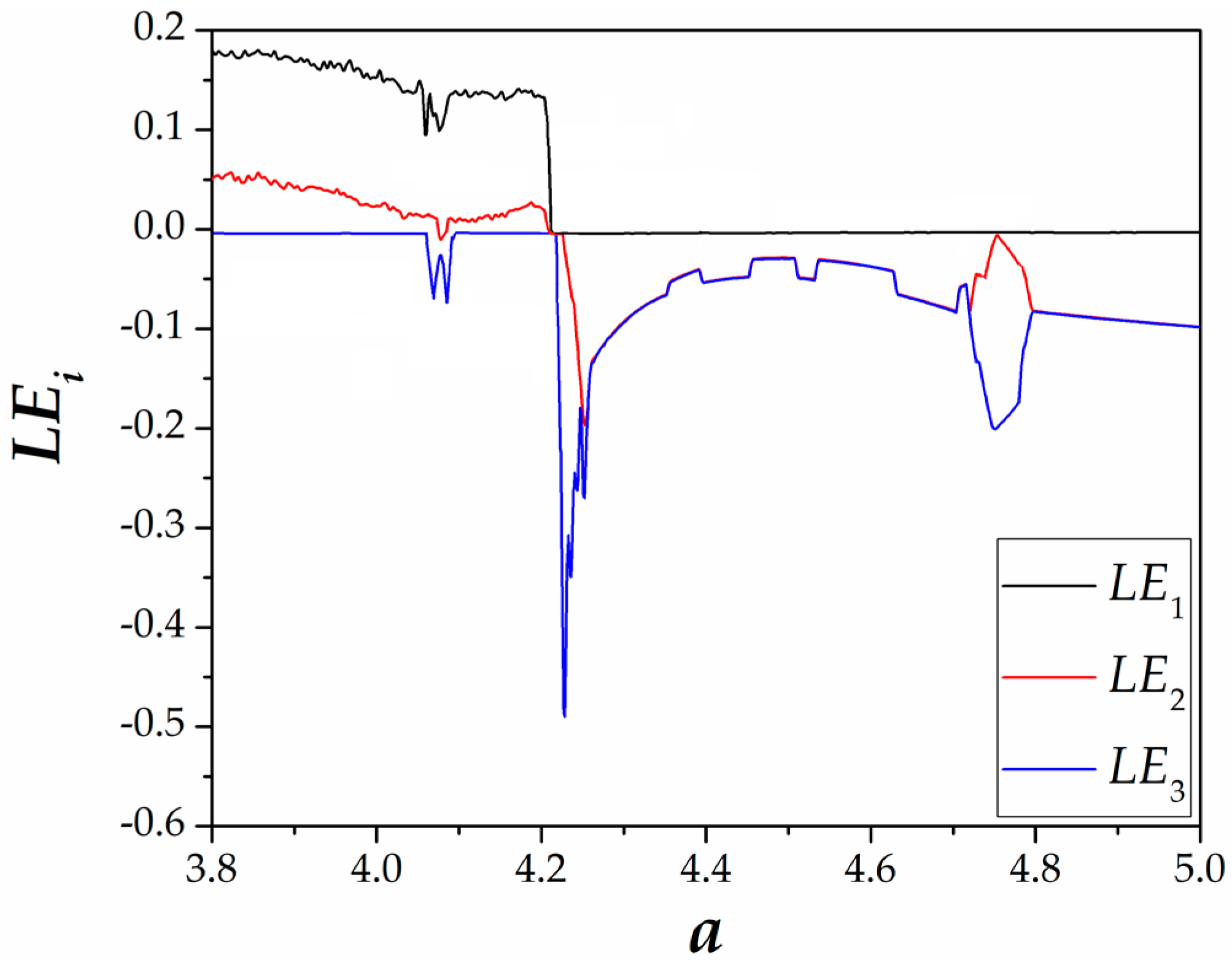
Next, the investigation of the effect of parameter a on system’s dynamics is presented. Due to the fact that the values of parameters b, c do not affect the system’s dynamics but only the size of the attractors, the study of the effect of the parameters b, c has been ignored in this work. The bifurcation diagram and the spectrum of the system’s three largest Lyapunov exponents, by varying the value of the bifurcation parameter a in the range from 3.8 to 5, are presented in Figure 3 and Figure 4, respectively.
The bifurcation diagram is a very important tool in nonlinear theory, as it provides an overview of the system’s behavior in a range of values of a critical parameter, which is called a bifurcation parameter. These diagrams are produced with repetitive depictions by altering the bifurcation parameter with a small step. Therefore, similar to the Poincaré map, the discrete number of n points in the bifurcation diagram is an indication of periodic state of period-n, while a region with an infinite number of points is an indication of the system’s chaotic behavior. For the production of the bifurcation diagram of Figure 3, we have chosen as the trajectory’s cutting plane the x2 = 0 with dx3/dt > 0, while the parameter a increases with very small step. In addition, the initial conditions at each iteration are (x1(0), x2(0), x3(0), x4(0)) = (0.1, 0.1, 0.1, 0.1).
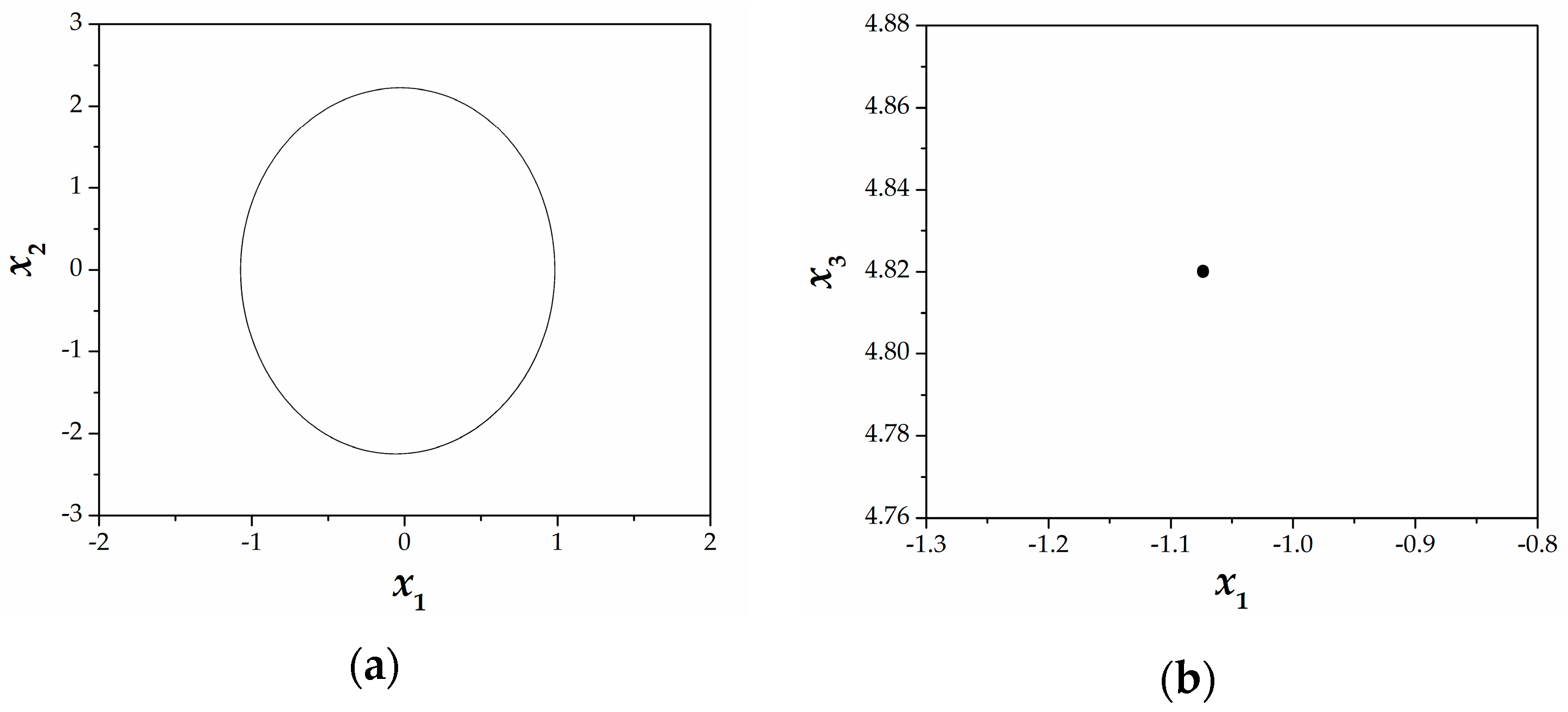
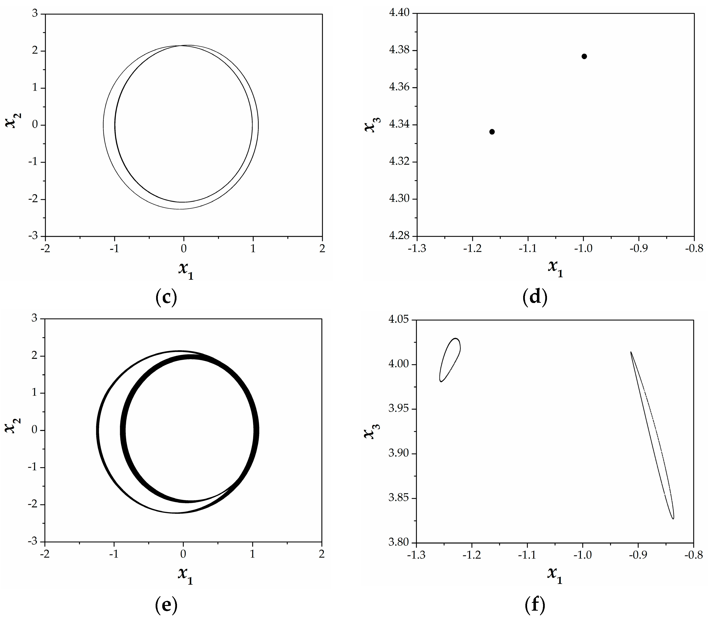
A route to chaos through a quasiperiodic behavior, when decreasing the value of a, is observed in the bifurcation diagram of Figure 3. In more detail, the proposed system (8) displays periodic behavior for a ≥ 4.21, (period-1 steady state and period-2 steady state), which is confirmed from the phase portraits of Figure 5a,c and Poincaré maps of Figure 5b,d, respectively. Especially in the Poincaré maps, which are produced with the same technique as described for the production of the bifurcation diagram, a discrete number of points showing the period of system (8) are depicted. As the parameter a further decreases, the system through a quasiperiodic behavior, which appears in a very narrow band (4.207 ≤ a < 4.210), is driven to a complex behavior for a < 4.207 (Figure 5e). System (8)’s quasiperiodic behavior is confirmed from the closed curves in the Poincaré map of Figure 5f, according to the theory. In addition, the system’s complex behavior for a < 4.207 is mainly hyperchaotic, except for a narrow band in which the system’s behavior is chaotic. The diagram of the spectrum of the three largest Lyapunov exponents of Figure 4 confirms the system’s hyperchaotic behavior due to the fact that, in the aforementioned region (a < 4.207), the system has two positive Lyapunov exponents.
4. Circuit Realization of the Proposed System
The physical realization of theoretical chaotic models through the design of electronic circuits is the classical approach for the verification of their feasibility. Furthermore, the aforementioned approach has been applied in a large number of chaotic systems’ engineering applications, such as true and pseudo random bit generation [63,64,65,66,67], chaotic video communication scheme via a wide area network (WAN) remote transmission [68], audio encryption scheme [69], autonomous mobile robots [70], chaotic communication systems [71], image encryption [72,73,74,75], etc. For this reason, analog and digital approaches have been applied to realize chaotic oscillators by using different kinds of electronic devices such as common off-the-shelf electronic components [76,77], integrated circuit technology [78,79], microcontroller [80] or field-programmable gate array (FPGA) [81,82,83].
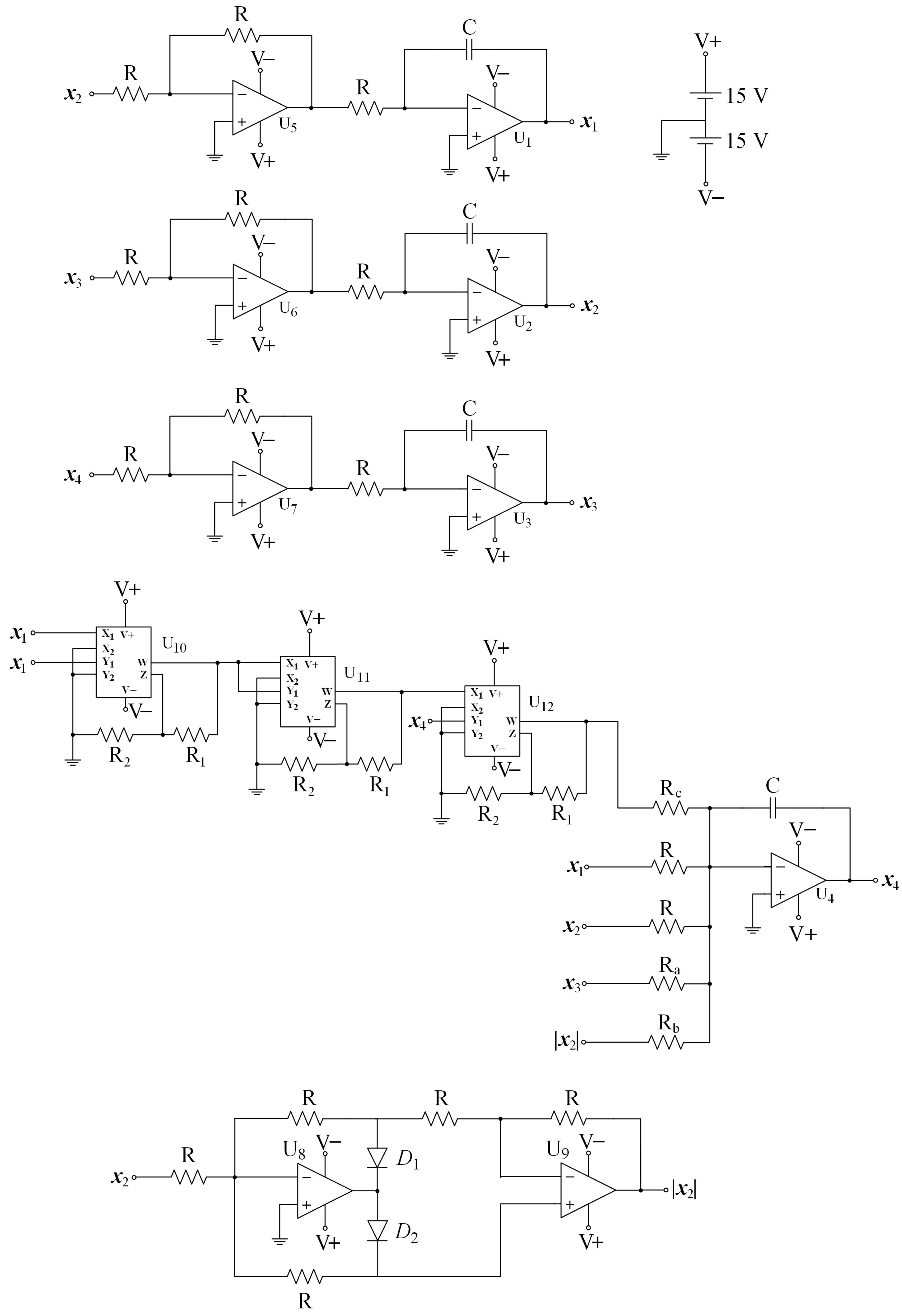
Therefore, in this section, the circuit implementation of the proposed hyperjerk system (8) is presented. In more detail, Figure 6 depicts the circuit that has been designed by using twenty-five resistors, four capacitors, nine operational amplifiers and three analog multipliers (AD633). Four of the operational amplifiers (U1–U4) are configured as Resistor-Capacitor integrators, which is an important operation required in the derivation of the equivalent electronic circuit. The specific realization of the RC integrators, which are very well known in literature, exploits the properties of the operational amplifiers in the linear region, producing in general a current , where VC is the voltage accross the capacitor. Other three operational amplifiers have been used as inverting amplifiers (U5–U7), which use negative feedback to amplify the input voltage. The last ones (U8, U9) with the two diodes (1N4007) are used for implementing the absolute nonlinearity (). The selected configuration for the absolute nonlinearity gives the best results according to literature. Furthermore, the three multipliers (U10–U12) are used for implementing the quintic term c . The low-cost analog multipliers AD633, which are used for this purpose, is the most common approach for realizing polynomial terms or products, like the quintic term cx4x1.
With the use of Kirchhoff’s circuit laws into the proposed circuit of Figure 6, we derive the mathematical model of the hyperjerk system, which is described by the following equations:
where x1, x2, x3 and x4 correspond to the voltages on the integrators (U1–U4), respectively, while the power supply is ±15 V. System (12) is normalized by using τ = t/RC. It can thus be suggested that system (12) is equivalent to system (8) with a = R/Ra, b = R/Rb and c = R/RC. The values of circuit components are R = 100 kΩ, R1 = 10 kΩ, R2 = 90 kΩ, Rb = 1 MΩ, Rc = 66.666 kΩ, and C = 1 nF. In order to change the parameter a, a variable resistor Ra can be used.
The designed circuit of Figure 6 has been implemented by using the well-known Multisim program. In this way, PSpice results of the phase portraits in various planes are reported in Figure 7. It is easy to see the good agreement between system (8)’s numerical results (Figure 1) and the circuit’s simulation results (Figure 7).
5. Synchronization Scheme
As it has been mentioned, the synchronization of chaotic systems is an interesting research topic in literature due to its applications in secure communication schemes and cryptosystems. In order to study the possibility of synchronization of two coupled identical 4D hyperchaotic hyperjerk systems with an unknown system’s parameters, an adaptive control law has been used. The adaptive control is the main method, which is used when some or all the system parameters are not available for measurement and estimates for the uncertain parameters of the systems [16,52]. Therefore, it could be useful in the aforementioned applications.
Therefore, in this work, as the master system, the proposed 4D hypechaotic hyperjerk system (8) is used, while the slave system is given by the following system dynamics:
where yi, (i = 1, ..., 4) are the states and ui, (i = 1, ..., 4) are the adaptive controls to be determined. As it is mentioned, the parameters a, b, c, in systems (8) and (13) are unknown and the design goal is to find adaptive feedback controls ui that uses estimates for the parameters a, b, c, respectively, so as to render the states of the systems (8) and (13) fully synchronized asymptotically.
The synchronization error between the chaotic systems (8) and (13) is defined as:
Thus, the synchronization error dynamics is given by the following equations:
We take the adaptive control laws defined by
where ki, (i = 1, ..., 4) are positive gain constants and are the parameter update laws.
Substituting Label (16) into Label (15), we obtain the closed-loop error dynamics as:
As parameters’ estimation errors, we used the equations:
By differentiating Equations (18) with respect to t, we can obtain
Therefore, by using Equations (18), we can rewrite the closed-loop system (18) as:
Next, the following quadratic Lyapunov function is used:
By differentiating the quadratic Lyapunov function V of Equation (22) along the trajectories of the systems (21) and (20), we obtain the following:
Therefore, the following parameter update laws we have taken are:
Next, we establish the main results of this section.
Theorem 1.
The 4D hyperchaotic hyperjerk systems (8) and (13) with unknown parameters are globally and exponentially synchronized for all initial conditions by the adaptive feedback control law (16) and the parameter update laws (23), where ki, (i = 1, ..., 4) are positive constants.
Proof.
We prove the aforementioned theorem by using the Lyapunov stability theory. For this reason, the quadratic Lyapunov function V of Equation (21), which is positive definite on R7, is used. Therefore, the time derivative of V, by substituting the parameter update laws (23) into (22) is obtained as:
From Equation (24), it is clear that is a negative semi-definite function on R7. In addition, it is concluded that the synchronization error vector e(t) = (e1(t), e2(t), e3(t), e4(t)) and the parameter estimation error (ea(t), eb(t), ec(t)) are globally bounded.
By defining k = min(k1, k2, k3, k4), then it follows from Equation (24) that
Thus,
By integrating the inequality (26) from 0 to t, we have taken:
Therefore, from Equation (27), it follows that , while from system (16), it can be deduced that . Thus, we can conclude that for all initial conditions e(t) → 0 exponentially as t → ∞, by using the Barbalat’s lemma [84].
This completes the proof. ☐
As in Section 3, the classical fourth-order Runge–Kutta method is used in order to solve the system of differential Equations (8), (13) and (23), when the adaptive control laws (16) are applied. In addition, the same parameter values of the 4D hyperjerk systems (8) and (13) as in the hyperchaotic case of Section 2 are used, while the gain constants are taken as ki = 10, for i = 1, 2, 3, 4.
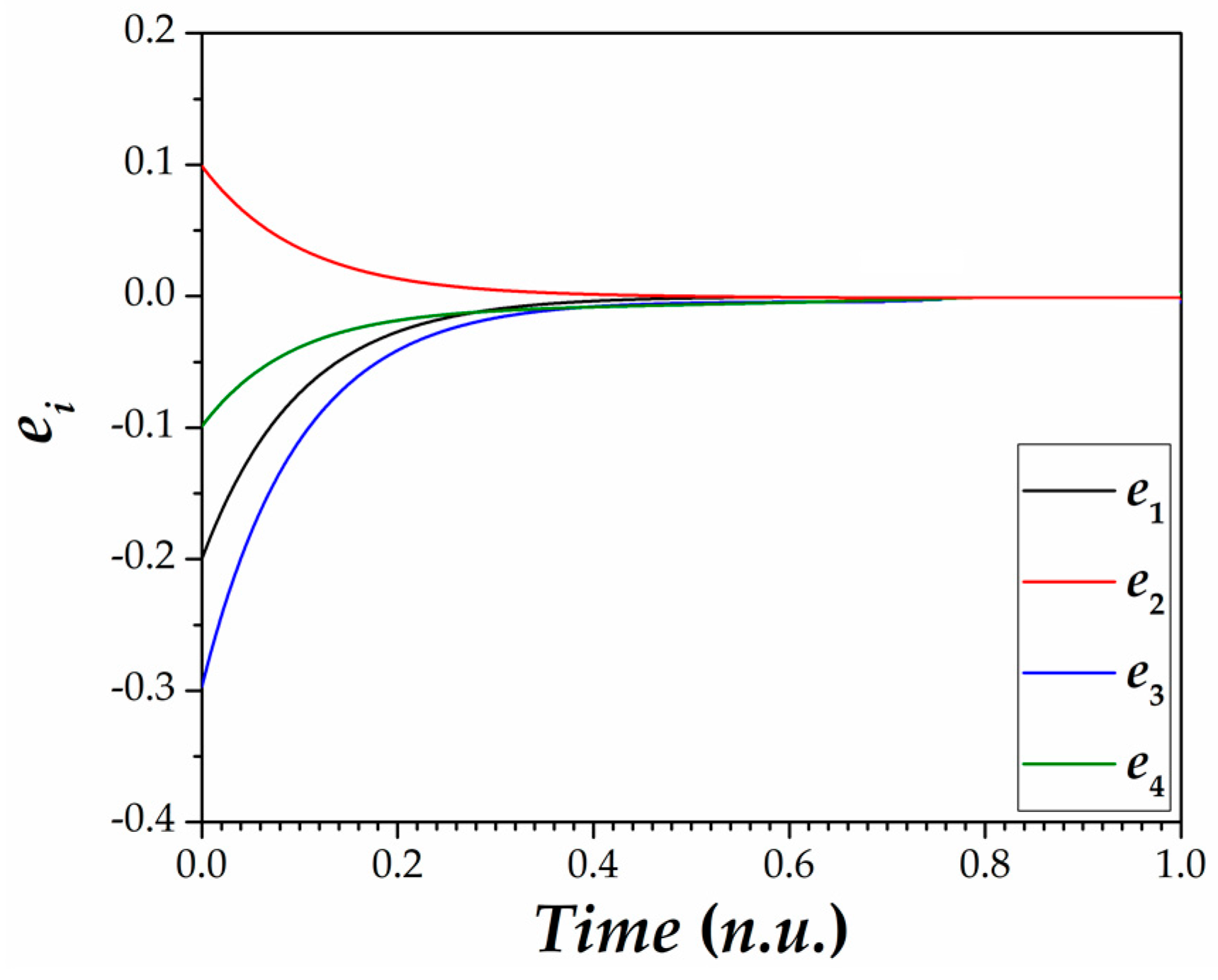
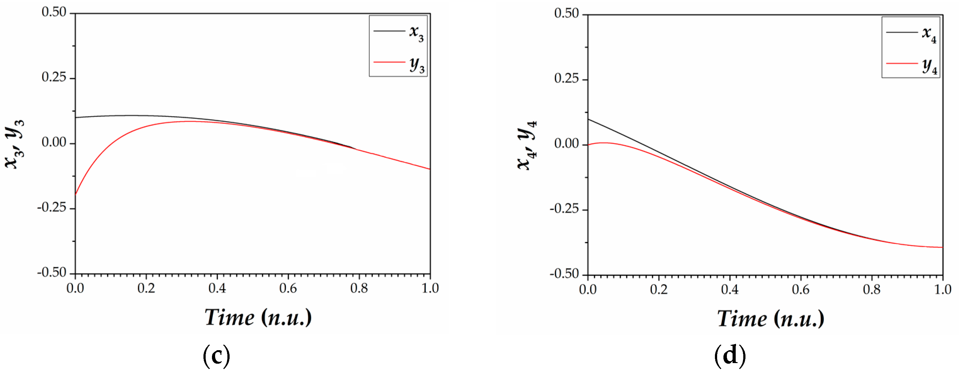
Furthermore, the set of initial conditions of the master system (8), is (x1(0), x2(0), x3(0), x4(0)) = (0.1, 0.1, 0.1, 0.1), while the set of initial conditions of the slave system (13), is (y1(0), y2(0), y3(0), x4(0)) = (–0.1, 0.2, –0.2, 0). In addition, we use the values of , as initial conditions of the parameter estimates. The synchronization of the states of the master system (8) and slave system (13) are depicted in Figure 8, while the time-history of the synchronization errors e1(t), e2(t), e3(t), e4(t) is depicted in Figure 9. In more details, Figure 8 shows the fast convergence of the respective signals of the two coupled systems by using the proposed synchronization scheme. Furthermore, Figure 9 confirms the feasibility of the synchronization method in the coupled system by confirming that the synchronization errors converge to zero, as it is expected. Therefore, a chaotic complete synchronization has been achieved.
6. Discussion
This paper focuses on the study of a 4D hyperchaotic hyperjerk dynamical system (8) with only two nonlinear terms. Recently, Elhadj and Sprott indicated that the hyperjerk form (3) can describe all periodically forced oscillators and many of the coupled oscillators [11]. Therefore, the proposed system (8) could be a suitable candidate for use in order to model such kind of oscillators. As proved, the maximal Lyapunov exponent (MLE) and the Kaplan–Yorke dimension of the proposed hyperchaotic system (8) is greater than the respective features of the other hyperjerk systems of the same category, which has been presented in literature. Therefore, the high-dimensional phase space of the hyperjerk system (8) combined with its high Kaplan–Yorke dimension, which guarantees the system’s complex dynamical behavior, contributes to the required robustness. In addition, the proposed system (8) is a dissipative system for c > 0 and it has an unstable equilibrium point at E(0, 0, 0, 0). Furthermore, it is invariant under the coordinate transformation (x1, x2, x3, x4) → (−x1, −x2, −x3, x4), which is a very important feature that could drive the system to coexisting attractors.
The dynamical behavior of system (8) has been studied using well-known tools of nonlinear theory, such as bifurcation diagrams, Lyapunov exponents, phase portraits and Poincaré maps. The effect of the parameter a is investigated and the route to chaos through a quasiperiodic behavior, in a narrow band, is driven to hyperchaos, which is maintained in a large range of values of the parameter a. The quasiperiodic behavior has been confirmed by the closed loop, which is produced in system’s Poincaré map, for a selected value of the parameter a (a = 4.209) from quasiperiodic’s narrow band region. Therefore, despite its simplicity, the system has an enlarged area of hyperchaotic behavior, which is not so usual in other systems of this family.
In order to explore the feasibility of the proposed hyperchaotic system (8), the classical approach, by using the physical realization through the design of an electronic circuit, has been adopted. For this reason, common off-the-shelf electronic components, such as op-amps and multipliers, have been used in this work. PSpice results confirm the good agreement between the circuit’s simulation results and numerical results. In more details, the circuit’s phase portraits that have been produced by using the PSpice are identical in form and size with the respective system’s simulated ones. Therefore, the proposed system could be used as a hyperchaotic generator in many practical applications, such as in encryption and secure communication schemes.
Furthermore, an adaptive synchronization scheme for a system of two coupled 4D hyperchaotic hyperjerk systems has been developed. For the obtained, with this method, the main adaptive results are proved by using Lyapunov stability theory. The effectiveness of the proposed synchronization scheme is proved from the simulation results, in which the fast convergence of the signals of the two coupled systems has been achieved.
One of the possible future research directions is the investigation of the coexistence of multiple attractors, based on system’s invariance. In addition, the experimental realization of the circuit that is designed and presented in this work will be done in the near future. Finally, an engineering application, such as an encryption or secure communication, based on the proposed 4D hyperchaotic hyperjerk dynamical system may be designed.
Acknowledgments
This research was partially funded by the Special Account for Research Grants of the National and Kapodistrian University of Athens
Author Contributions
Christos K. Volos and Hector E. Nistazakis studied the system’s dynamics; Petros A. Daltzis designed and simulated the circuit; Andreas D. Tsigopoulos and George S. Tombras designed the adaptive control law for globally and exponentially synchronizing the identical 4D hyperchaotic hyperjerk systems with unknown system’s parameters. Petros A. Daltzis wrote the paper.
Conflicts of Interest
The authors declare no conflict of interest.
References
- Rössler, O.E. An equation for hyperchaos. Phys. Lett. A 1979, 71, 155157. [Google Scholar] [CrossRef]
- Jia, Q. Hyperchaos generated from the Lorenz chaotic system and its control. Phys. Lett. A 2007, 366, 217–222. [Google Scholar] [CrossRef]
- Chen, A.; Lu, J.; Lü, J.; Yu, S. Generating hyperchaotic Lü attractor via state feedback control. Physics A 2006, 364, 103–110. [Google Scholar] [CrossRef]
- Li, X. Modified projective synchronization of a new hyperchaotic system via nonlinear control. Commun. Theor. Phys. 2009, 52, 274–278. [Google Scholar]
- Wang, J.; Chen, Z. A novel hyperchaotic system and its complex dynamics. Int. J. Bifurcat. Chaos 2008, 18, 3309–3324. [Google Scholar] [CrossRef]
- Ghost, D.; Bhattacharya, S. Projective synchronization of new hyperchaotic system with fully unknown parameters. Nonlinear Dyn. 2010, 61, 11–21. [Google Scholar]
- Jia, Q. Projective synchronization of a new hyperchaotic Lorenz system. Phys. Lett. A 2007, 370, 40–45. [Google Scholar] [CrossRef]
- Vaidyanathan, S. A ten-term novel 4-D hyperchaotic system with three quadratic nonlinearities and its control. Int. J. Control Theory Appl. 2013, 6, 97–109. [Google Scholar]
- Schot, S.H. Jerk: The time rate of change of acceleration. Am. J. Phys. 1978, 46, 1090–1094. [Google Scholar] [CrossRef]
- Coullet, P.; Tresser, C.; Arneodo, A. A transition to stochasticity for a class of forced oscillators. Phys. Lett. A 1979, 72, 268–270. [Google Scholar] [CrossRef]
- Elhadj, Z.; Sprott, J.C. Transformation of 4-D dynamical systems to hyperjerk form. Palestine J. Math. 2013, 2, 38–45. [Google Scholar]
- Ott, E.; Grebogi, C.; Yorke, J.A. Controlling chaos. Phys. Rev. Lett. 1990, 64, 1196–1199. [Google Scholar] [CrossRef] [PubMed]
- Huang, L.; Feng, R.; Wang, M. Synchronization of chaotic systems via nonlinear control. Phys. Lett. A 2004, 320, 271–275. [Google Scholar] [CrossRef]
- Vaidyanathan, S.; Azar, A.T.; Rajagopal, K.; Alexander, P. Design and SPICE implementation of a 12-term novel hyperchaotic system and its synchronization via active control. Int. J. Model. Identif. Control 2015, 23, 267–277. [Google Scholar] [CrossRef]
- Baz, A.; Poh, S. Performance of an active control system with piezoelectric actuators. J. Sound Vib. 1988, 126, 327–343. [Google Scholar] [CrossRef]
- Åström, K.J.; Wittenmark, B. Adaptive Control; Courier Corporation: North Chelmsford, MA, USA, 2013. [Google Scholar]
- Craig, J.J.; Hsu, P.; Sastry, S.S. Adaptive control of mechanical manipulators. Int. J. Robot. Res. 1987, 6, 16–28. [Google Scholar] [CrossRef]
- Vaidyanathan, S.; Volos, C.K.; Pham, V.T. Hyperchaos, adaptive control and synchronization of a novel 5-Dhyperchaotic system with three positive Lyapunov exponents and its SPICE implementation. Arch. Control Sci. 2014, 24, 409–446. [Google Scholar]
- Yang, T.; Chua, L.O. Control of chaos using sampled-data feedback control. Int. J. Bifurcat. Chaos 1999, 9, 215–219. [Google Scholar] [CrossRef]
- Li, N.; Zhang, Y.; Hu, J.; Nie, Z. Synchronization for general complex dynamical networks with sampled-data. Neurocomputing 2011, 74, 805–811. [Google Scholar] [CrossRef]
- Park, J.H.; Kwon, O.M. A novel criterion for delayed feedback control of time-delay chaotic systems. Chaos Soliton Fract. 2003, 17, 709–716. [Google Scholar] [CrossRef]
- Sun, J. Delay-dependent stability criteria for time-delay chaotic systems via time-delay feedback control. Chaos Soliton Fract. 2004, 21, 143–150. [Google Scholar] [CrossRef]
- Vaidyanathan, S.; Idowu, B.A.; Azar, A.T. Backstepping controller design for the global chaos synchronization of Sprott’s jerk systems. In Chaos Modeling and Control Systems Design; Azar, A.T., Vaidyanathan, S., Eds.; Springer: Basel, Switzerland, 2015; Volume 581, pp. 39–58. [Google Scholar]
- Yang, J.H.; Wu, J.; Hu, Y.M. Backstepping method and its applications to nonlinear robust control. Control Decis. 2002, 17, 641–647. [Google Scholar]
- Chen, X.; Park, J.H.; Cao, J.; Qiu, J. Sliding mode synchronization of multiple chaotic systems with uncertainties and disturbances. Appl. Math. Comput. 2017, 308, 161–173. [Google Scholar] [CrossRef]
- Chen, X.; Park, J.H.; Cao, J.; Qiu, J. Adaptive synchronization of multiple uncertain coupled chaotic systems via sliding mode control. Neurocomputing 2018, 273, 9–21. [Google Scholar] [CrossRef]
- Huang, X.; Cao, J.; & Li, Y. Takagi-Sugeno fuzzy-model-based control of hyperchaotic Chen system with norm-bounded uncertainties. Proc. Inst. Mech. Eng. Part I J. Syst. Control Eng. 2010, 224, 223–234. [Google Scholar] [CrossRef]
- Lu, J.; Cao, J. Adaptive complete synchronization of two identical or different chaotic (hyperchaotic) systems with fully unknown parameters. Chaos 2005, 15, 043901. [Google Scholar] [CrossRef] [PubMed]
- Liao, T.L. Adaptive synchronization of two Lorenz systems. Chaos Soliton Fract. 1998, 9, 1555–1561. [Google Scholar] [CrossRef]
- Feki, M. An adaptive chaos synchronization scheme applied to secure communication. Chaos Soliton Fract. 2003, 18, 141–148. [Google Scholar] [CrossRef]
- Kocarev, L.; Parlitz, U. General approach for chaos synchronization with applications to communications. Phys. Rev. Lett. 1995, 74, 5028–5030. [Google Scholar] [CrossRef] [PubMed]
- Murali, K.; Lakshmanan, M. Secure communication using a compound signal using sampled-data feedback. J. Appl. Math. Mech. 2003, 11, 1309–1315. [Google Scholar]
- Yang, J.; Zhu, F. Synchronization for chaotic systems and chaos-based secure communications via both reduced-order and step-by-step sliding mode observers. Commun. Nonlinear Sci. Numer. Simul. 2013, 18, 926–937. [Google Scholar] [CrossRef]
- Daltzis, P.A.; Volos, C.K.; Nistazakis, H.E.; Tzanakaki, A.Α.; Tombras, G.S. Synchronization of Hyperchaotic Hyperjerk circuits with application in secure communications. In Proceedings of the 7th International Conference on “Experiments/Process/System Modeling/Simulation/Optimization—IC-EPSMSO”, Athens, Greece, 5–8 July 2017. [Google Scholar]
- Kocarev, L. Chaos-based cryptography: A brief overview. IEEE Trans. Circuits Syst. I 2001, 1, 6–21. [Google Scholar] [CrossRef]
- Volos, C.K.; Kyprianidis, I.M.; Stouboulos, I.N. Experimental demonstration of a chaotic cryptographic scheme. WSEAS Trans. Circuits Syst. 2006, 5, 1654–1661. [Google Scholar]
- Wang, Y.; Wang, K.W.; Liao, X.; Chen, G. A new chaos-based fast image encryption. Appl. Soft Comput. 2011, 11, 514–522. [Google Scholar] [CrossRef]
- Zhang, X.; Zhao, Z.; Wang, J. Chaotic image encryption based on circular substitution box and key stream buffer. Signal Process. Image Commun. 2014, 29, 902–913. [Google Scholar] [CrossRef]
- Fujisaka, H.; Yamada, T. Stability theory of synchronized motion in coupled-oscillator systems. Prog. Theor. Phys. 1983, 69, 32–47. [Google Scholar] [CrossRef]
- Pecora, L.M.; Carroll, T.L. Synchronization in chaotic systems. Phys. Rev. Lett. 1990, 64, 821–824. [Google Scholar] [CrossRef] [PubMed]
- Pecora, L.M.; Carroll, T.L. Synchronizing chaotic circuits. IEEE Trans. Circuits Syst. 1991, 38, 453–456. [Google Scholar]
- Liu, Y.; Takiguchi, Y.; Davis, P.; Aida, T.; Saito, S.; Liu, J.M. Experimental observation of complete chaos synchronization in semiconductor lasers. Appl. Phys. Lett. 2002, 80, 4306–4308. [Google Scholar] [CrossRef]
- Mahmoud, G.M.; Mahmoud, E.E. Complete synchronization of chaotic complex nonlinear systems with uncertain parameters. Nonlinear Dyn. 2010, 62, 875–882. [Google Scholar] [CrossRef]
- Rosenblum, M.G.; Pikovsky, A.S.; Kurths, J. Phase synchronization of chaotic oscillators. Phys. Rev. Lett. 1996, 76, 1804. [Google Scholar] [CrossRef] [PubMed]
- Ge, Z.M.; Chen, C.C. Phase synchronization of coupled chaotic multiple time scales systems. Chaos Soliton Fract. 2004, 20, 639–647. [Google Scholar] [CrossRef]
- Wang, Y.W.; Guan, Z.H. Generalized synchronization of continuous chaotic system. Chaos Soliton Fract. 2006, 27, 97–101. [Google Scholar] [CrossRef]
- Rulkov, N.F.; Sushchik, M.M.; Tsimring, L.S.; Abarbanel, H.D. Generalized synchronization of chaos in directionally coupled chaotic systems. Phys. Rev. E 1995, 51, 980. [Google Scholar] [CrossRef]
- Vaidyanathan, S.; Sampath, S. Anti-synchronization of identical chaotic systems via novel sliding control method with application to Vaidyanathan—Madhavan chaotic system. Int. J. Control Theory Appl. 2016, 9, 85–100. [Google Scholar]
- Kim, C.M.; Rim, S.; Kye, W.H.; Ryu, J.W.; Park, Y.J. Anti-synchronization of chaotic oscillators. Phys. Lett. A 2003, 320, 39–46. [Google Scholar] [CrossRef]
- Vaidyanathan, S. Generalized projective synchronization of novel 3-D chaotic systems with an exponential non-linearity via active and adaptive control. Int. J. Control Theory Appl. 2014, 22, 207–217. [Google Scholar]
- Sivaperumal, S. Hybrid synchronization of identical chaotic systems via novel sliding control with application to hyperchaotic Vaidyanathan—Volos system. Int. J. Control Theory Appl. 2016, 9, 261–278. [Google Scholar]
- Park, J.H. Adaptive synchronization of hyperchaotic Chen system with uncertain parameters. Chaos Soliton Fract. 2005, 26, 959–964. [Google Scholar] [CrossRef]
- Chlouverakis, K.E.; Sprott, J.C. Chaotic hyperjerk systems. Chaos Soliton Fract. 2006, 28, 739–746. [Google Scholar] [CrossRef]
- Grassberger, P.; Procaccia, I. Measuring the strangeness of strange attractors. Physica D 1983, 9, 189–208. [Google Scholar] [CrossRef]
- Grassberger, P.; Procaccia, I. Characterization of strange attractors. Phys. Rev. Lett. 1983, 50, 346–349. [Google Scholar] [CrossRef]
- Strogatz, S.H. Nonlinear Dynamics and Chaos: With Applications to Physics, Biology, Chemistry, and Engineering; Perseus Books: Cambridge, MA, USA, 1994. [Google Scholar]
- Daltzis, P.; Vaidyanathan, S.; Pham, V.T.; Volos, C.; Nistazakis, E.; Tombras, G. Hyperchaotic attractor in a novel hyperjerk system with two nonlinearities. Circ. Syst. Signal Proc. 2017, 2017, 1–23. [Google Scholar] [CrossRef]
- Wolf, A.; Swift, J.B.; Swinney, H.L.; Vastano, J.A. Determining Lyapunov exponents from a time series. Physica D 1985, 16, 285–317. [Google Scholar] [CrossRef]
- Vaidyanathan, S.; Volos, C.K.; Pham, V.T.; Madhavan, K. Analysis, adaptive control and synchronization of a novel 4-D hyperchaotic hyperjerk system and its SPICE implementation. Arch. Control Sci. 2015, 25, 135–158. [Google Scholar] [CrossRef]
- Vaidyanathan, S. Analysis, adaptive control and synchronization of a novel 4-D hyperchaotic hyperjerk system via backstepping control method. Arch. Control Sci. 2016, 26, 311–338. [Google Scholar] [CrossRef]
- Pham, V.T.; Vaidyanathan, S.; Volos, C.K.; Jafari, S.; Wang, X. A chaotic hyperjerk system based on memristive device. In Advances and Applications in Chaotic Systems; Springer: Berlin, Germany, 2016; pp. 39–58. [Google Scholar]
- Wang, X.; Vaidyanathan, S.; Volos, C.K.; Pham, V.T.; Kapitaniak, T. Dynamics, circuit realization, control and synchronization of a hyperchaotic hyperjerk system with coexisting attractors. Nonlinear Dyn. 2017, 89, 1673–1687. [Google Scholar] [CrossRef]
- Vaidyanathan, S. A conservative hyperchaotic hyperjerk system based on memristive device. In Advances in Memristors, Memristive Devices and Systems; Springer: Berlin, Germany, 2017; pp. 393–423. [Google Scholar]
- Yalcin, M.E.; Suykens, J.A.K.; Vandewalle, J. True random bit generation from a double-scroll attractor. IEEE Trans. Circuits Syst. I Regul. Pap. 2004, 51, 1395–1404. [Google Scholar] [CrossRef]
- Ergun, S.; Ozoguz, S. Truly random number generators based on a nonautonomous chaotic oscillator. AEÜ Int. J. Electron. Commun. 2007, 61, 235–242. [Google Scholar] [CrossRef]
- Cavusoglu, U.; Akgul, A.; Kacar, S.; Pehlivan, I.; Zengin, A. A novel chaos-based encryption algorithm over TCP data packet for secure communication. Secur. Commun. Netw. 2016, 9, 1285–1296. [Google Scholar] [CrossRef]
- Kacar, S. Analog circuit and microcontroller based RNG application of a new easy realizable 4D chaotic system. Optik 2016, 127, 9551–9561. [Google Scholar] [CrossRef]
- Lin, Z.; Yu, S.; Li, C.; Lü, J.; Wang, Q. Design and smartphone-based implementation of a chaotic video communication scheme via wan remote transmission. Int. J. Bifurcat. Chaos 2016, 26, 1650158. [Google Scholar] [CrossRef]
- Liu, H.; Kadir, A.; Li, Y. Audio encryption scheme by confusion and diffusion based on multi-scroll chaotic system and one-time keys. Optik 2016, 127, 7431–7438. [Google Scholar] [CrossRef]
- Volos, C.K.; Kyprianidis, I.M.; Stouboulos, I.N. A chaotic path planning generator for autonomous mobile robots. Robot. Auton. Syst. 2012, 60, 651–656. [Google Scholar] [CrossRef]
- Varnosfaderani, I.S.; Sabahi, M.F.; Ataei, M. Joint blind equalization and detection in chaotic communication systems using simulation-based methods. AEÜ Int. J. Electron. Commun. 2015, 69, 1445–1452. [Google Scholar] [CrossRef]
- Abdullah, A.H.; Enayatifar, R.; Lee, M. A hybrid genetic algorithm and chaotic function model for image encryption. AEÜ Int. J. Electron. Commun. 2012, 66, 806–816. [Google Scholar] [CrossRef]
- Zhang, Q.; Liu, L.; Wei, X. Improved algorithm for image encryption based on DNA encoding and multi-chaotic maps. AEÜ Int. J. Electron. Commun. 2014, 69, 186–1892. [Google Scholar] [CrossRef]
- Zhang, Y.; Xiao, D. Self-adaptive permutation and combined global diffusion for chaotic color image encyption. AEÜ Int. J. Electron. Commun. 2014, 68, 361–368. [Google Scholar] [CrossRef]
- Min, L.; Yang, X.; Chen, G.; Wang, D. Some polynomial chaotic maps without equilibria and an application to image encryption with avalanche effects. Int. J. Bifurcat. Chaos 2015, 25, 1550124. [Google Scholar] [CrossRef]
- Elwakil, A.S.; Ozoguz, S. Chaos in a pulse-excited resonator with self feedback. Electron. Lett. 2003, 39, 831–833. [Google Scholar] [CrossRef]
- Piper, J.R.; Sprott, J.C. Simple autonomous chaotic circuits. IEEE Trans. Circuits Syst. II Exp. Briefs 2010, 57, 730–734. [Google Scholar] [CrossRef]
- Trejo-Guerra, R.; Tlelo-Cuautle, E.; Jimenez-Fuentes, J.M.; Sanchez-Lopez, C.; Munoz-Pacheco, J.M.; Espinosa-Flores-Verdad, G.; Rocha-Perez, J.M. Integrated circuit generating 3- and 5-scroll attractors. Commun. Nonlinear Sci. Numer. Simul. 2012, 17, 4328–4335. [Google Scholar] [CrossRef]
- Trejo-Guerra, R.; Tlelo-Cuautle, E.; Jimenez-Fuentes, J.M.; Munoz-Pacheco, J.M.; Sanchez-Lopez, C. Multi-scroll floating gate-based integrated chaotic oscillator. Int. J. Circuit Theory Appl. 2013, 41, 831–843. [Google Scholar] [CrossRef]
- Pano-Azucena, A.D.; Rangel-Magdaleno, J.J.; Tlelo-Cuautle, E.; Quintas-Valles, A.J. Arduino-based chaotic secure communication system using multi-directional multi-scroll chaotic oscillators. Nonlinear Dyn. 2017, 87, 2203–2217. [Google Scholar] [CrossRef]
- Koyuncu, I.; Ozcerit, A.T.; Pehlivan, I. Implementation of FPGA-based real time novel chaotic oscillator. Nonlinear Dyn. 2014, 77, 49–59. [Google Scholar] [CrossRef]
- Tlelo-Cuautle, E.; Rangel-Magdaleno, J.J.; Pano-Azucena, A.D.; Obeso-Rodelo, P.J.; Nunez-Perez, J.C. FPGA realization of multi-scroll chaotic oscillators. Commun. Nonlinear Sci. Numer. Simul. 2015, 27, 66–80. [Google Scholar] [CrossRef]
- Tlelo-Cuautle, E.; Pano-Azucena, A.D.; Rangel-Magdaleno, J.J.; Carbajal-Gomez, V.H.; Rodriguez-Gomez, G. Generating a 50-scroll chaotic attractor at 66 MHz by using FPGAs. Nonlinear Dyn. 2016, 85, 2143–2157. [Google Scholar] [CrossRef]
- Khalil, H.K. Nonlinear Systems, 3rd ed.; Prentice Hall: Upper Saddle River, NJ, USA, 2001. [Google Scholar]
Figure 1.
Hyperchaotic attractors of system (8) in (a) x1–x2 plane; (b) x1–x3 plane; (c) x1–x4; (d) x2–x3 plane; (e) x2–x4 plane and (f) x3–x4 plane, for a = 3.8, b = 0.1 and c = 1.5 and initial conditions (x1(0), x2(0), x3(0), x4(0)) = (0.1, 0.1, 0.1, 0.1).
Figure 1.
Hyperchaotic attractors of system (8) in (a) x1–x2 plane; (b) x1–x3 plane; (c) x1–x4; (d) x2–x3 plane; (e) x2–x4 plane and (f) x3–x4 plane, for a = 3.8, b = 0.1 and c = 1.5 and initial conditions (x1(0), x2(0), x3(0), x4(0)) = (0.1, 0.1, 0.1, 0.1).

Figure 2.
Poincaré maps of system (8) in (a) x1–x3 plane and (b) x1–x4 plane, for a = 3.8, b = 0.1 and c = 1.5 and initial conditions (x1(0), x2(0), x3(0), x4(0)) = (0.1, 0.1, 0.1, 0.1).
Figure 2.
Poincaré maps of system (8) in (a) x1–x3 plane and (b) x1–x4 plane, for a = 3.8, b = 0.1 and c = 1.5 and initial conditions (x1(0), x2(0), x3(0), x4(0)) = (0.1, 0.1, 0.1, 0.1).

Figure 3.
Bifurcation diagram of system (8)’s variable x4 versus the parameter a, for b = 0.1 and c = 1.5.
Figure 3.
Bifurcation diagram of system (8)’s variable x4 versus the parameter a, for b = 0.1 and c = 1.5.
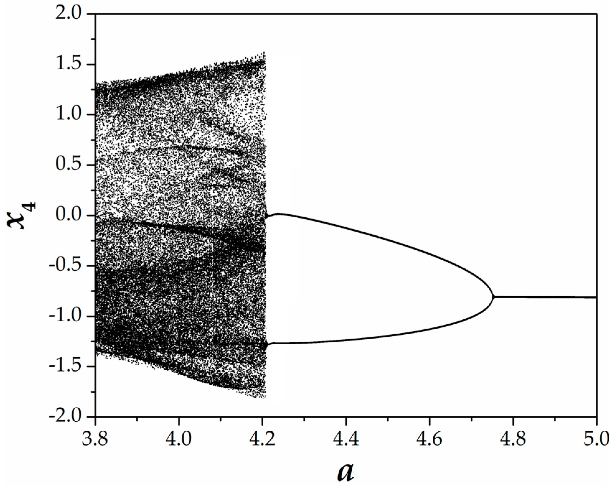
Figure 4.
Spectrum of three largest Lyapunov exponents of system (8) versus the parameter a, for b = 0.1 and c = 1.5.
Figure 4.
Spectrum of three largest Lyapunov exponents of system (8) versus the parameter a, for b = 0.1 and c = 1.5.

Figure 5.
Phase portraits in x1–x2 plane and the respective Poincaré maps in x1–x3 plane, for (a,b) a = 5 (period-1 state); (c,d) a = 4.5 (period-2 state); and (e,f) a = 4.209 (quasiperiodic state). The rest of the parameters and initial conditions are: b = 0.1 and c = 1.5 and (x1(0), x2(0), x3(0), x4(0)) = (0.1, 0.1, 0.1, 0.1).


Figure 6.
Schematic of the designed circuit for the proposed system (8).

Figure 7.
PSpice simulation results of system (8) in different phase portraits (a) x1–x2 plane; (b) x1–x3 plane; (c) x1–x4; (d) x2–x3 plane; (e) x2–x4 plane and (f) x3–x4 plane, for a = 3.8, b = 0.1 and c = 1.5 and initial conditions (x1(0), x2(0), x3(0), x4(0)) = (0.1, 0.1, 0.1, 0.1).
Figure 7.
PSpice simulation results of system (8) in different phase portraits (a) x1–x2 plane; (b) x1–x3 plane; (c) x1–x4; (d) x2–x3 plane; (e) x2–x4 plane and (f) x3–x4 plane, for a = 3.8, b = 0.1 and c = 1.5 and initial conditions (x1(0), x2(0), x3(0), x4(0)) = (0.1, 0.1, 0.1, 0.1).
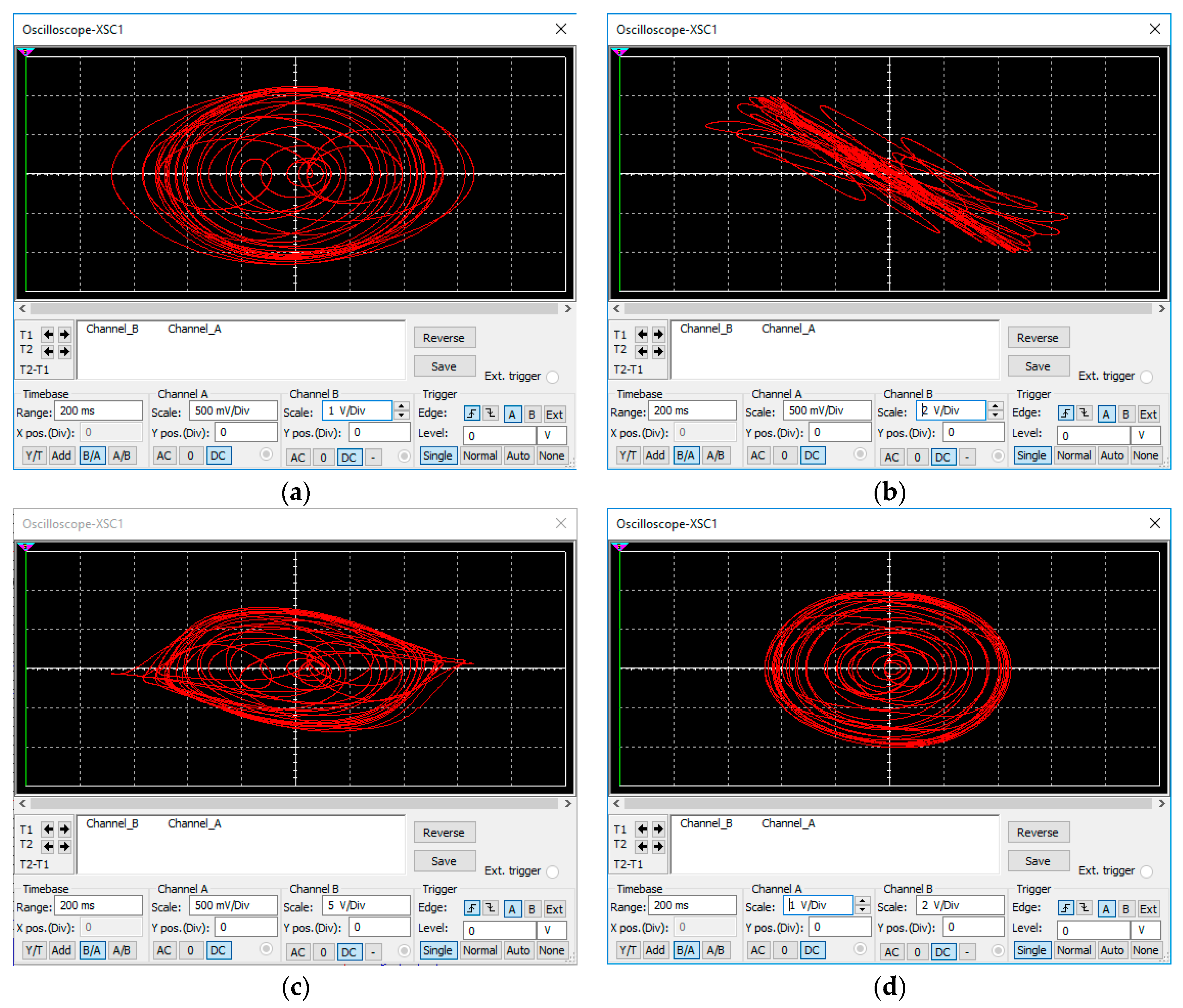
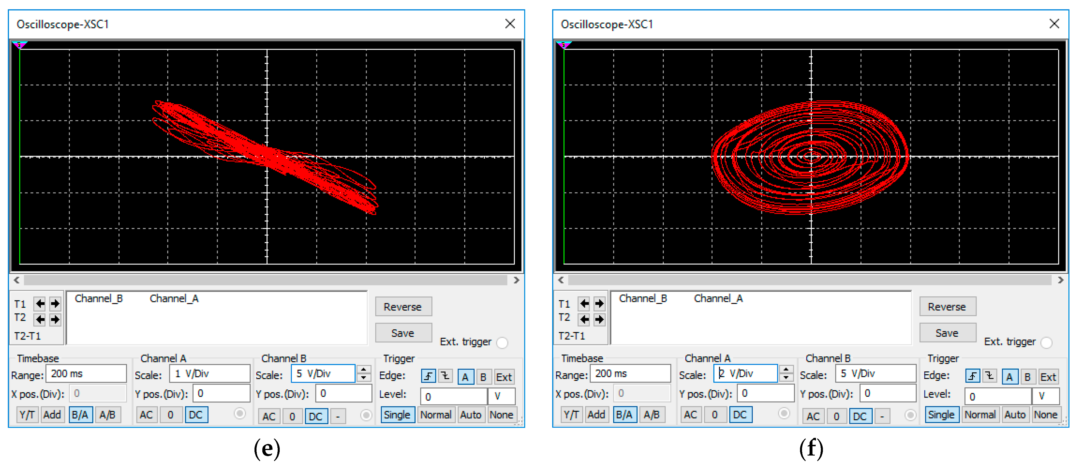
Figure 8.
Synchronization of the states (a) x1(t) and y1(t); (b) x2(t) and y2(t); (c) x3(t) and y3(t) and (d) x4(t) and y4(t).
Figure 8.
Synchronization of the states (a) x1(t) and y1(t); (b) x2(t) and y2(t); (c) x3(t) and y3(t) and (d) x4(t) and y4(t).
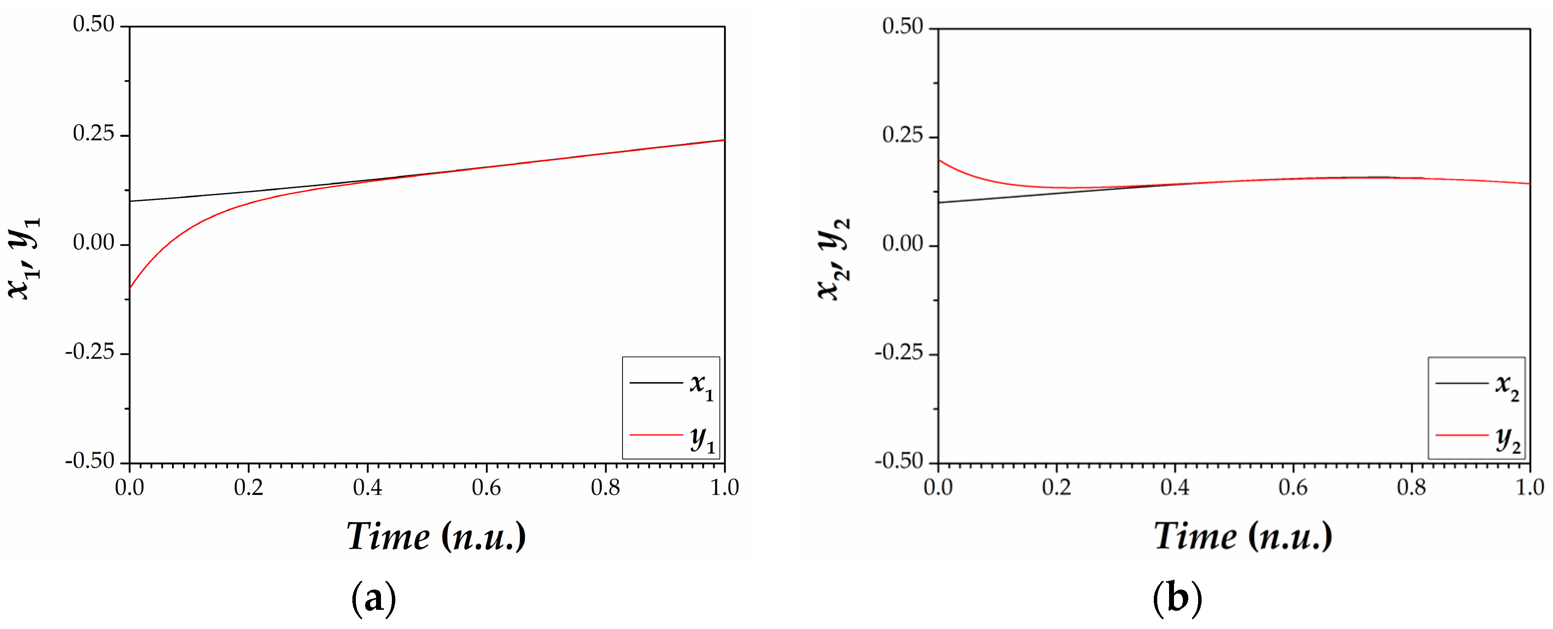

Figure 9.
Time-series of the synchronization errors ei(t), (i = 1, 2, 3, 4).

Table 1.
Comparison of system (8) with other reported hyperchaotic hyperjerk systems regarding the maximal Lyapunov exponent and the Kaplan–Yorke dimension.
Table 1.
Comparison of system (8) with other reported hyperchaotic hyperjerk systems regarding the maximal Lyapunov exponent and the Kaplan–Yorke dimension.
| Reported Work | Maximal Lypunov Exponent | Kaplan–Yorke Dimension |
|---|---|---|
| [53] | 0.1320 | 3.1300 |
| [57] | 0.1555 | 3.1171 |
| [59] | 0.1448 | 3.1573 |
| [60] | 0.1422 | 3.1348 |
| [61] | 0.0730 | 3.1300 |
| [62] | 0.1250 | 3.1325 |
| [63] | 0.1320 | 3.1300 |
| This work | 0.1809 | 3.1405 |
© 2018 by the authors. Licensee MDPI, Basel, Switzerland. This article is an open access article distributed under the terms and conditions of the Creative Commons Attribution (CC BY) license (http://creativecommons.org/licenses/by/4.0/).
Share and Cite
MDPI and ACS Style
Daltzis, P.A.; Volos, C.K.; Nistazakis, H.E.; Tsigopoulos, A.D.; Tombras, G.S. Analysis, Synchronization and Circuit Design of a 4D Hyperchaotic Hyperjerk System. Computation 2018, 6, 14. https://doi.org/10.3390/computation6010014
AMA Style
Daltzis PA, Volos CK, Nistazakis HE, Tsigopoulos AD, Tombras GS. Analysis, Synchronization and Circuit Design of a 4D Hyperchaotic Hyperjerk System. Computation. 2018; 6(1):14. https://doi.org/10.3390/computation6010014
Chicago/Turabian StyleDaltzis, Petros A., Christos K. Volos, Hector E. Nistazakis, Andreas D. Tsigopoulos, and George S. Tombras. 2018. "Analysis, Synchronization and Circuit Design of a 4D Hyperchaotic Hyperjerk System" Computation 6, no. 1: 14. https://doi.org/10.3390/computation6010014
Note that from the first issue of 2016, this journal uses article numbers instead of page numbers. See further details here.