Application of High-Order Compact Difference Scheme in the Computation of Incompressible Wall-Bounded Turbulent Flows


1
Research Center for Applied Mechanics, School of Mechano-Electronic Engineering, Xidian University, Xi’an 710071, China
2
Key Laboratory of Mechanics on Disaster and Environment in Western China (Lanzhou University), Ministry of Education, Lanzhou 730000, China
*
Author to whom correspondence should be addressed.
Computation 2018, 6(2), 31; https://doi.org/10.3390/computation6020031
Submission received: 6 March 2018
/
Revised: 29 March 2018
/
Accepted: 4 April 2018
/
Published: 11 April 2018
(This article belongs to the Section Computational Engineering)
Abstract
:In the present work, a highly efficient incompressible flow solver with a semi-implicit time advancement on a fully staggered grid using a high-order compact difference scheme is developed firstly in the framework of approximate factorization. The fourth-order compact difference scheme is adopted for approximations of derivatives and interpolations in the incompressible Navier–Stokes equations. The pressure Poisson equation is efficiently solved by the fast Fourier transform (FFT). The framework of approximate factorization significantly simplifies the implementation of the semi-implicit time advancing with a high-order compact scheme. Benchmark tests demonstrate the high accuracy of the proposed numerical method. Secondly, by applying the proposed numerical method, we compute turbulent channel flows at low and moderate Reynolds numbers by direct numerical simulation (DNS) and large eddy simulation (LES). It is found that the predictions of turbulence statistics and especially energy spectra can be obviously improved by adopting the high-order scheme rather than the traditional second-order central difference scheme.
1. Introduction
The study of wall-bounded turbulent flows advanced a lot and benefited from high-fidelity numerical simulations [1,2,3], i.e., direct numerical simulation (DNS) and large eddy simulation (LES). The spectral method is the most popular for the simulation of wall-bounded turbulent flows like channel flow [4,5,6,7,8,9] and pipe flow [10,11,12,13] because of its inherently high accuracy. However, it is limited to simple rather than complex geometries, and the latter are more common in industrial and environmental flows. For instance, it is very difficult to apply the spectral/pseudospectral method in the computation of atmospheric flow over complex terrains. In comparison, the finite difference (FD) and finite volume (FV) methods are much more flexible and have been widely used in practical applications, while mostly with second-order accuracy only. Therefore, it is always a demanding task to design a numerical method to have both high-order accuracy and enough flexibility in complex geometry. It is noted that the second-order accurate central difference scheme on a staggered grid [14] has yielded much success in turbulence simulation due to the exact conservation of discrete kinetic energy in the absence of viscosity [15,16]. However, it is always believed that the truncation error of a low-order finite difference scheme may be as large as the subgrid-scale terms in LES [17]. Therefore, a high-order scheme is preferred. High-order energy-conserving FD/FV methods have been proposed by [18,19], among others, with many successful applications. While the present interest is another type of scheme, i.e., the compact difference scheme [20], its advantage is the very compact stencil points to achieve high order, and we aim to study whether it can provide help in wall turbulence simulation.
The popularity of the compact difference scheme in various branches of the computational fluid dynamics (CFD) should be ascribed to [20]. In this seminal work, the classical Páde approximation was generalized for the evaluations of derivative, interpolation and filtering. Improved spectral-like behaviors have been demonstrated in a variety of applications. Since then, a lot of extensions and applications of the compact difference scheme have been reported. The original work of [20] and many later developments [21,22,23,24,25,26] were mainly for the compressible flow, while the present study focuses only on the incompressible flow. The velocity–pressure coupling is one of the main challenges for numerical simulation of incompressible flow, and many different approaches have been successfully proposed and applied, e.g., the SIMPLE (Semi-Implicit Method for Pressure-Linked Equations)-class method [27,28,29], the artificial-compressibility formulation [30,31,32], and the fractional-step or the projection method [33,34,35,36,37,38], among many others. For the general knowledge of incompressible flow computation, some comprehensive monographs are recommended [27,39,40].
In an early study, Ma et al. [41] discretized the convection terms of the incompressible Navier–Stokes equation by a fifth-order-accurate upwind compact difference scheme, the viscous terms by a sixth-order symmetrical compact difference scheme, and the continuity equation and the pressure gradient terms were approximated by a standard fourth-order finite difference scheme. Demuren et al. [42] applied fourth- and sixth-order compact difference schemes for spatial discretization on a collocated grid, and found the odd–even decoupling problem was surprisingly eliminated. The applications of their method were given in [43]. In recent years, there has been increasing interest in utilizing the compact difference scheme for spatial discretization of the incompressible Navier–Stokes equations combined with the projection method for velocity–pressure decoupling [44,45,46,47,48,49,50,51,52,53]. Differences among these works can be classified into three aspects: (a) the first is the grid arrangement. It is well known that the staggered grid can perfectly prevent the odd-even decoupling problem in the computation of an incompressible flow. Although Demuren et al. [42] reported successful applications of the compact difference scheme on a collocated grid, the staggered grid is still the best option. Another grid arrangement style beyond the classical fully staggered grid is the so-called half-staggered grid, on which the velocity components are all located at cell corners and the pressure is defined at the cell center [48,50]. The spurious pressure oscillations were also successfully suppressed; (b) the second is the temporal discretization. Since the derivatives and the unknowns are related to its neighboring ones, the compact difference scheme is actually an implicit formulation and it is nontrivial to implement an implicit time-advancing scheme additionally. Therefore, most of the above studies incorporated explicit time-advancing methods like Runge–Kutta or Adams–Bashforth schemes. Knikker [47] treated the viscous diffusion terms by a semi-implicit Crank–Nicolson scheme, while an iterative algorithm was used to solve the linear system. In a recent study, Abide et al. [53] realized a semi-implicit time advancement with a compact scheme using a parallelized matrix diagonalization approach; and (c) the last issue is about the pressure Poisson equation. With the usage of a high-order compact scheme for the continuity equation and the pressure gradient term, the coefficient matrix of the linear system of the discrete pressure Poisson equation is not sparse, so that many efficient numerical methods for sparse linear systems can not be applied anymore. Boersma [49] and Tyliszczak [50] both solved the Poisson equation iteratively using the GMRESR algorithm. Reis et al. [51] reformulated the Poisson equation into a set of first-order differential equations, thus more efficient direct or iterative solvers for the sparse system could be used, but the computational cost was increased. On a half-staggered grid, Laizet and Lamballais [48] transformed and solved the Poisson equation in spectral space by the fast Fourier transform (FFT), and then obtained the solution in physical space by the inverse Fourier transform efficiently.
There are two main purposes of the present study. Firstly, we aim to develop a highly efficient solver for the incompressible flow with a high-order compact difference scheme and semi-implicit time advancement on a fully staggered grid. We choose the classical fully staggered grid other than the half-staggered grid [48,50] because the former one is much more widely used in research and applications. For the temporal discretization, larger time steps can be allowed if a semi-implicit Crank–Nicolson scheme is implemented for the viscous terms, and we propose a new method in the framework of approximate factorization [54,55,56] to significantly simplify the implementation. Therefore, the present method could be regarded as a further development of the approximate factorization method to a higher order. This is the major contribution of the present work to the numerical method, since it is not straightforward to couple a semi-implicit time advancement with an implicit compact difference scheme in spatial. Following [48], the FFT is adopted to solve the discrete Poisson equation as a highly efficient direct solver. The second purpose is to apply and test the present high-order numerical method on the computation of wall-bounded turbulent flows. We hope the adoption of the compact difference scheme could lead to more accurate results. There are few studies comparing different numerical methods for the DNS and/or LES of wall-bounded turbulence, at least to the authors’ knowledge.
The paper is arranged as follows. The numerical method is described in Section 2 and several validation tests are illustrated in Section 3. Section 4 details the application of the present numerical method in the computation of turbulent plane channel flows at low and high Reynolds numbers. The final conclusions are drawn in Section 5.
2. Numerical Method
2.1. Governing Equations
The governing equations are the non-dimensional incompressible Navier–Stokes equations, i.e.,
and the continuity equation
in which is the ith Cartesian coordinate, is the fluid velocity component in the ith direction, p is the pressure divided by fluid density implicitly, and is Reynolds number. All of the flow variables are non-dimensionalized by reference length and velocity. The initial condition is prescribed by a given velocity field. The boundary conditions for the velocity field can be Dirichlet or periodic.
2.2. Temporal Discretization
The Navier–Stokes Equation (1) are discretized temporally at the time level as [54,55,56]
where H is the discrete operator of the convection term in the divergence form, L is the discrete Laplacian operator, and G is the discrete gradient operator. From the discrete Equation (3), it is seen that the convection and viscous terms are discretized by the explicit Adams–Bashforth scheme and semi-implicit Crank–Nicolson scheme respectively, both of which are second-order accurate in time. In addition, is the time step and is the momentum boundary condition in the ith direction.
The temporally discretized continuity equation is written as
where D is the discrete divergence operator and is the boundary condition for mass conservation.
Following [55] among others [54,56], the temporally discretized Equations (3) and (4) are expressed in a matrix form, i.e.,
Here,
in which I is the unit matrix.
Equation (5) can be approximated by the block-LU decomposition [54,55,56] as
which is a second-order approximation of the original discretized Equation (5) temporally, i.e., the truncation error is [56], and can be separated into the following two equations:
in which is an intermediate velocity field. This approximate factorization can be regarded as a matrix form of the exact projection method.
Therefore, the whole projection procedure can be rewritten in a series of steps:
In the classical projection method [33,34,37,38], Equations (12) and (13) are the prediction step, and the pressure Poisson equation is solved in the step (14)–(16) are the correction step.
Following [56], Equation (12) can be further approximated preserving second-order temporal accuracy as
where , and are the discrete Laplacian operators in each Cartesian coordinate and L = + + . Thus, a highly efficient algorithm for the linear system (17) can be adopted, since the inversion of a large sparse matrix has been replaced by the inversions of three tridiagonal matrices [56]. This is also one key step for implementing a semi-implicit time advancement with a high-order compact scheme in the approximate factorization framework, which will be shown later.
The overall computation procedure is as follows:
2.3. Spatial Discretization
The discrete operators, i.e., L, D, G and H, are spatially discretized by the fourth-order compact difference scheme on a uniform grid, i.e., the Páde approximation [20].
We first look at the spatial discretization of first-order derivatives, i.e., the gradient operator G, the divergence operator D and the convection operator H, in the right-hand side of Equations (14) and (17). Taking the x direction, for example, the first-order derivative of a variable f on a staggered grid is approximated by
For the Dirichlet-type boundary condition, the one-sided fourth-order compact scheme proposed by [51] is used, which is
Since a fully staggered grid is adopted in the present formulation, the fourth-order compact interpolation scheme should also be incorporated in the evaluation of the convection operator H, which is
The spatial interpolations in other directions are similar.
The second-order derivative of f, e.g., the x-direction Laplacian operator , is discretized as
and the discretization of and is similar. Under the Dirichlet boundary condition, if we take u as f and consider the discretization of its second-order derivatives, the one-sided fourth-order scheme of [51] for the uniform collocated stencil is adopted as
In the other directions, we use the one-sided fourth-order scheme of [51] for the non-uniform collocated stencil, e.g., the second-order derivative of f with respect to y is
2.4. Inversion of the Semi-Implicit Linear System
For most of the approaches using the compact difference scheme, the time advancement is fully explicit [48,51]. This is because the compact difference scheme is implicit inherently; therefore, it is very difficult to make an implicit or semi-implicit time advancing scheme in all of the three directions simultaneously. Fortunately, with the help of the approximate factorization, a semi-implicit time advancement can be realized for the inversion of Equation (17), and larger time steps can thus be used. To illustrate it, here we rewrite Equation (17) as
with
and Equation (21) can be expressed in a matrix form as
where is the discrete vectors of . With periodic conditions at both boundary ends, and are defined as
For the Dirichlet condition, we use a second-order central difference scheme at the neighboring nodes of boundaries to keep and tridiagonal, i.e.,
The left-hand side of the linear system (29) is still a tridiagonal matrix, hence it can be solved very efficiently by the Thomas algorithm. The inversions of other two linear systems in Equation (17) are similar. Therefore, in the present subsection, we have shown that a semi-implicit time advancement can be simply realized in the framework of approximate factorization, especially according to Equation (17).
2.5. Poisson Equation Solver
The pressure Poisson equation
can be solved by a highly efficient FFT algorithm.
Under periodic conditions in the homogeneous directions (x and y), p and Q in Equation (30) are expressed as (taking 2D for example)
where and are the discrete Fourier transform (DFT) of and in Fourier space and can be calculated by a standard FFT routines, and are nodes number in x and y directions, and . The inverse DFT of and are
If we substitute the above relations into the discrete form of the pressure Poisson Equation (30), finally one could obtain
in which the modified wavenumbers and are
for Poisson Equation (30) discretized by the second-order central difference, or
for Equation (30) discretized by the fourth-order compact difference scheme. It should be noted that the gradient operator G and divergence operator D are discretized in the same way as those in the momentum and continuity equations, so that it is an exact projection method and the velocity divergence can be assured up to the machine precision.
Under Neumann condition for pressure (Dirichlet condition for velocity) [57,58], the discrete cosine transform (DCT) should be adopted instead of DFT [48], which is
and the inverse DCT of and are
with
The modified wavenumbers for the second-order central difference using DCT are
Unfortunately, we can not obtain the modified wavenumbers for the fourth-order compact scheme on a fully staggered grid, since the gradient operator G and divergence operator D are imposed on half-shifted stencils; therefore, indexes i and j in the physical space can not be cancelled out. In other words, it is impossible to establish an exact projection method using a high-order compact scheme and a DCT based direct Poisson solver on a fully staggered grid. To make a compromise, we propose to use an exact projection method with the second-order central difference for G and D (U4P2-EP), or an approximate projection method to discretize L instead of with the fourth-order compact scheme (U4P4-AP). The modified wavenumbers for U4P4-AP formulation are
Finally, the computation procedure of the Poisson Equation (30) is:
- Compute by DFT or DCT.
- Compute modified wavenumbers and .
- Compute in Fourier space by Equation (35).
- Compute in physical space by inverse DFT or DCT of .
The DCT algorithm is realized according to [59] based on standard FFT routines.
3. Validation Tests
In this section, several benchmark tests are carried out to demonstrate the high-order accuracy of the present numerical method under different boundary conditions, including the Taylor–Green vortices, Burggraf flow and lid-driven cavity flow.
3.1. Taylor–Green Vortices
In the Taylor–Green vortices problem, the strength of a two-dimensional vortex decays with time due to the viscous dissipation. In a square domain with periodic boundary conditions in both directions, the exact solution of the problem is
with for the strength of the vortex. The fluid density is unity and thus omitted in the equation of pressure. The Reynolds number is set to . The flowfield is initialized using the exact solution at , and the temporal size is , which is small enough to neglect the time discretization error. The computation is performed on five grids separately; they are, , , , and . Figure 1 shows the computed streamline pattern at using the fourth-order compact difference scheme on the grid. In Figure 2, the errors ( norm) of x-velocity and pressure computed by different schemes are plotted against the spatial discretization size h. It is seen that, for both velocity and pressure, the error decreases indicate second-order accuracy with the central difference scheme, which correspond to fourth-order accuracy with the compact difference scheme.
3.2. Burggraf Flow
In the Burggraf flow problem (forced lid-driven cavity), a body force is applied in the y-momentum equation, which is
where
and the primes on f and g denote the differentiation with respect to x and y, respectively.
The flow is in a square domain with the no-slip conditions for velocities at the bottom, left and right boundaries, and a slip velocity
is applied at the top boundary.
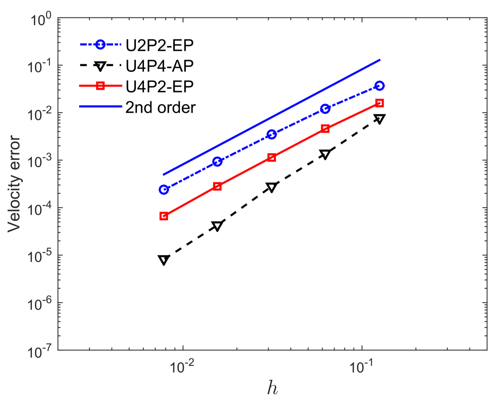
The Burggraf flow problem is adopted to test the numerical schemes under Dirichlet boundary conditions. Figure 3 shows the streamline pattern of the the Burggraf flow using the U4P4-AP formulation on a grid. Similar to the Taylor–Green vortices problem, the computation is also performed on five grids, i.e., , , , and . In Figure 4, the computation errors of x-velocity in the norm by different schemes are displayed against the spatial discretization size h. The velocity error by the U4P4-AP formulation is the smallest and the accuracy is between second order and third order. In comparison, both U2P2-EP and U4P2-EP have approximately second-order accuracy for velocity, and the error magnitude of U4P2-EP is smaller. The degradation of numerical accuracy is similar to the result of [48], in which only a second-order accuracy was obtained for the same problem, despite the use of a sixth-order compact scheme. They interpreted it by a second-order error due to the spectral treatment of the pressure through a cosine expansion.
3.3. Lid-Driven Cavity Flow
The lid-driven cavity flow is one of the most popular benchmark problems to test numerical methods for incompressible Navier–Stokes equations. This problem is quite similar to the Burggraf flow, except that the forcing term does not exist and the lid-velocity at the top boundary is uniform. In this case, the flow is also constrained in a square domain with the no-slip conditions for velocities at the bottom, left and right boundaries, and a slip velocity condition and at the top boundary, as well as Reynolds number . The computation is carried on a grid.
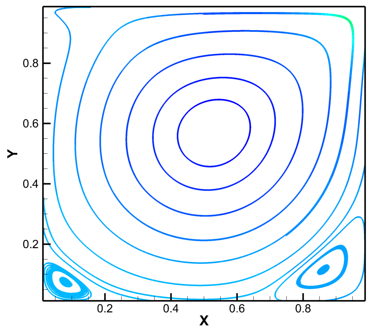
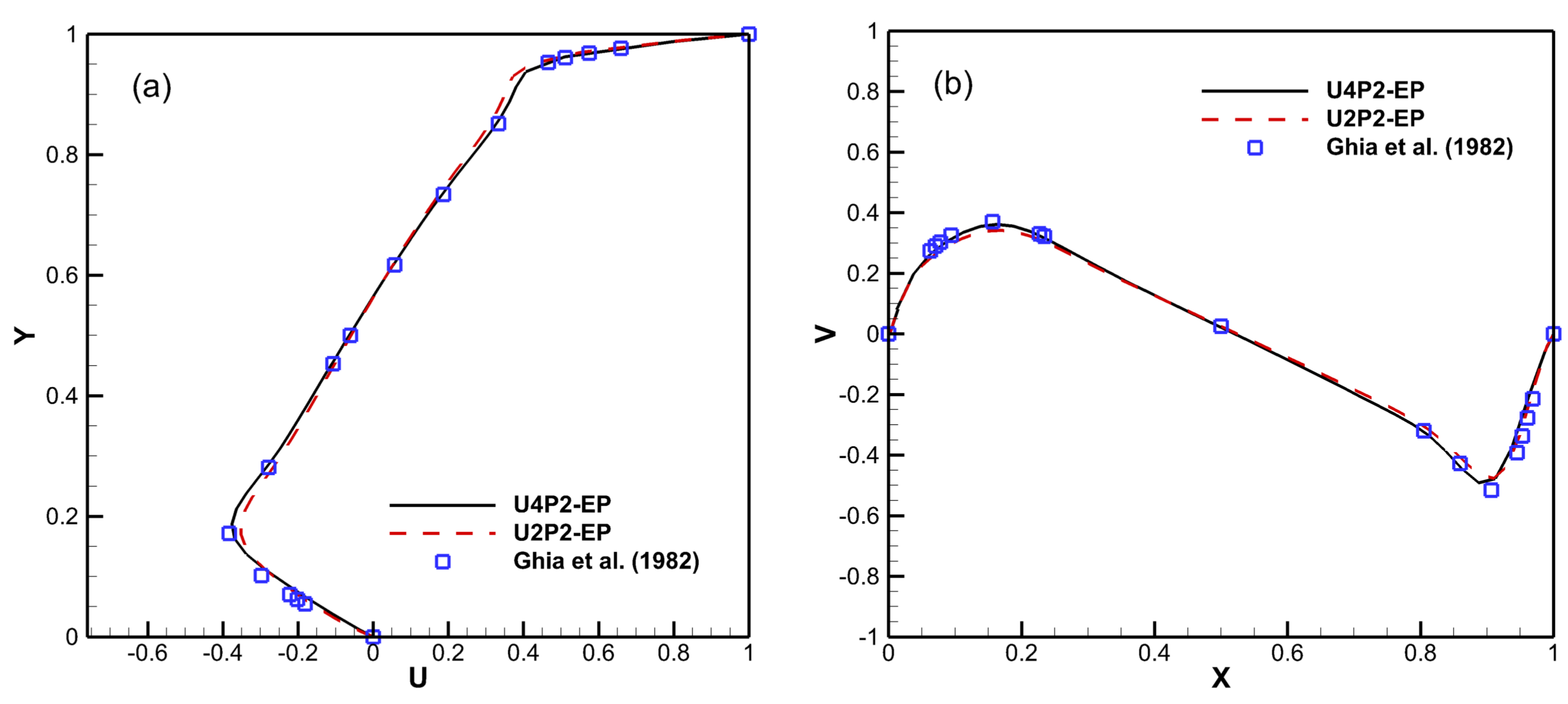
The computed streamline pattern is displayed in Figure 5, in which two corner circulation zones with unequal strength are observed. Velocity distributions by the present computation are compared with those obtained by [61], as shown in Figure 6. It is seen that, on a relatively coarse grid, the U4P2-EP formulation can produce more accurate predictions for velocity than the U2P2-EP formulation. This result is consistent with that of the Burggraf flow problem.
4. Computation of Turbulent Channel Flows
In this section, the proposed numerical method is applied in the computation of turbulent plane turbulent channel flows at low and high Reynolds numbers (, 590 and 1000) by DNS or LES. Several public DNS databases of channel flow by spectral method are available, thus comprehensive comparisons can be made. The definition of the friction Reynolds number is = , where = is the friction velocity, and are the average wall shear stress and fluid density respectively, H is the channel half height and is the kinematic viscosity of fluid. It is noted that the second-order central difference scheme is adopted in the vertical direction for all of the computations, since the grid is either stretched or it is much easier to be combined with a wall model.
4.1.
For the low-Reynolds number channel flow case, i.e., , comparisons are made with the spectral DNS database of [5]. We carried out DNS with second-order central difference scheme and fourth-order compact difference scheme separately without any turbulence model. The computational domain is and grid number is , the same as [5], in which x, y and z are the streamwise, vertical and spanwise directions, respectively. The grids in x- and z-directions are uniformly distributed with resolutions of and ; here, the superscript + indicates a variable normalized by the friction velocity and viscosity (wall units). The grid is stretched vertically by a hyperbolic tangential function, resulting in grid spacing of from walls to channel center. The flow in the x- and z-directions are periodic, as well as non-slip conditions at the upper and bottom walls.
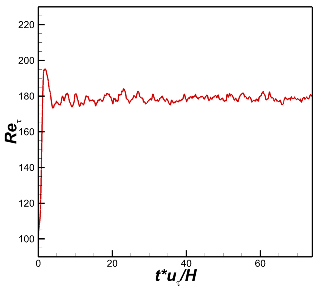
The simulation was performed for a long enough time to reach a statistically stationary state, as in Figure 7, over more than 70 non-dimensional time units. Plane- and time-averaged turbulence statistics and energy spectra are compared in the following. Figure 8 shows the mean streamwise velocity profile with respect to , in which MKM indicates the spectral DNS result of [5]. Present computation with the fourth-order compact difference DNS agrees well with MKM, while the result using the second-order central difference DNS slightly underestimates the streamwise velocity in the outer region. In Figure 9, the second-order turbulence statistics, like the root-mean-squared (r.m.s) values of velocity fluctuations and the tangential Reynolds stress, are displayed and compared. It is seen that both the second- and fourth-order schemes yield accurate predictions of the second-order moments. Figure 10 shows the one-dimensional streamwise pre-multiplied spectra at two heights, i.e., and . The peaks of the pre-multiplied spectra correspond to the length scale of the most energetic turbulent coherent structures, which are as the typical length scale of the near-wall streaks [62]. The differences between the results of the second- and fourth-order methods are obvious. The shapes and peaks of the spectra via the central difference DNS are shifted to smaller length scales, while better agreements have been obtained with the compact difference scheme. This may be explained by the large dispersion errors of the second-order scheme in high wavenumber (small scale) regime.
4.2.
We also performed large-eddy simulation study of turbulent channel flow at . In LES, the filtered Navier–Stokes equations
are solved, where is filtered variable and is the subgrid-scale (SGS) or the residual stresses. The dynamic Smagorinsky model [63,64] for SGS stresses is adopted, as well as a box filter in the plane using the Simpson’s rule for test filtering. Recently, Xie et al. [65] have demonstrated that the box filter is superior to the Gaussian filter when combined with FD-LES. In addition to the explicit SGS modeling approach adopted here, the implicit large-eddy simulation methodology combined with high-order numerical schemes are also under notable development [66,67,68,69,70].
The computation domain size is , the same as [5], and the grid is . The grid distributions are uniform in x- and z-directions with and , and stretched in the y-direction with from wall to channel center.
Results are displayed in Figure 11, Figure 12 and Figure 13. In general, the mean streamwise velocity, velocity fluctuations and tangential Reynolds stress by LES with the fourth-order compact scheme coincide well with the spectral DNS, slightly better than the second-order central difference scheme, as displayed in Figure 11 and Figure 12. The mean streamwise velocity is underestimated in the outer layer, and the streamwise velocity fluctuation is a little overestimated in the inner layer but underestimated in the outer layer by the low-order scheme. Furthermore, the peaks of one-dimensional streamwise premultiplied spectra are obviously overestimated by a central difference scheme in the buffer layer; in comparison, the results of compact difference LES are more reasonable, which are depicted in Figure 13.
4.3.
Next, we move to a higher Reynolds number, i.e., , as the last case. Wall-modeled large-eddy simulation [71,72], or WMLES for short, with an equilibrium wall stress model [73,74] is adopted. The wall model relates the average flow velocity near the wall and the average wall stress through the classical logarithmic law, which is
Here, is the average total velocity parallel to the wall at (the jth grid in wall normal direction), and we chose following the suggestions of [75,76]. The von Kármán constant and . Equation (54) is solved iteratively by the Newton–Rampson method to obtain the friction velocity and thus the total average wall stress . In addition, the wall stress components in x- and z-directions are obtained by
Thus, in the WMLES, the filtered Navier–Stokes equations are coupled with wall stress boundary conditions in x- and z-directions.
The computation is compared with a recent spectral DNS study of high Reynolds number channel flows up to [9]. The domain size is (half channel), which is the same as [9] in streamwise and spanwise. The grid is with uniform distributions in all three directions. The grid size is thus approximately in x- and z-directions. This grid resolution is much coarser than [77] for accurately reproducing the generalized logarithmic law for high-order moments of a high Reynolds number wall turbulent flow, in which the finest grid resolution is less than , but similar to the resolution used by [78].
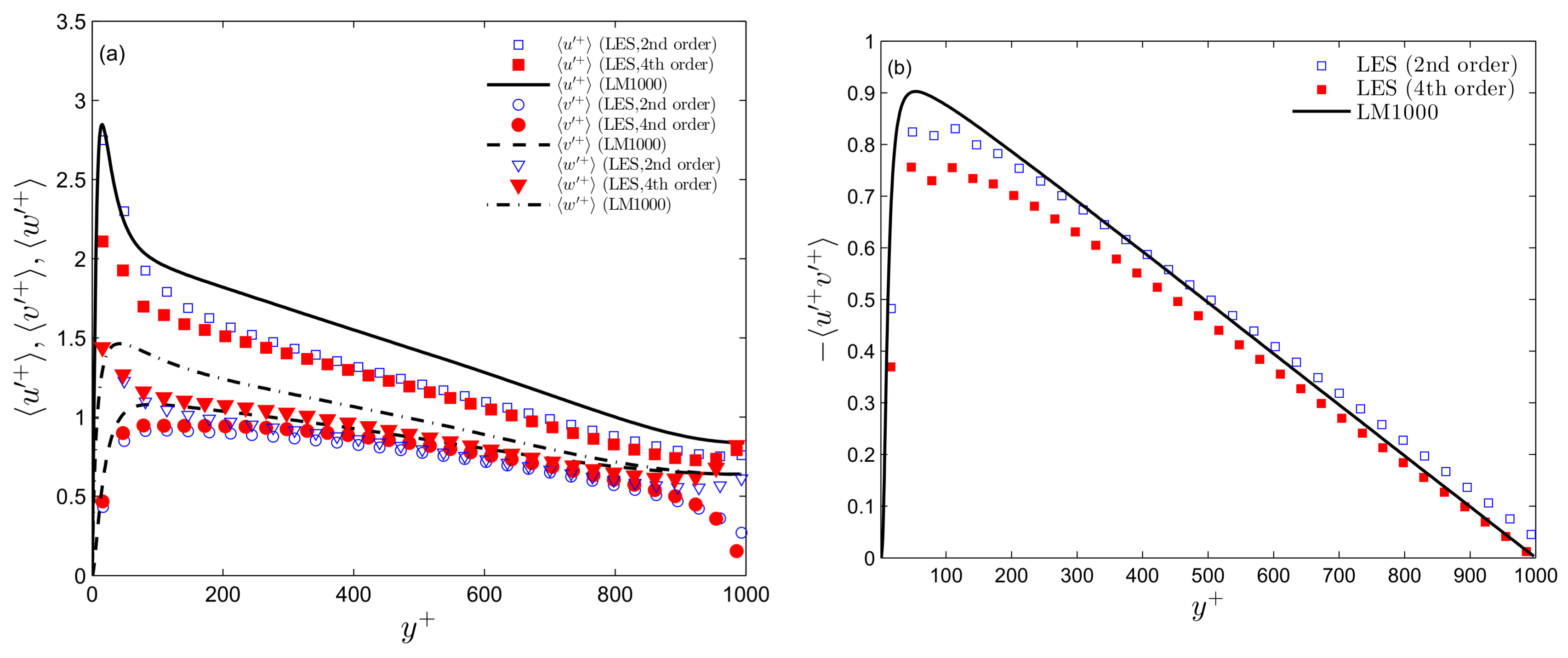
Figure 14 displays the mean streamwise velocity obtained by WMLES as well as the DNS result of [9] (indicated by LM1000) for comparison. The first vertical grid of WMLES is located in the buffer layer, hence it deviates from the DNS result. Above the buffer layer, the mean streamwise velocity profile computed via the compact difference agrees well with LM1000, while it is obviously underestimated by the central difference scheme. The velocity fluctuations and tangential Reynolds stress are shown in Figure 15. Generally, the predictions by the low-order scheme are a little larger than those by the high-order scheme. However, it does not mean that the low-order one is better, since the grid is quite coarse so that the resolved turbulent kinetic energy and Reynolds stress should be smaller than the total quantities to a certain content.
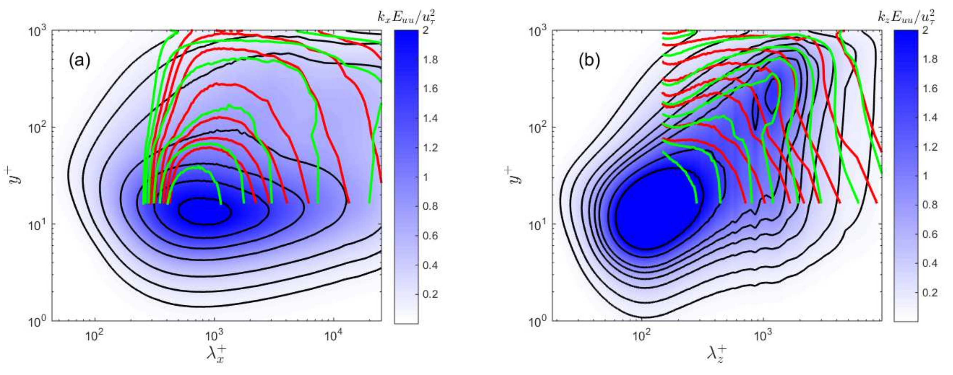
The two-dimensional premultiplied spectrogram is a contour plot of one-dimensional premultiplied spectra along the vertical direction to demonstrate turbulent energy distribution in both wavelength and wall normal distance. The streamwise and spanwise premultiplied spectrograms and are plotted in Figure 16. In the logarithmic region and sufficiently large length scales, the WMLES using a high-order compact difference scheme can predict more energetic spectral densities, which agrees better with DNS (LM1000) than the second-order central difference scheme.
5. Discussion
A numerical method for solving the incompressible Navier–Stokes equations efficiently with a semi-implicit time advancement on a fully staggered grid using a high-order compact difference scheme was developed in the framework of approximate factorization. A fourth-order compact difference scheme was adopted for approximations of derivatives and interpolations of the flow equations. The pressure Poisson equation was directly solved by the Fourier transform method. Since the Poisson equation is the most time-consuming step, the present method should be much more efficient than iterative solvers, although we did not show any direct evidence. For temporal advancement, in addition to the explicit Adams–Bashforth scheme for convection terms, the semi-implicit Crank–Nicolson scheme was used for viscous terms to permit a large time step. Currently, the code is parallelised by OpenMP.
The present numerical method has been tested and validated in several benchmark problems, including the Taylor–Green vortices, Burggraf flow and lid-driven cavity flow. It was shown that high-order accuracy could be achieved. In the last part of the study, we preliminarily applied the present numerical method to the computation of turbulent channel flows at low and high Reynolds numbers by DNS and LES. In comparison with the second-order central difference scheme, it was found that the predictions of turbulence statistics and especially spectra could be obviously improved by using the high-order compact difference scheme. To the authors’ knowledge, there is little work like the present comprehensive tests of high-order compact scheme in computation of low and moderate Reynolds number wall-bounded turbulent flows.
It should be further noted that, for non-periodic problems, the present numerical method is not fourth-order accurate, whereas the U4P4-AP formulation is between second- and third-order accurate, and its numerical error is absolutely smaller than the classic second-order central difference scheme. In addition, in the computation of turbulent channel flows, the second-order central difference scheme is used in the vertical direction, thus the overall numerical method should not be fourth order. However, benefits of using a high-order scheme in the homogeneous directions are quite obvious from our results, especially for the turbulence energy spectra. In addition, through DNS studies of [79], it was found that low order statistics of turbulence may not necessarily be improved via a high-order compact difference scheme, while only higher-order statistics and spectra can be improved. This result is consistent with the present work, in which the different numerical schemes only have marginal effects on the the low order statistics in the well-resolved DNS or LES simulations because the resolutions are fine enough to capture the most energetic eddies in turbulence. However, for WMLES with a coarse resolution, the numerical errors may play a role, which can be in the same order of magnitude with the SGS stresses [17], and the adoption of a high-order scheme should be necessary.
Acknowledgments
The financial support by grants from the National Natural Science Foundation of China (11502185, 11490553, 91752107 and 11362010), the Natural Science Basic Research Plan in Shaanxi Province of China (2016JQ1004) and the Key Laboratory of Mechanics on Disaster and Environment in Western China (Klmwde201501) are gratefully acknowledged. The computation was partly performed at the HPC center of Xidian University and Tianhe-2 supercomputer at the National Supercomputer Center in Guangzhou.
Author Contributions
R.H. and L.W. conceived and designed the numerical method; R.H., L.W. and P.W. performed the simulations; R.H., L.W., P.W. and Y.W. analyzed the data; R.H. and X.Z. wrote the paper.
Conflicts of Interest
The authors declare no conflict of interest. The founding sponsors had no role in the design of the study; in the collection, analyses, or interpretation of data; in the writing of the manuscript, and in the decision to publish the results.
Abbreviations
The following abbreviations are used in this manuscript:
| AP | Approximate Projection |
| CFD | Computational Fluid Dynamics |
| DCT | Discrete Cosine Transform |
| DFT | Discrete Fourier Transform |
| DNS | Direct Numerical Simulation |
| EP | Exact Projection |
| FD | Finite Difference |
| FFT | Fast Fourier Transform |
| FV | Finite Volume |
| HPC | High Performance Computation |
| LES | Large Eddy Simulation |
| LM | Lee and Moser |
| MKM | Moser, Kim and Mansour |
| R.m.s | Root-mean-squared |
| SIMPLE | Semi-Implicit Method for Pressure-Linked Equations |
| WMLES | Wall-Modeled Large Eddy Simulation |
References
- Lesieur, M.; Metais, O. New trends in large-eddy simulations of turbulence. Annu. Rev. Fluid Mech. 1996, 28, 45–82. [Google Scholar] [CrossRef]
- Moin, P.; Mahesh, K. Direct numerical simulation: A tool in turbulence research. Annu. Rev. Fluid Mech. 1998, 30, 539–578. [Google Scholar] [CrossRef]
- Meneveau, C.; Katz, J. Scale-invariance and turbulence models for large-eddy simulation. Annu. Rev. Fluid Mech. 2000, 32, 1–32. [Google Scholar] [CrossRef]
- Kim, J.; Moin, P.; Moser, R. Turbulence statistics in fully developed channel flow at low Reynolds number. J. Fluid Mech. 1987, 177, 133–166. [Google Scholar] [CrossRef]
- Moser, R.; Kim, J.; Mansour, M.N. Direct numerical simulation of turbulent channel flow up to Reτ = 590. Phys. Fluids 1999, 11, 943–945. [Google Scholar] [CrossRef]
- Del Álamo, J.C.; Jiménez, J.; Zandonade, P.; Moser, R.D. Scaling of the energy spectra of turbulent channels. J. Fluid Mech. 2004, 500, 135–144. [Google Scholar] [CrossRef]
- Hoyas, S.; Jiménez, J. Scaling of the velocity fluctuations in turbulent channels up to Reτ = 2003. Phys. Fluids 2006, 18, 011702. [Google Scholar] [CrossRef]
- Lozano-Durán, A.; Jiménez, J. Effect of the computational domain on direct simulations of turbulent channels up to Reτ = 4200. Phys. Fluids 2014, 26, 011702. [Google Scholar] [CrossRef]
- Lee, M.; Moser, R.D. Direct numerical simulation of turbulent channel flow up to Reτ ≈ 5200. J. Fluid Mech. 2015, 774, 943–945. [Google Scholar] [CrossRef]
- Wu, X.; Moin, P. A direct numerical simulation study on the mean velocity characteristics in turbulent pipe flow. J. Fluid Mech. 2008, 608, 81–112. [Google Scholar] [CrossRef]
- Chin, C.; Monty, J.P.; Ooi, A. Reynolds number effects in DNS of pipe flow and comparison with channels and boundary layers. Int. J. Heat Fluid Flow 2014, 45, 33–40. [Google Scholar] [CrossRef]
- Wu, X.; Moin, P.; Adrian, R.J.; Baltzer, J.R. Osborne Reynolds pipe flow: Direct simulation from laminar through gradual transition to fully developed turbulence. Proc. Natl. Acad. Sci. USA 2015, 112, 7920–7924. [Google Scholar] [CrossRef] [PubMed]
- Ahn, J.; Lee, J.H.; Jin, L.; Kang, J.; Sung, H.J. Direct numerical simulation of a 30R long turbulent pipe flow at Reτ = 3008. Phys. Fluids 2015, 27, 065110. [Google Scholar] [CrossRef]
- Harlow, F.H.; Welch, J.E. Numerical calculation of time-dependent viscous incompressible flow of fluid with free surface. Phys. Fluids 1965, 8, 2182–2189. [Google Scholar] [CrossRef]
- Bernardini, M.; Pirozzoli, S.; Orlandi, P. Velocity statistics in turbulent channel flow up to Reτ = 4000. J. Fluid Mech. 2014, 742, 171–191. [Google Scholar] [CrossRef]
- Moin, P.; Verzicco, R. On the suitability of second-order accurate discretizations for turbulent flow simulations. Eur. J. Mech. B/Fluids 2016, 55, 242–245. [Google Scholar] [CrossRef]
- Kravchenko, A.G.; Moin, P. On the effect of numerical errors in large eddy simulations of turbulent flows. J. Comput. Phys. 1997, 131, 310–322. [Google Scholar] [CrossRef]
- Morinishi, Y.; Lund, T.S.; Vasilyev, O.V.; Moin, P. Fully conservative higher order finite difference schemes for incompressible flow. J. Comput. Phys. 1998, 143, 90–124. [Google Scholar] [CrossRef]
- Verstappen, R.W.C.P.; Veldman, A.E.P. Symmetry-preserving discretization of turbulent flow. J. Comput. Phys. 2003, 187, 343–368. [Google Scholar] [CrossRef]
- Lele, S.K. Compact finite difference schemes with spectral-like resolution. J. Comput. Phys. 1992, 103, 16–42. [Google Scholar] [CrossRef]
- Mahesh, K. A family of high order finite difference schemes with good spectral resolution. J. Comput. Phys. 1998, 145, 332–358. [Google Scholar] [CrossRef]
- Deng, X.; Zhang, H. Developing high-order weighted compact nonlinear schemes. J. Comput. Phys. 2000, 165, 22–44. [Google Scholar] [CrossRef]
- Nagarajan, S.; Lele, S.K.; Ferziger, J.H. A robust high-order compact method for large eddy simulation. J. Comput. Phys. 2003, 191, 392–419. [Google Scholar] [CrossRef]
- Zhou, Q.; Yao, Z.; He, F.; Shen, M. A new family of high-order compact upwind difference schemes with good spectral resolution. J. Comput. Phys. 2007, 227, 1306–1339. [Google Scholar] [CrossRef]
- Rizzetta, D.P.; Visbal, M.R.; Morgan, P.E. A high-order compact finite-difference scheme for large-eddy simulation of active flow control. Prog. Aerosp. Sci. 2008, 44, 397–426. [Google Scholar] [CrossRef]
- Zhang, S.; Jiang, S.; Shu, C.W. Development of nonlinear weighted compact schemes with increasingly higher order accuracy. J. Comput. Phys. 2008, 227, 7294–7321. [Google Scholar] [CrossRef]
- Patankar, S. Numerical Heat Transfer and Fluid Flow; CRC Press: Boca Raton, FL, USA, 1980. [Google Scholar]
- Patankar, S.V.; Spalding, D.B. A calculation procedure for heat, mass and momentum transfer in three-dimensional parabolic flows. In Numerical Prediction of Flow, Heat Transfer, Turbulence and Combustion; Elsevier: Amsterdam, The Netherlands, 1983; pp. 54–73. [Google Scholar]
- Van Doormaal, J.; Raithby, G. Enhancements of the SIMPLE method for predicting incompressible fluid flows. Numer. Heat Transf. 1984, 7, 147–163. [Google Scholar] [CrossRef]
- Kwak, D.; Chang, J.L.; Shanks, S.P.; Chakravarthy, S.R. A three-dimensional incompressible Navier–Stokes flow solver using primitive variables. AIAA J. 1986, 24, 390–396. [Google Scholar] [CrossRef]
- Drikakis, D.; Govatsos, P.; Papantonis, D. A characteristic-based method for incompressible flows. Int. J. Numer. Methods Fluids 1994, 19, 667–685. [Google Scholar] [CrossRef]
- Shapiro, E.; Drikakis, D. Artificial compressibility, characteristics-based schemes for variable density, incompressible, multi-species flows. Part I: Derivation of different formulations and constant density limit. J. Comput. Phys. 2005, 210, 584–607. [Google Scholar] [CrossRef] [Green Version]
- Chorin, A.J. Numerical solution of Navier-Stokes equations. Math. Comput. 1968, 22, 745–762. [Google Scholar] [CrossRef]
- Janenko, N.N. The Method of Fractional Steps; Springer: Berlin, Germany, 1971. [Google Scholar]
- Kim, J.; Moin, P. Application of a fractional-step method to incompressible Navier-Stokes equations. J. Comput. Phys. 1985, 59, 308–323. [Google Scholar] [CrossRef]
- Van Kan, J. A second-order accurate pressure-correction scheme for viscous incompressible flow. SIAM J. Sci. Stat. Comput. 1986, 7, 870–891. [Google Scholar] [CrossRef]
- Bell, J.B.; Colella, P.; Glaz, H.M. A second-order projection method for the incompressible Navier-Stokes equations. J. Comput. Phys. 1989, 85, 257–283. [Google Scholar] [CrossRef]
- Brown, D.L.; Cortez, R.; Minion, M.L. Accurate projection methods for the incompressible Navier-Stokes equations. J. Comput. Phys. 2001, 168, 464–499. [Google Scholar] [CrossRef]
- Drikakis, D.; Rider, W. High-Resolution Methods for Incompressible and Low-Speed Flows; Springer Science & Business Media: Berlin/Heidelberg, Germany, 2006. [Google Scholar]
- Ferziger, J.H.; Peric, M. Computational Methods for Fluid Dynamics; Springer Science & Business Media: New York, NY, USA, 2012. [Google Scholar]
- Ma, Y.; Fu, D.; Kobayashi, T.; Taniguchi, N. Numerical solution of the incompressible Navier–Stokes equations with an upwind compact difference scheme. Int. J. Numer. Methods Fluids 1999, 30, 509–521. [Google Scholar]
- Demuren, A.O.; Wilson, R.V.; Carpenter, M. Higher-order compact schemes for numerical simulation of incompressible flows, Part I: Theoretical development. Numer. Heat Transf. Part B Fundam. 2001, 39, 207–230. [Google Scholar]
- Wilson, R.V.; Demuren, A.O.; Carpenter, M. Higher-order compact schemes for numerical simulation of incompressible flows, part II: Applications. Numer. Heat Transf. Part B Fundam. 2001, 39, 231–255. [Google Scholar]
- Abide, S.; Viazzo, S. A 2D compact fourth-order projection decomposition method. J. Comput. Phys. 2005, 206, 252–276. [Google Scholar] [CrossRef]
- Zhang, K.K.; Shotorban, B.; Minkowycz, W.; Mashayek, F. A compact finite difference method on staggered grid for Navier–Stokes flows. Int. J. Numer. Methods Fluids 2006, 52, 867–881. [Google Scholar] [CrossRef]
- Pandit, S.K.; Kalita, J.C.; Dalal, D. A transient higher order compact scheme for incompressible viscous flows on geometries beyond rectangular. J. Comput. Phys. 2007, 225, 1100–1124. [Google Scholar] [CrossRef]
- Knikker, R. Study of a staggered fourth-order compact scheme for unsteady incompressible viscous flows. Int. J. Numer. Methods Fluids 2009, 59, 1063–1092. [Google Scholar] [CrossRef]
- Laizet, S.; Lamballais, E. High-order compact schemes for incompressible flows: A simple and efficient method with quasi-spectral accuracy. J. Comput. Phys. 2009, 228, 5989–6015. [Google Scholar] [CrossRef]
- Boersma, B.J. A 6th order staggered compact finite difference method for the incompressible Navier–Stokes and scalar transport equations. J. Comput. Phys. 2011, 230, 4940–4954. [Google Scholar] [CrossRef]
- Tyliszczak, A. A high-order compact difference algorithm for half-staggered grids for laminar and turbulent incompressible flows. J. Comput. Phys. 2014, 276, 438–467. [Google Scholar] [CrossRef]
- Reis, G.A.; Tasso, I.V.M.; Souza, L.F.; Cuminato, J.A. A compact finite differences exact projection method for the Navier-Stokes equations on a staggered grid with fourth-order spatial precision. Comput. Fluids 2015, 118, 19–31. [Google Scholar] [CrossRef]
- Sengupta, T.K.; Sengupta, A. A new alternating bi-diagonal compact scheme for non-uniform grids. J. Comput. Phys. 2016, 310, 1–25. [Google Scholar] [CrossRef]
- Abide, S.; Binous, M.; Zeghmati, B. An efficient parallel high-order compact scheme for the 3D incompressible Navier-Stokes equations. Int. J. Comput. Fluid Dyn. 2017, 1–16. [Google Scholar] [CrossRef]
- Dukowicz, J.K.; Dvinsky, A.S. Approximate factorisation as a high order splitting for the incompressible flow equations. J. Comput. Phys. 1992, 102, 336–347. [Google Scholar] [CrossRef]
- Perot, J.B. An analysis of the fractional step method. J. Comput. Phys. 1993, 108, 51–58. [Google Scholar] [CrossRef]
- Kim, K.; Baek, S.J.; Sung, H.J. An implicit velocity decoupling procedure for the incompressible Navier-Stokes equations. Int. J. Numer. Methods Fluids 2002, 38, 125–138. [Google Scholar] [CrossRef]
- Orszag, S.A.; Israeli, M.; Deville, M.O. Boundary conditions for incompressible flows. J. Comput. Phys. 1986, 1, 75–111. [Google Scholar] [CrossRef]
- Gresho, P.M.; Sani, R.L. On pressure boundary conditions for the incompressible Navier–Stokes equations. Int. J. Numer. Methods Fluids 1987, 7, 1111–1145. [Google Scholar] [CrossRef]
- Makhoul, J. A fast cosine transform in one and two dimensions. IEEE Trans. Acoust. Speech Signal Proc. 1980, 28, 27–34. [Google Scholar] [CrossRef]
- Shih, T.M.; Tan, C.H.; Hwang, B.C. Effects of grid staggering on numerical schemes. Int. J. Numer. Methods Fluids 1989, 9, 193–212. [Google Scholar] [CrossRef]
- Ghia, U.; Ghia, K.N.; Shin, C.T. High-Re solutions for incompressible flow using the Navier-Stokes equations and a multigrid method. J. Comput. Phys. 1982, 48, 387–411. [Google Scholar] [CrossRef]
- Pope, S.B. Turbulent Flows; Cambridge University Press: Cambridge, UK, 2000. [Google Scholar]
- Germano, M.; Piomelli, U.; Moin, P.; Cabot, W.H. A dynamic subgrid-scale eddy viscosity model. Phys. Fluids A Fluid Dyn. 1991, 3, 1760–1765. [Google Scholar] [CrossRef]
- Lilly, D.K. A proposed modification of the Germano subgrid-scale closure method. Phys. Fluids A Fluid Dyn. 1992, 4, 633–635. [Google Scholar] [CrossRef]
- Xie, S.; Ghaisas, N.; Archer, C.L. Sensitivity issues in finite-difference large-eddy simulations of the atmospheric boundary layer with dynamic subgrid-scale models. Bound. Layer Meteorol. 2015, 157, 421–445. [Google Scholar] [CrossRef]
- Boris, J.; Grinstein, F.; Oran, E.; Kolbe, R. New insights into large eddy simulation. Fluid Dyn. Res. 1992, 10, 199–228. [Google Scholar] [CrossRef]
- Margolin, L.; Rider, W.; Grinstein, F. Modeling turbulent flow with implicit LES. J. Turbul. 2006, N15. [Google Scholar] [CrossRef]
- Hickel, S.; Adams, N. On implicit subgrid-scale modeling in wall-bounded flows. Phys. Fluids 2007, 19, 105106. [Google Scholar] [CrossRef]
- Kokkinakis, I.; Drikakis, D. Implicit large eddy simulation of weakly-compressible turbulent channel flow. Comput. Methods Appl. Mech. Eng. 2015, 287, 229–261. [Google Scholar] [CrossRef] [Green Version]
- Tsoutsanis, P.; Kokkinakis, I.W.; Könözsy, L.; Drikakis, D.; Williams, R.J.; Youngs, D.L. Comparison of structured-and unstructured-grid, compressible and incompressible methods using the vortex pairing problem. Comput. Methods Appl. Mech. Eng. 2015, 293, 207–231. [Google Scholar] [CrossRef] [Green Version]
- Piomelli, U. Wall-layer models for large-eddy simulations. Annu. Rev. Fluid Mech. 2002, 34, 349–374. [Google Scholar] [CrossRef]
- Piomelli, U. Wall-layer models for large-eddy simulations. Prog. Aerosp. Sci. 2008, 44, 437–446. [Google Scholar] [CrossRef]
- Schumann, U. Subgrid-scale model for finite difference simulation of turbulent flows in plane channels and annuli. J. Comput. Phys. 1975, 18, 376–404. [Google Scholar] [CrossRef] [Green Version]
- Grötzbach, G. Encyclopedia of Fluid Mechanics; Chapter Direct Numerical and Large Eddy Simulations of Turbulent Channel Flows; Gulf Publishing Company: Houston, TX, USA, 1987; Volume 6, pp. 1337–1391. [Google Scholar]
- Kawai, S.; Larsson, J. Wall-modeling in large eddy simulation: Length scales, grid resolution, and accuracy. Phys. Fluids 2012, 24, 015105. [Google Scholar] [CrossRef]
- Lee, J.; Cho, M.; Choi, H. Large eddy simulations of turbulent channel and boundary layer flows at high Reynolds number with mean wall shear stress boundary condition. Phys. Fluids 2013, 25, 110808. [Google Scholar] [CrossRef]
- Stevens, R.J.A.M.; Wilczek, M.; Meneveau, C. Large-eddy simulation study of the logarithmic law for second- and higher-order moments in turbulent wall-bounded flow. J. Fluid Mech. 2014, 757, 888–907. [Google Scholar] [CrossRef]
- Chung, D.; McKeon, B.J. Large-eddy simulation of large-scale structures in long channel flow. J. Fluid Mech. 2010, 661, 341–364. [Google Scholar] [CrossRef]
- Suzuki, H.; Nagata, K.; Sakai, Y.; Hayase, T.; Hasegawa, Y.; Ushijima, T. An attempt to improve accuracy of higher-order statistics and spectra in direct numerical simulation of incompressible wall turbulence by using the compact schemes for viscous terms. Int. J. Numer. Methods Fluids 2013, 73, 509–522. [Google Scholar] [CrossRef]
Figure 1.
The streamline pattern of the Taylor–Green vortices problem at computed by using the 4th-order compact difference scheme on the grid, with coloring by pressure magnitude.
Figure 1.
The streamline pattern of the Taylor–Green vortices problem at computed by using the 4th-order compact difference scheme on the grid, with coloring by pressure magnitude.
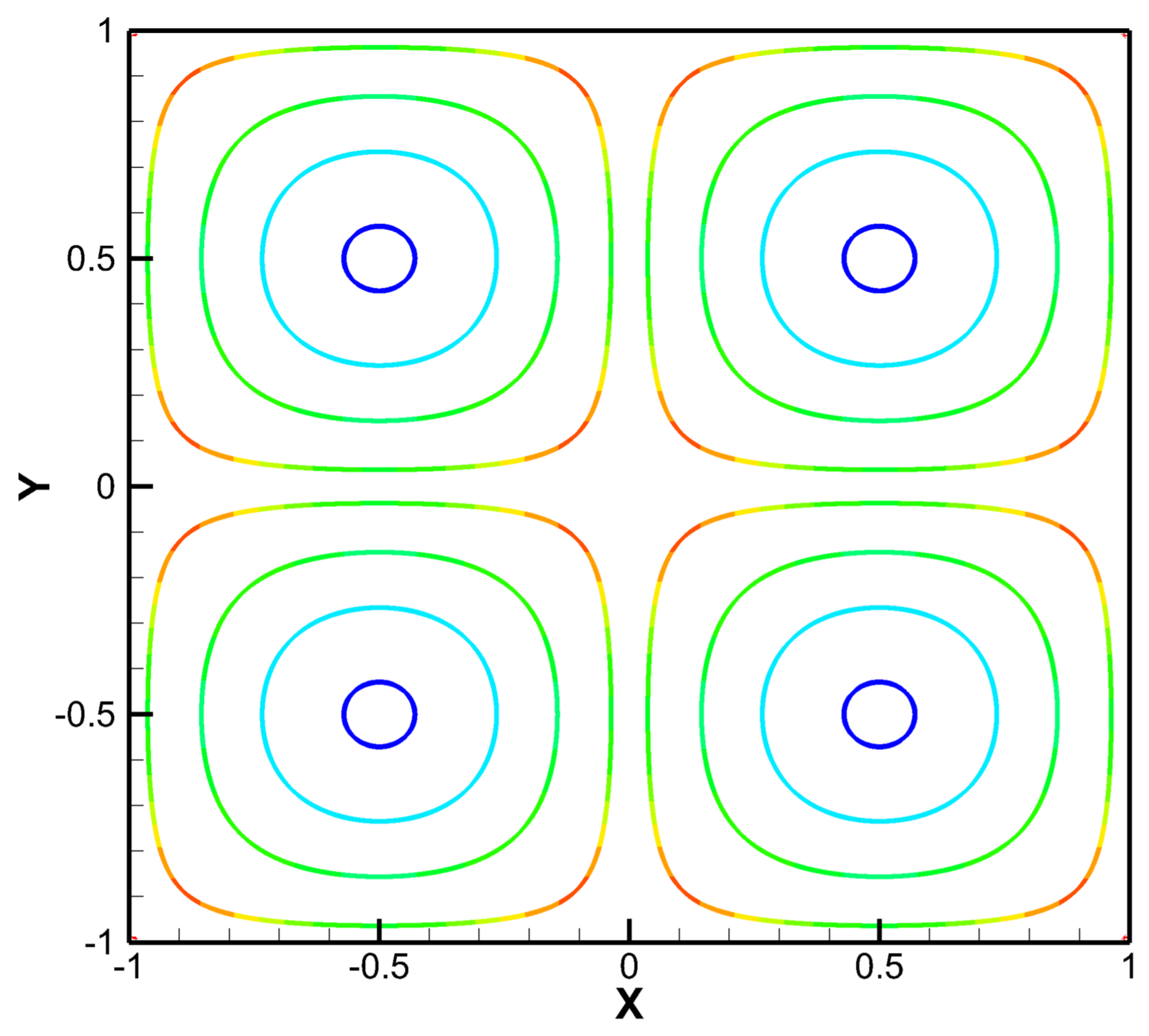
Figure 2.
Computation errors ( norm) of the Taylor–Green vortices problem. Left: x-velocity error with the spatial discretization size. Right: pressure error with the spatial discretization size.
Figure 2.
Computation errors ( norm) of the Taylor–Green vortices problem. Left: x-velocity error with the spatial discretization size. Right: pressure error with the spatial discretization size.
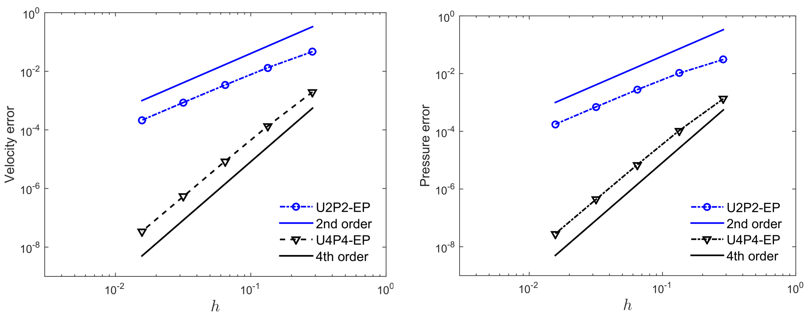
Figure 3.
The streamline pattern of the Burggraf flow problem computed by using the U4P4-AP formulation on the grid.
Figure 3.
The streamline pattern of the Burggraf flow problem computed by using the U4P4-AP formulation on the grid.
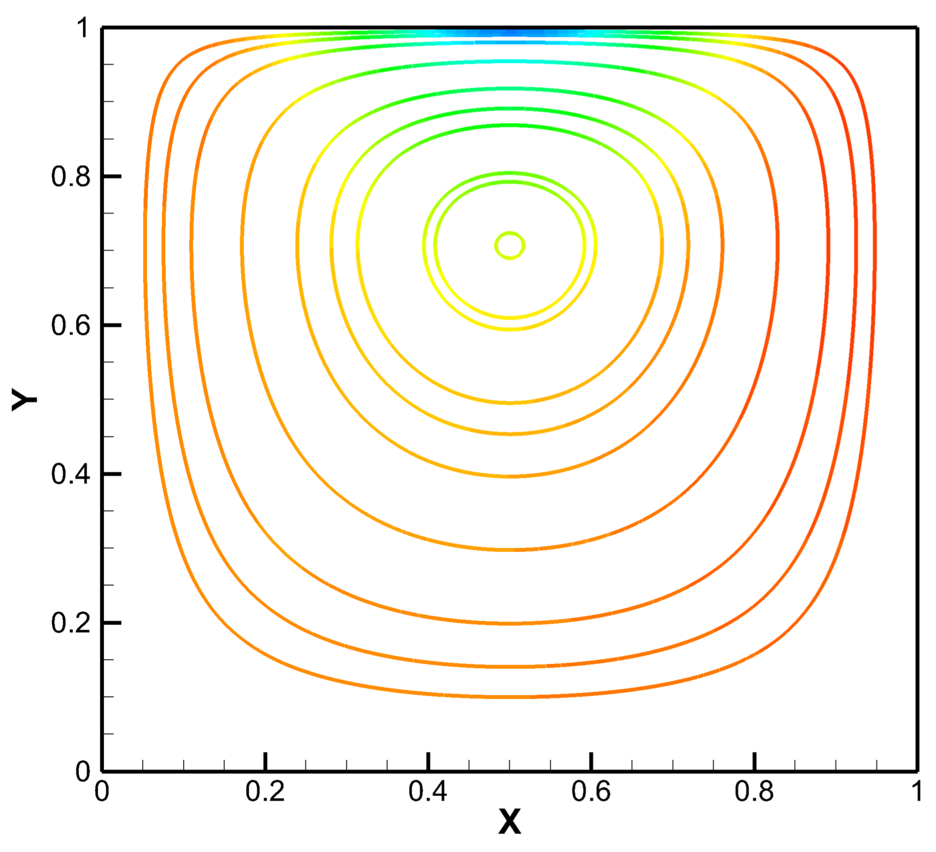
Figure 4.
Computation errors ( norm) of x-velocity error in the Burggraf flow problem.

Figure 5.
The streamline pattern of the Burggraf flow problem computed by using the U4P2-EP formulation on a grid.
Figure 5.
The streamline pattern of the Burggraf flow problem computed by using the U4P2-EP formulation on a grid.

Figure 6.
Comparison of (a) horizontal and (b) vertical velocity components at the vertical and horizontal centerlines with reference data of [61]. Upper: x-velocity. Lower: y-velocity.
Figure 6.
Comparison of (a) horizontal and (b) vertical velocity components at the vertical and horizontal centerlines with reference data of [61]. Upper: x-velocity. Lower: y-velocity.

Figure 7.
Time histories of friction Reynolds number at by DNS.

Figure 8.
Mean streamwise velocity of turbulent channel flow at by DNS.
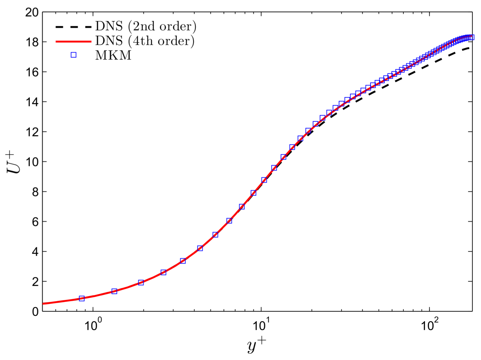
Figure 9.
(a) R.m.s of velocity fluctuations and (b) tangential Reynolds stress of turbulent channel flow at by DNS.
Figure 9.
(a) R.m.s of velocity fluctuations and (b) tangential Reynolds stress of turbulent channel flow at by DNS.
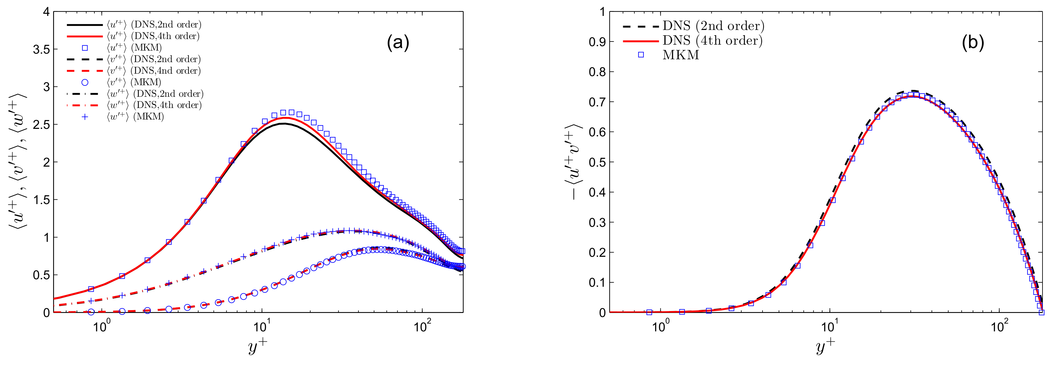
Figure 10.
One-dimensional streamwise pre-multiplied spectra at (a) and (b) ≈ 30 of turbulent channel flow at by DNS.
Figure 10.
One-dimensional streamwise pre-multiplied spectra at (a) and (b) ≈ 30 of turbulent channel flow at by DNS.
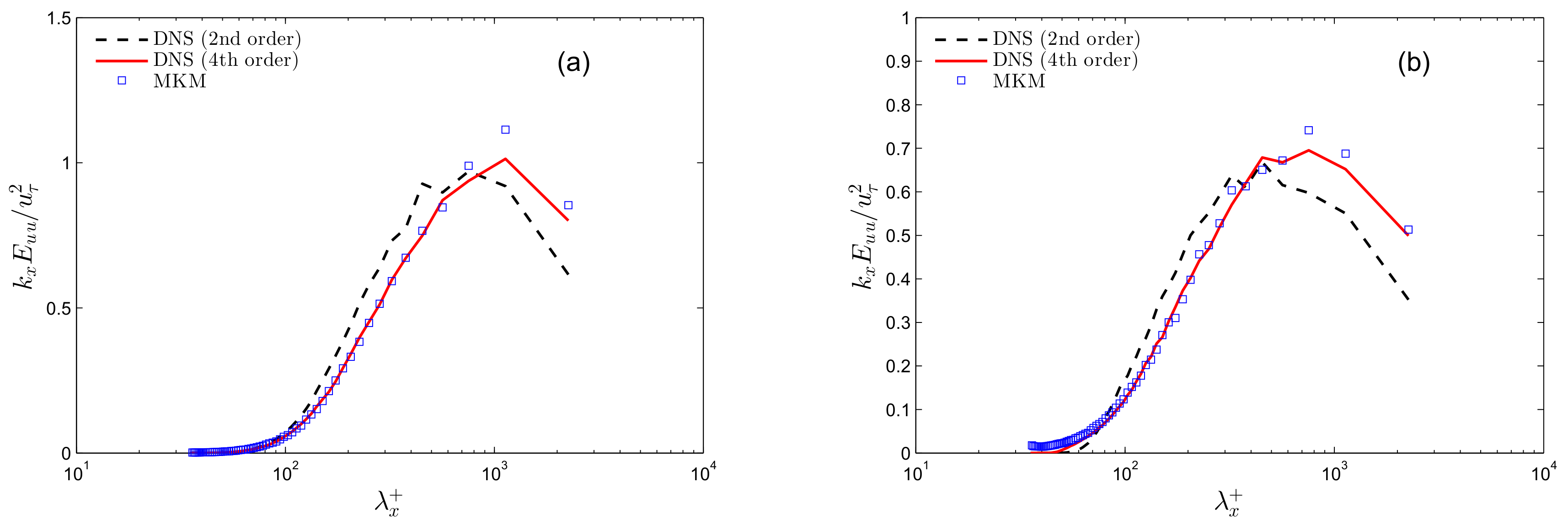
Figure 11.
Mean streamwise velocity of turbulent channel flow by LES at .
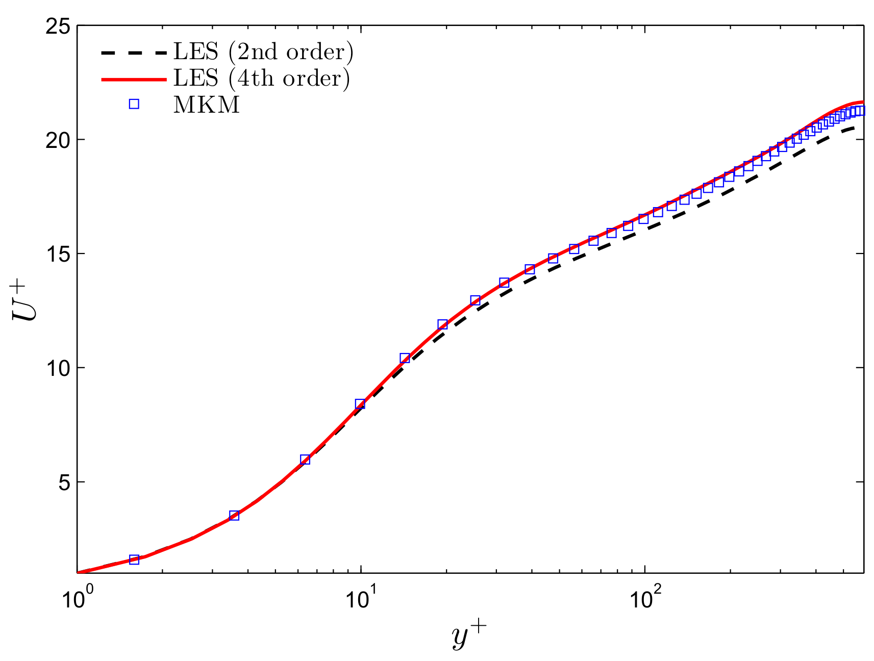
Figure 12.
(a) R.m.s of velocity fluctuations and (b) tangential Reynolds stress of turbulent channel flow by LES at .
Figure 12.
(a) R.m.s of velocity fluctuations and (b) tangential Reynolds stress of turbulent channel flow by LES at .
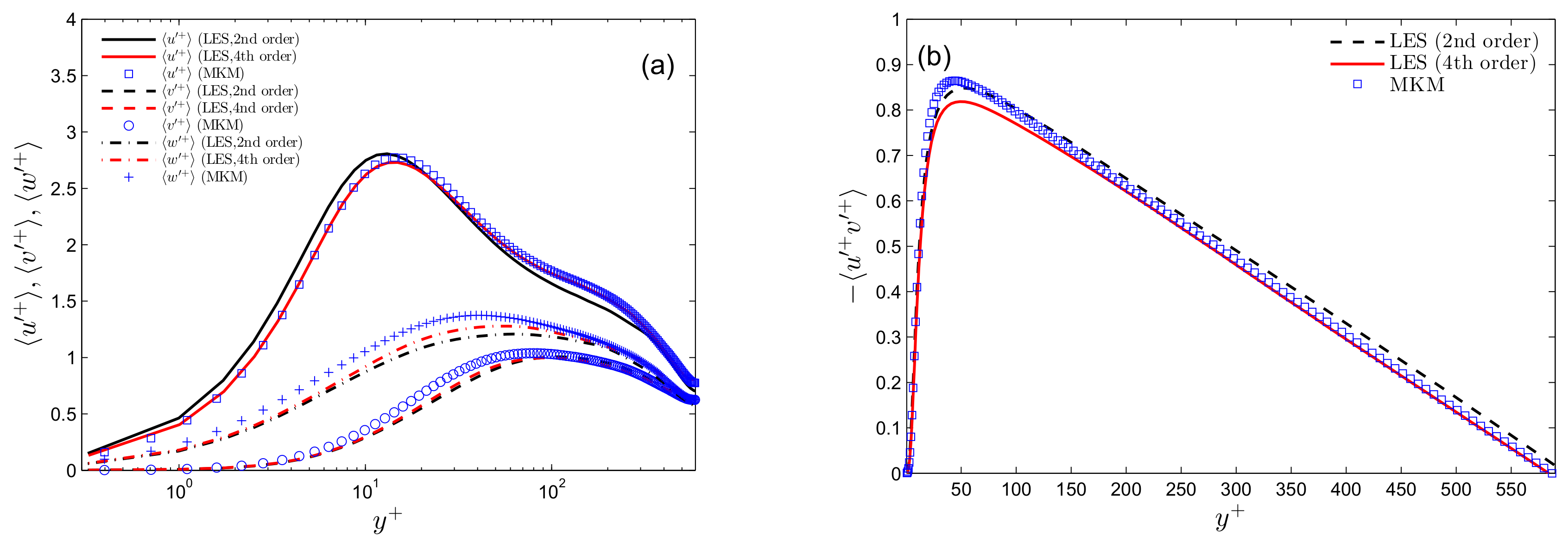
Figure 13.
One-dimensional streamwise pre-multiplied spectra at (a) and (b) of turbulent channel flow by LES at .
Figure 13.
One-dimensional streamwise pre-multiplied spectra at (a) and (b) of turbulent channel flow by LES at .
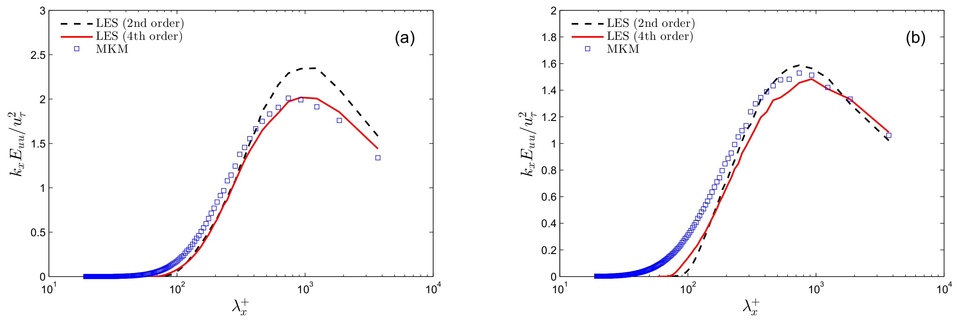
Figure 14.
Mean streamwise velocity of turbulent channel flow by WMLES at .
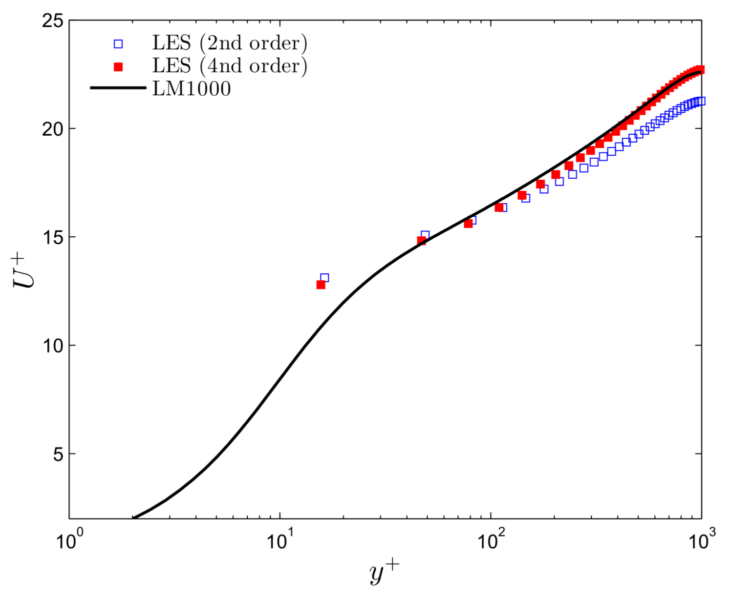
Figure 15.
(a) Normal and (b) shear Reynolds stresses of turbulent channel flow by WMLES at .

Figure 16.
(a) Streamwise and (b) spanwise premultiplied spectrograms of streamwise velocity and of turbulent channel flow at . The black lines indicate spectrogram isolines of LM1000 by DNS, the red lines by the second-order central difference WMLES, and the green lines by the fourth-order compact difference WMLES. The contour line levels are 0.1, 0.2, 0.4, 0.6, 0.8, 1.0, 1.5 and 2.0.

© 2018 by the authors. Licensee MDPI, Basel, Switzerland. This article is an open access article distributed under the terms and conditions of the Creative Commons Attribution (CC BY) license (http://creativecommons.org/licenses/by/4.0/).
Share and Cite
MDPI and ACS Style
Hu, R.; Wang, L.; Wang, P.; Wang, Y.; Zheng, X. Application of High-Order Compact Difference Scheme in the Computation of Incompressible Wall-Bounded Turbulent Flows. Computation 2018, 6, 31. https://doi.org/10.3390/computation6020031
AMA Style
Hu R, Wang L, Wang P, Wang Y, Zheng X. Application of High-Order Compact Difference Scheme in the Computation of Incompressible Wall-Bounded Turbulent Flows. Computation. 2018; 6(2):31. https://doi.org/10.3390/computation6020031
Chicago/Turabian StyleHu, Ruifeng, Limin Wang, Ping Wang, Yan Wang, and Xiaojing Zheng. 2018. "Application of High-Order Compact Difference Scheme in the Computation of Incompressible Wall-Bounded Turbulent Flows" Computation 6, no. 2: 31. https://doi.org/10.3390/computation6020031
Note that from the first issue of 2016, this journal uses article numbers instead of page numbers. See further details here.