Wind Pressure Distributions on Buildings Using the Coherent Structure Smagorinsky Model for LES

1
Institute of Technology, Shimizu Corporation, Tokyo 1358530, Japan
2
Numerical Flow Designing Co., Ltd., Tokyo 1410022, Japan
3
School of Civil Engineering, Chongqing University, Chongqing 400045, China
*
Author to whom correspondence should be addressed.
Computation 2018, 6(2), 32; https://doi.org/10.3390/computation6020032
Submission received: 22 January 2018
/
Revised: 4 April 2018
/
Accepted: 10 April 2018
/
Published: 14 April 2018
(This article belongs to the Special Issue Computational Methods in Wind Engineering)
Abstract
:A subgrid-scale model based on coherent structures, called the Coherent Structure Smagorinsky Model (CSM), has been applied to a large eddy simulation to assess its performance in the prediction of wind pressure distributions on buildings. The study cases were carried out for the assessment of an isolated rectangular high-rise building and a building with a setback (both in a uniform flow) and an actual high-rise building in an urban city with turbulent boundary layer flow. For the isolated rectangular high-rise building in uniform flow, the CSM showed good agreement with both the traditional Smagorinsky Model (SM) and the experiments (values within 20%). For the building with a setback as well as the actual high-rise building in an urban city, both of which have a distinctive wind pressure distribution with large negative pressure caused by the complicated flow due to the strong influence of neighboring buildings, the CSM effectively gives more accurate results with less variation than the SM in comparison with the experimental results (within 20%). The CSM also yielded consistent peak pressure coefficients for all wind directions, within 20% of experimental values in a relatively high-pressure region of the case study of the actual high-rise building in an urban city.
1. Introduction
Large eddy simulation (LES) generally shows good performance for the prediction of any turbulent flows. As is well known, LES solves large eddies on a grid scale (GS) and has been shown to implicitly account for small eddies using a subgrid-scale model (SGS model). The most-used SGS model is the Smagorinsky model (SM) [1]. The SM is determined using a model parameter. However, its model parameter must be changed to represent different turbulent flows such as a homogeneous isotropic turbulence, a turbulent mixing layer, or a turbulent channel flow.
Some SGS models have also been proposed to improve the weaknesses of the SM. A well-known SGS model is the dynamic Smagorinsky model (DSM) proposed by Germano et al. [2] that self-adjusts the model parameter using a dynamic approach. However, its parameter model often becomes negative and highly fluctuates in space and time, causing numerical instability.
To overcome this drawback, several models have been proposed. Ghosal et al. [3] proposed a dynamic localization model with the clipping operation. Meneveau et al. [4] proposed a Lagrangian averaging along the path line for the dynamic model. They are applicable to complex geometrical applications [5]; however, it still takes more computational time [4].
A number of local SGS models have been developed to offer several advantages over the SM. Yoshizawa et al. [6] suggested a nonequilibrium fixed-parameter SGS model and showed that the model was more accurate than the SM for turbulent channel flow. Vreman [7] suggested a localized filter SGS model and showed that it works better than the SM, as well as the DSM, for a turbulent mixing layer and turbulent channel flow. Park et al. [8] suggested a dynamic SGS model with a global coefficient model based on the global equilibrium between the SGS dissipation and the viscous dissipation, and showed that it works well for isotropic turbulence, turbulent channel flows, or the complex flow field over a circular cylinder or a sphere.
More recently, Kobayashi [9] proposed an SGS model based on coherent structures, called the Coherent Structure Smagorinsky model (CSM). Its model parameter is composed of a fixed model parameter and a coherent structure function, which is defined by the second invariant of the GS flow field normalized by the magnitude of a velocity gradient tensor, and it plays a role in wall-damping near the wall boundary. Some studies have indicated that the CSM produces better predictions than the DSM in a series of turbulent flow problems, such as turbulent channel flows [10], turbulent duct flows [11], or flows over complex geometries [12]. The CSM could run 15% faster in terms of the total CPU time than the DSM which gives it a significant advantage over the DSM [12]. In comparison with the SM, the model parameter that is used in the CSM does not need to change to model the different turbulent flows and is appropriate for large-scale computations [13].
For wind engineering problems, wind pressure is an important issue in building cladding design. Large negative wind pressures are commonly found on the roof and sidewall which are strongly related with the separation flow and vortex from the leading edges and corners of buildings [14,15,16]. The flow field is a distinctive and complex turbulent bluff body flow which differs from traditional turbulent flows such as turbulent channel flow. Some studies have indicated that LES could give sufficient accuracy for the prediction of the flow field around buildings, and of the wind load and wind pressure of isolated buildings or buildings in urban areas. However, it needs large-scale computation [17,18,19,20,21,22]. Several benchmark tests were done by the Architectural Institute of Japan [23] using LES with different Computational Fluid Dynamics (CFD) codes for an isolated high-rise building and for a complicatedly shaped building in an actual urban area with limited wind direction. It was indicated that LES could estimate the wind pressure with consistent accuracy within 20% in comparison with the target experimental results in these wind engineering problems [21,22,23]. However, most of these works used the SM model and did not provide an in-depth discussion of the SGS model details.
All SGS models are attractive for wind engineering problems. Among them is the CSM determined by the second invariant of the flow field which reflects the vortex structures. This makes it acceptable for strong vortex interference in the turbulent bluff body flow as well as for the building wind pressure problem. It is for this reason that we chose the CSM in the first stage. The other models remain to be explored in future study.
In this study, the applicability of the CSM is mainly assessed in the LES of wind pressure distributions acting on buildings. Two case studies are examined: isolated buildings in uniform flow and an actual high-rise building in an urban city with turbulent boundary layer flow. First, this paper briefly describes the SGS models. For each case study, the wind tunnel experiments and the target buildings are presented. Then, the numerical models and results are given and a discussion is presented on the performance of the CSM in comparison with the SM and experimental results.
2. SGS Models and Numerical Methods
2.1. SGS Models
In LES, the momentum equation is filtered with the grid filtering operator (-) as follows:
where x, t, u, p, , and are the spatial coordinate, time, velocity vector, pressure, density, and kinematic viscosity, respectively. is the Kronecker delta, and and denote the SGS stress tensor and the traceless SGS stress tensor, respectively. The SM and CSM are examined in the present study.
In the SM [1], the traceless SGS stress tensor based on the eddy viscosity concept is defined by the following equation:
where is the model parameter, is the filter width, and is the velocity strain tensor. The Smagorinsky constant as is used hereafter. Because the model parameter is always positive, the simulation of the SM can be stably carried out. However, the SM has some flaws [9,10,11,12]. The Smagorinsky constant must be changed depending on the flow field; for example, for homogeneous turbulences and for turbulent channel flows. The wall damping function is also required to modify the eddy viscosity both at the wall and near the wall. The explicit van Driest wall damping function is the most commonly used function. Within this function, the wall coordinate commonly results in high computational cost for large-scale models with unstructured meshes.
In the CSM, the traceless SGS stress tensor is determined by Equation (4). However, the model parameter is locally determined based on the coherent structure as follows [9]:
with
where CCSM is a fixed model constant, FCS is the coherent structure function defined as the second invariant Q normalized by the magnitude of a velocity gradient tensor E in a GS flow field, and FΩ is the energy decay suppression function. is the vorticity tensor in a GS flow field. The wall damping effect is introduced by the coherent structure function FCS, which reflects the behavior of the second invariant Q [9].
Moreover, FCS and FΩ have definite upper and lower limits [12]. Therefore, the CSM has small variance in the model parameter and the simulations performed using the CSM are more stable than the simulations that use other SGS models.
In addition, it should be noted that the second invariant Q is a useful parameter usually used to visualize the vortex structures in a wind flow field. Hence, the CSM has a quality that effectively assimilates the distinctive vortex structures separately from the buildings that cause the dominant wind pressures acting on the building surfaces.
2.2. Numerical Methods
In the present study, we used the pisoFoam solver from the open-source software OpenFOAM-2.0.0 [24] to solve the filtered governing equations for the LES. The discretization of the solver is based on the finite volume method of a cell-centered unstructured mesh.
For the numerical schemes, the linear scheme was used as a default to calculate the interpolation of values typically from cell centers to face centers (specified by “interpolationSchemes {default linear;}” in OpenFOAM). An implicit second-order backward scheme was used for the time derivative term (specified as “ddtSchemes {backward;}”). A second-order central difference scheme was used for the convective term (specified as “divSchemes {Gauss linear;}”). A Gaussian integration with linear interpolation was used for the gradient terms (specified as the default by “gradSchemes {Gauss linear;}”). A Gaussian integration, in which the surface normal gradient was specified by a limiter for the nonorthogonal correction, was used for the diffusion term (specified as “laplacianSchemes {Gauss linear limited 0.333;}”). Although assessing the numerical schemes for the accuracy of the simulation is attractive, the numerical dissipation from the second-order central difference scheme for the convective term [25] is also a valuable topic, but it is to be explored in further studies.
The momentum equation for velocity and the Poisson equation for pressure were solved using the linear equation solvers of the Biconjugate Gradient (BiCG) method and the Algebraic Multigrid (AMG) method, respectively. The Pressure-Implicit with Splitting of Operators (PISO) method was adopted for the pressure–velocity coupling of the transient flow calculations. A nonorthogonality correction was also used to modify the accuracy and stability of the diffusion term on the nonorthogonal meshes.
For the SGS models of LES, we used the SM in OpenFOAM with the default parameter in which the estimated Smagorinsky constant Cs was 0.13, and the explicit wall damping function was of the van Driest type. The CSM was developed as new code based on Equation (5) and the SM implementation code.
Furthermore, we used the wall-resolved LES (without using any wall layer models). The wall boundaries of the computational domains were set as no-slip boundaries. The finest grid size was small enough to have two grids within the viscous sublayer (more details in Phuc et al. [26]). However, target buildings in this study had rectangular shapes with sharp edges. For the cases of the building shapes, the separation points are generally fixed at the sharp edges and corners. Practically, there is not much Reynolds number dependence, and it is not critical for predicting the flow in the separation area of these buildings in comparison with others—for example, a circular cylinder or an airfoil.
3. Numerical Simulation for Isolated Buildings in Uniform Flow
3.1. Experiments for Validation
Two types of experiments—wind pressure experiments and particle image velocimetry (PIV) experiments in a uniform flow—were carried out to measure the wind pressure distribution on the building models and the flow fields around them. The experiments were done in a 104 m long wind tunnel at the Shimizu Corporation, Tokyo, Japan. The measurement section is 3.5 m wide and 2.5 m in height. Figure 1 shows pictures of the experimental setups. The building models were set up on a flat plate (width: 1 m; length: 1.8 m), which acted as a virtual foundation with a leading edge that was processed into a streamlined shape. The wind profile on the flat plate was examined using a hot-wire anemometer. It had a uniform flow with a wind speed of U0 = 10 m/s, and its turbulence intensity was less than 0.2%.
There were two target buildings: an isolated high-rise rectangular building called R01 (B/D/H = 2:1:2) with a height of 50 m, and a building with a setback, referred to as SBL. Herein, the building SBL constituted of a high-rise part based on the building R01, and a low-rise part which was packed closely featuring a building setback. The test models of the buildings were made of acrylic plastic at the scale of 1:250. Table 1 and Figure 2 describe the geometries of the building models. Experiments were conducted with a wind direction normal to the building. The Reynolds number (Re = U0B/ν, B = 0.2 m) was about 112,000.
For the pressure experiments, 412 pressure taps were concentrated at one side of the roofs and the walls (roof surfaces: R1 and R2; wall surfaces: W1 and W2) to measure the external wind pressure acting on the models. It was adequate to measure only one side due to their structural symmetries as shown in Figure 2. Experimental data were recorded for 8 s at a sampling frequency of 1000 Hz, and the variation of both the mean and peak pressures during the recorded time was less than 5%. The wind pressures of the roof and wall surfaces were statistically summarized: the peak pressure coefficients were estimated using a moving average with a window of one second of real time.
For the PIV experiments, the system consisted of a high-speed digital video camera (Plantom V7, maximum frame rate: 4800 frames/s, effective pixels: 800 × 600, sensor type: SR-CMOS), a double-pulse Nd:YAG laser (Lee Laser Inc., Orlando, FL, USA, average power 50 W, the power of the laser pulse is 19 mJ), a laser pulse synchronizer, and a tracer particle generator (PivPar40, oil mist with particle diameter: 1 μm). The tracer particles were discharged downstream of the building model and circulated inside the wind tunnel to create a uniform particle distribution. In order to manage the experimental conditions to be consistent with the pressure experiments, the laser sheet was precisely adjusted with high-intensity power. The video camera recorded for 3 s at a frame rate of 4000 frames/s due to PIV system limitations. The 4000 images taken each second were grouped into 2000 consecutive pairs, and each pair was used to calculate the flow field information. Figure 3 shows the planes that were chosen for the PIV experiments. The regions A1, A2, and A3 were used to examine the flow field at the central cross section of the models. The region B1 was 5 mm away from the wall surface W1 in order to examine the flow field near its corner.
3.2. Computational Model and Calculation Conditions
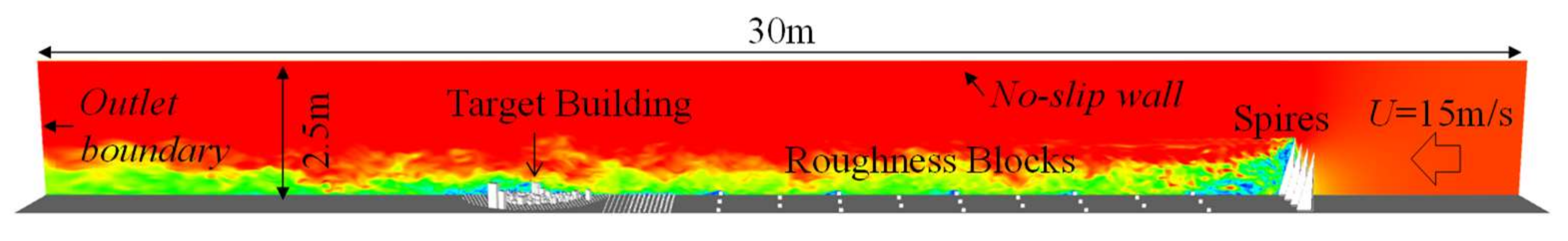
Figure 4 shows the computational domain which was 3 m wide, 6 m long, and 2.5 m high, including the flat plate and building model. The inflow condition was set as a uniform flow of U0 = 10 m/s. The outlet boundary was an open boundary with an inletOutlet condition [24]. The walls of the building model and the flat plate were no-slip boundaries. The other boundaries were slip boundaries.
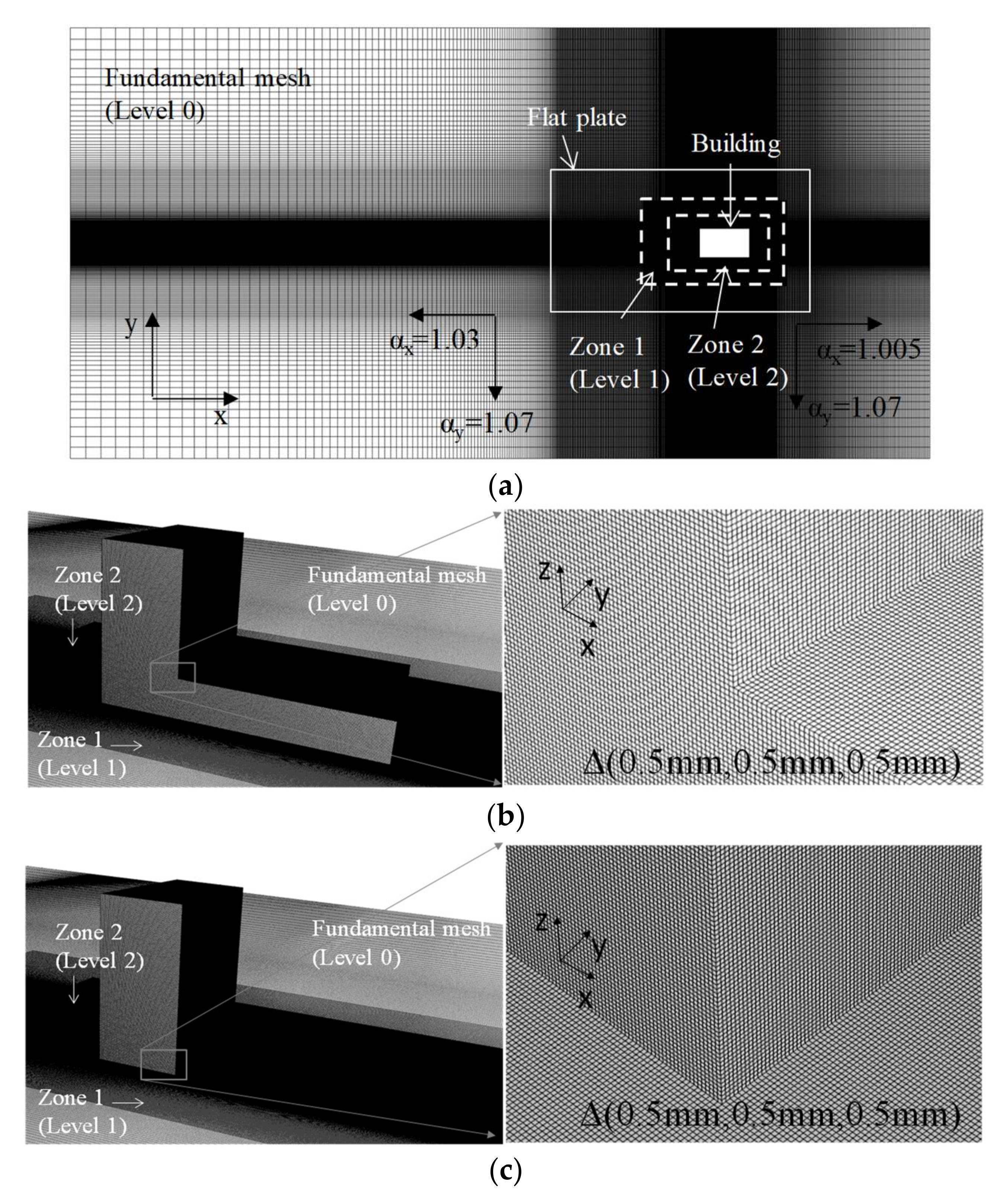
Meshes were generated using the snappyHexMesh system from OpenFOAM [24]. Figure 5 depicts the entire mesh in the plane view, the surface meshes of the building model R01 and SBL in the vicinity, and a close-up of their corners. A fundamental mesh was constructed with a mesh size of 2 mm near the building model, then stretched out with factors of 1.005 in the upstream and 1.03 in the downstream x directions, 1.07 in the y direction, and 1.07 in the z direction. Then, the mesh cells were refined for two further levels to achieve a high resolution around the building model in which the nearest mesh size Δ was 0.5 mm. The total mesh cells for each model numbered about 570 million.
Table 2 describes the calculation conditions. LESs with the SM and the CSM were carried out. The results obtained from these SGS models were verified by comparison with experimental results, mainly to clarify the performance of the CSM. Time steps Δt were 1 × 10⁻⁴, 5 × 10⁻⁵, and 2.5 × 10⁻⁵ (s), corresponding to the approximated Courant numbers () of 2.0, 1.0, and 0.5, respectively. The simulations were conducted using the 6144 parallel CPUs in “The K Computer”, which was the world’s first-ranked supercomputer of the TOP500 Supercomputers in 2012. Peak pressure coefficients of the building models were calculated from the results of a real-time 1.0 s moving average—the same as the average calculated in the experiment.
3.3. Results and Discussion
3.3.1. Pressure Coefficients of Buildings
This section discusses the mean and negative peak pressure coefficients, which are important parameters for the assessment of building cladding design. Here, the wind pressure coefficient Cp is calculated as follows:
where p0 and UH are the reference pressure at a 1.4 m height above the building and the wind speed at the eave height of the building, respectively. In this case, the inflow condition was set as the uniform flow, so the wind speed UH is equal to U0 = 10 m/s.
Figure 6 shows the distributions of these coefficients for the buildings R01 and SBL in uniform flow. In comparison with the building R01, the building SBL has a specific pressure distribution on the sidewall surface with an unexpectedly large mean pressure coefficient of −1.3 and a negative peak pressure coefficient of −3.0 at its corner.
Figure 7 shows the mean and negative peak pressure coefficients obtained from LES using the SM and the CSM for the buildings R01 and SBL in comparison with the experimental results. For the building R01, the pressure coefficients of the SM and CSM are very similar and consistent with the experimental results (values within 20%). For the building SBL with a specific pressure distribution and large pressure coefficients, the SM results show quite a large difference from the experimental data in both positive and negative wind pressure regions. However, the CSM shows good agreement with the experimental results (within 20%).
Figure 8 shows the mean and negative peak pressure coefficients obtained from both the experiments and LES using the CSM with a Courant number, Cr, of 2.0, 1.0, or 0.5, respectively, for the buildings R01 and SBL. The pressure coefficients calculated using the CSM are consistent with the experimental results for both buildings. Decreasing the Cr caused the simulated mean and negative peak pressure coefficients to more closely match the experimental results. In particular, the mean pressure coefficient of −1 or less, and negative peak values of −2 or less, agreed well with the experimental values.
3.3.2. Flow Fields around Buildings
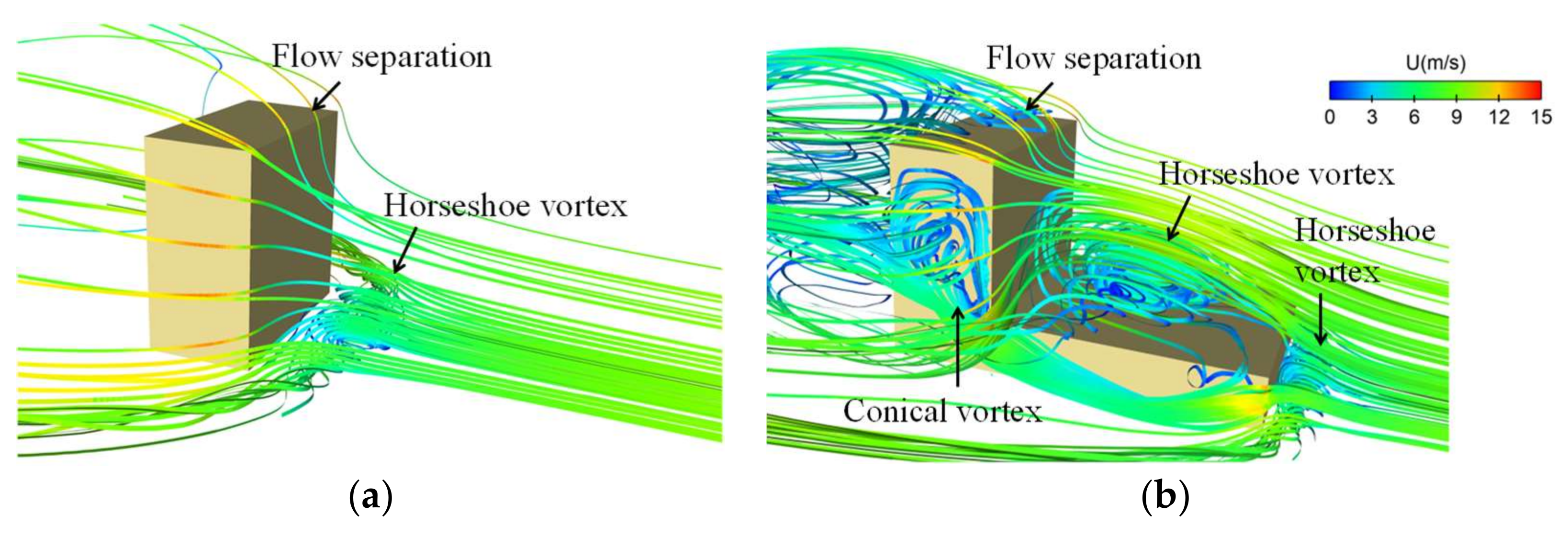
In order to understand the characteristics of the flow field around the buildings, the PIV results are considered. Figure 9a,b show the mean velocity vector and average vorticity contour in the planes A1, A2, and A3 of the central cross section of the buildings R01 and SBL as obtained by the PIV experiments. Figure 9c,d show these results in the plane 5 mm away from the sidewall surface near the corner where the unexpected, large negative peak coefficient occurred, as shown in Figure 6c,d. A three-dimensional visualization was also done to clarify the flow field structure around the buildings. The mean streamline estimated from the results of the CSM is shown in Figure 10.
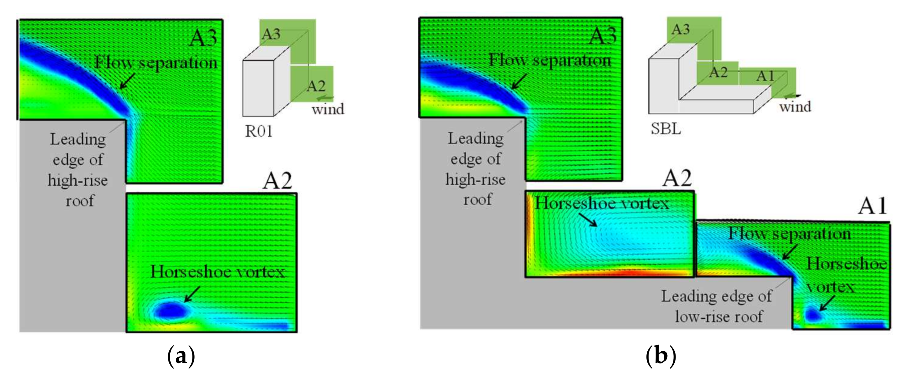
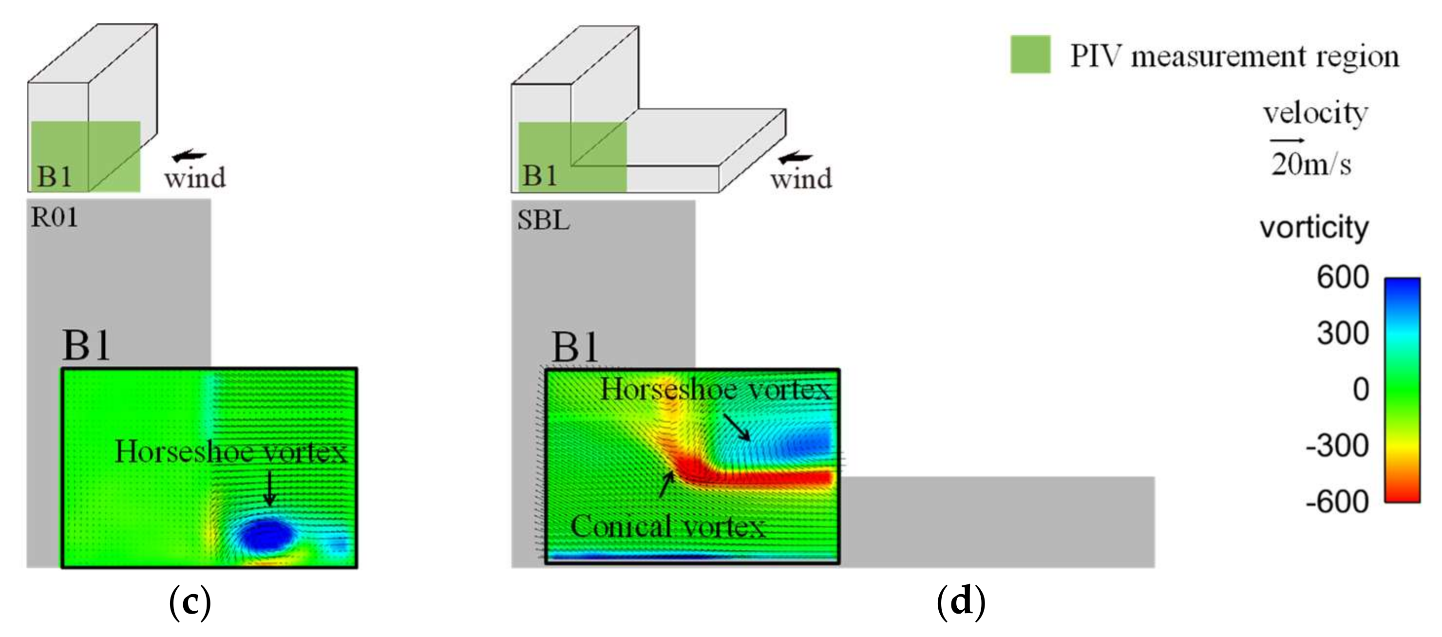
For the building R01 (Figure 9a and Figure 10a), a well-known horseshoe vortex is found in the vicinity of the lower part of the front of the building. A strong flow separation is generated from the leading edge of the roof surface, and they seem to behave independently. In the building SBL (Figure 9b and Figure 10b), two vortices formed in front of the lower and upper parts of the building. The former vortex is a horseshoe vortex. The latter vortex is generated by the complex interaction of the flow field separated from the leading edge of the lower roof, and the downward flow at the windward wall of the upper part of the building. As a result, this vortex becomes larger than the other ones. In addition, the flow separation at the upper part of the leading edge of the roof (Figure 9b) is slightly weaker than the flow separation from the building R01 (Figure 9a). In the plane 5 mm from the sidewall (Figure 9d), an upward flow with strong vorticity is also found near the corner of the sidewall W1 that generated a distinctively complex flow. Furthermore, these vortices and the flow separations of the building SBL (Figure 10b) seemingly interfere with each other more than do those from building R01 (Figure 10a).
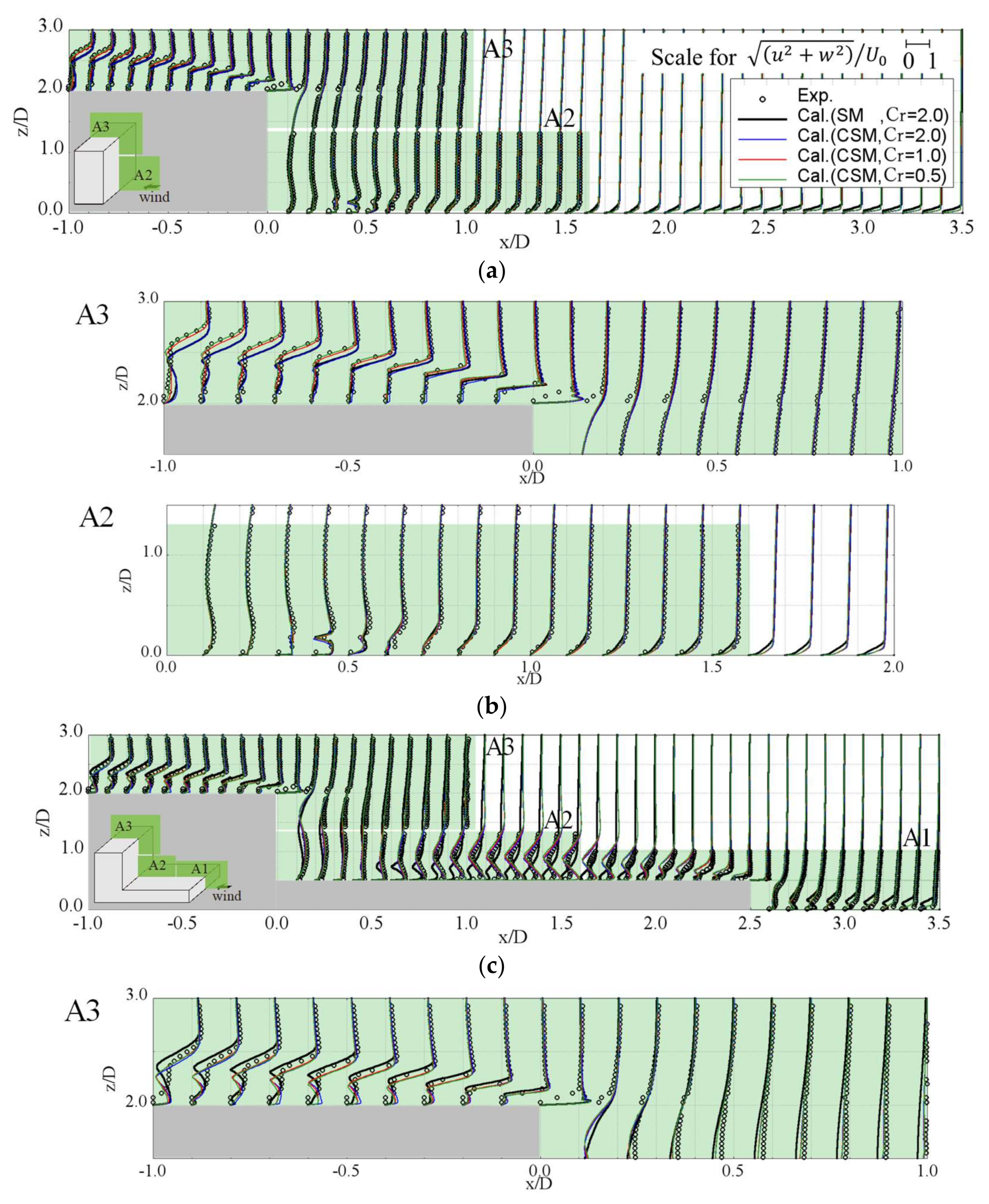
Figure 11 shows the profiles of the mean velocities and partial enlarged views calculated using the SM and CSM (Cr = 2.0) in comparison with the PIV results across the planes A1, A2, and A3 in both buildings R01 and SBL. For building R01, as shown in Figure 11a,b, a boundary layer is developed on the flat plate in the region x/D = 1.0–3.5. The behavior of the horseshoe vortex in the lower part of the front of the building is in the region x/D = 0–1.0. The region after x/D = 0 corresponds to the flow separation at the leading edge of the roof. The overall profiles calculated using the SM and the CSM are almost the same in these regions. For the building SBL, the region of x/D = 0.0–3.5 (Figure 11c,d) is the interference region of the vortices and the flow separation. The SM under-predicts this region, but the CSM shows good agreement with the PIV experiments. In particular, the CSM gives a profile with a level of accuracy similar to the PIV results in the region of the large vortex. As discussed in Section 2, the model parameter of the CSM is defined by the second invariant Q which is a quantity to describe the vortex structures. It appears that the CSM might reflect the vortex behaviors and simulate well the interference between the vortex and the flow separation in the complex flow field. Even at high computational model resolutions, the SGS model could affect the results of the velocity profiles.
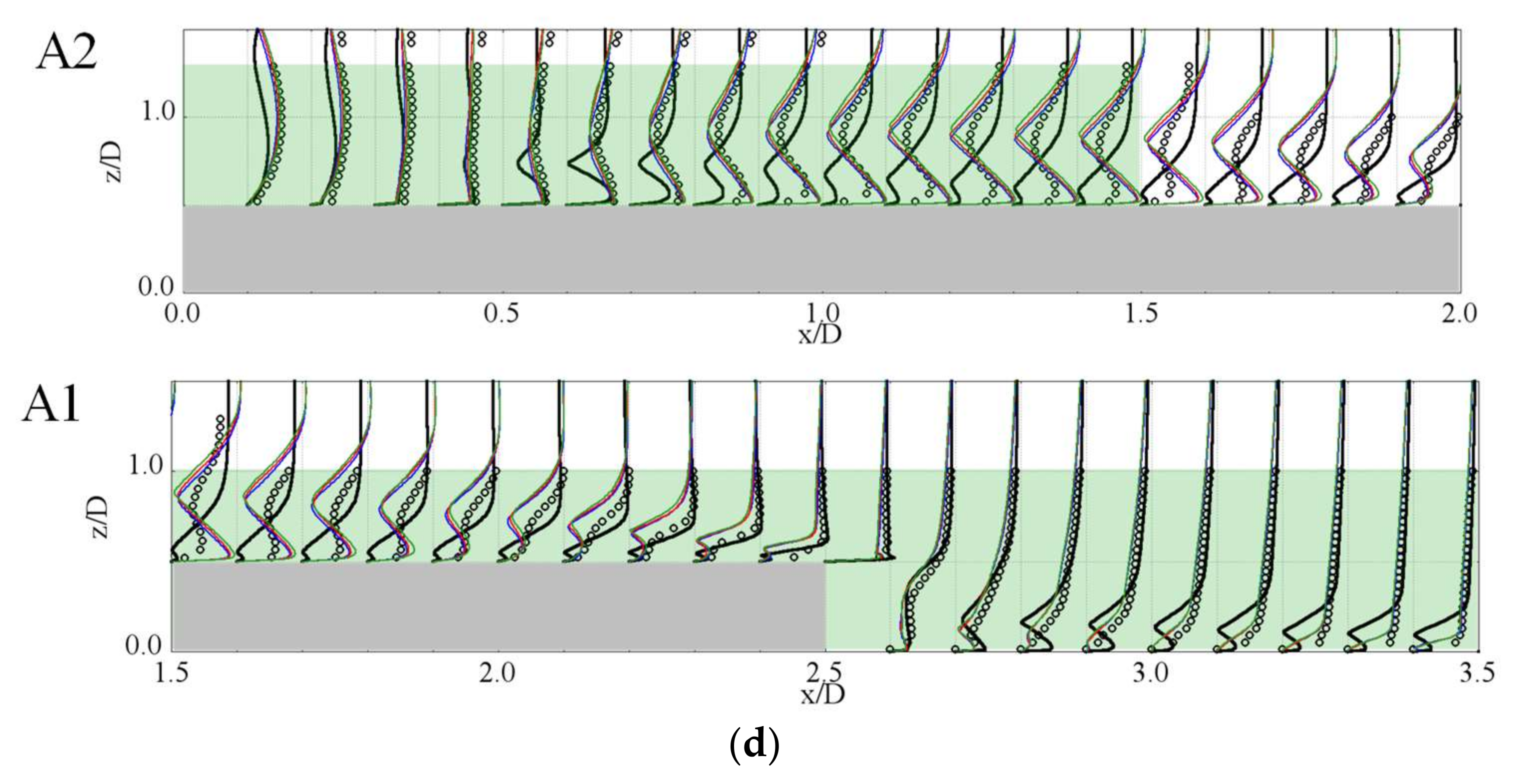
Figure 12 shows the profiles and partially enlarged views of mean velocities in the plane 5 mm away from the sidewall of these buildings. Again, the SM and CSM are in good agreement with the PIV results for the building R01 (Figure 12a,b). For the building SBL, the SM results are under-predicted, but the CSM predictions more closely match the results of the PIV experiments in the region of x/D = −1 to 1 as shown in Figure 12c,d.
4. Numerical Simulation for a High-Rise Building in an Urban City with Turbulent Flow
4.1. Validation Experiments
In this section, an actual high-rise building with a height of 100 m (D/B/H = 1:2:3) with uneven surfaces is investigated. Herein, the building is constructed in a dense urban area in which medium-rise buildings are packed closely together. The pressure experiment was carried out at a scale of 1:400. Figure 13 shows the experimental setup and the test model inside the 104 m long circuit boundary layer wind tunnel at the Shimizu Corporation, Tokyo, Japan. The test section is 3.5 m wide and 2.5 m high.
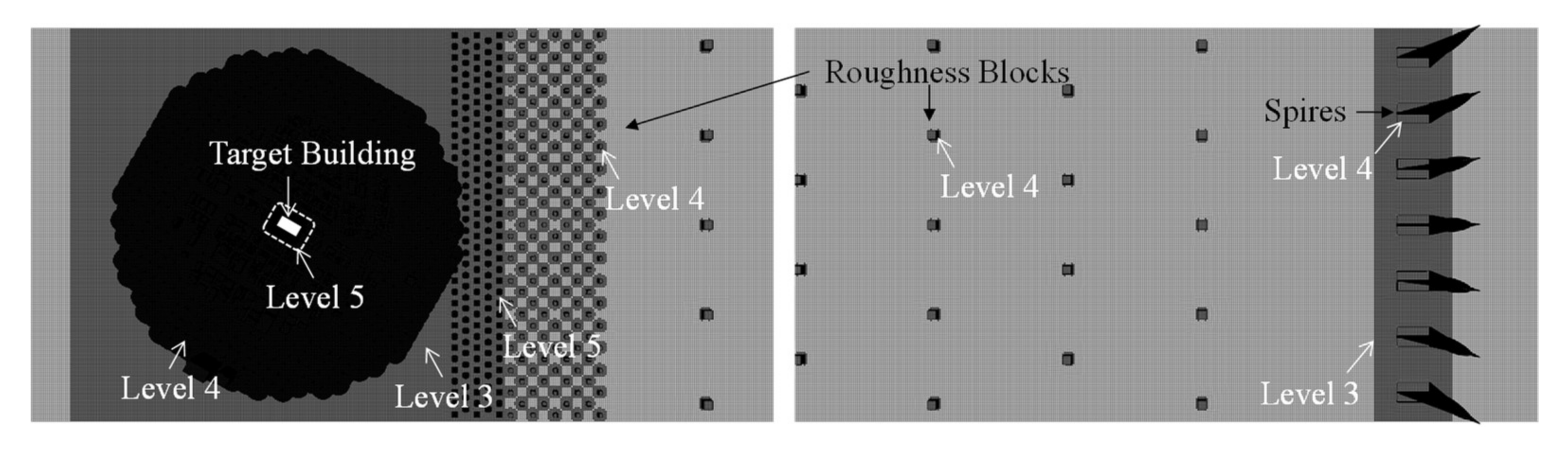
The approaching flow field was generated using spires and roughness blocks to satisfy the flat suburban terrain with few medium-rise buildings, of Category III according to the Architectural Institute of Japan [27]. During the experiment, the wind tunnel fan’s rotation was constantly controlled to maintain an approximate mean wind speed, UH, of 11 m/s at the test model eaves height (H = 0.25 m), which corresponds to a basic wind speed of 36 m/s in terms of real-time conversion. The vertical wind profile at the center of the turntable was measured using a hot-wire anemometer. The mean wind profile was examined using a power law of exponent, α, of 0.2 and longitudinal wind turbulence intensity, Iu, of 15% at the eaves height, H, of the building. The Reynolds number (Re = UHD/ν, D = 0.085 m) of the experiment was about 52,000.
Data logging equipment was used to measure the external pressures acting on the target building at 234 different points on the wall surfaces, arranged in 9 layers at different heights. The measurements were carried out for 36 wind directions at 10 degree intervals. Experimental data were recorded for about 30 s at a sampling rate of 1000 Hz, corresponding to five data samples in each ten-minute record in terms of real-time conversion (one sample for each ten-minute record is 6 s in experimental time). The external wind pressures measured on the wall surfaces were used to estimate the mean, standard deviation, and largest positive and negative peak pressure coefficients of the target building. The peak pressure coefficients, which are required for building wall cladding assessment, were moving-averaged using five samples, corresponding to a real-time moving average window of 0.5 s. The results for the 60 degree wind direction are discussed in detail in this paper due to the strong influence of neighboring buildings on this wind direction.
4.2. Computational Models and Calculation Conditions
A 30 m long computational domain was constructed to conscientiously model the wind tunnel measurement section including spires, block roughness, and buildings as shown in Figure 14. Two meshes with different resolutions (Meshes A and B) were generated using the snappyHexMesh system [24]. Figure 15 and Figure 16 show the surface mesh of the spire and roughness blocks, the building model in the vicinity, and an enlarged view of the top corner for a wind direction of 60 degree. The fundamental meshes of the snappyHexMesh system (Level 0) were generated at a mesh size with dimensions 64 mm × 64 mm × 32 mm for Mesh A, and 32 mm × 32 mm × 16 mm for Mesh B. Then, the mesh cells around the target building were refined to achieve a high resolution (Level 7) in which the smallest mesh cell size was 0.5 mm for Mesh A, and 0.25 mm for Mesh B. The total numbers of cells in Meshes A and B were about 140 million and 1.1 billion, respectively.
The boundary conditions are shown in Figure 14. The inflow condition is a uniform velocity U = 15 m/s in order to obtain a wind velocity at the eaves height, UH, of 11 m/s—the same as in the wind tunnel experiment. The outlet boundary is an open boundary with an inletOutlet condition [24]. The walls of the building model and wind tunnel are no-slip boundaries.
Table 3 describes the calculation conditions. Firstly, LES was performed with two SGS models: the SM and the CSM were carried out for Meshes A and B for a wind direction of 60 degree. The results obtained from these SGS models were verified by comparison with the experimental results. Next, the simulations for all wind directions (36 wind directions at 10 degree intervals) were conducted for one sample corresponding to a ten-minute record when converted to real time. Statistical data such as the largest peak pressure coefficients for all wind directions were evaluated. Hence, the peak pressure coefficients were estimated from the samples of a real-time 0.5 s moving average, as was the case in the experiment. By using OpenFOAM, a simulation of 6 s (corresponding to one sample in each ten-minute record when converted to real time) with Mesh A for each wind direction took about 20 days for the CSM and 40 days for the SM in terms of computational time using 768 parallel CPUs of “The K Computer”. It was found that the calculation of the wall coordinate y+ for the SM in OpenFOAM using the wave propagation method resulted in a significantly higher computational cost due to the complex geometry of the unstructured mesh and the large-scale computational domain of several hundred million mesh cells.
4.3. Results and Discussion
4.3.1. Wind Flow Characteristics
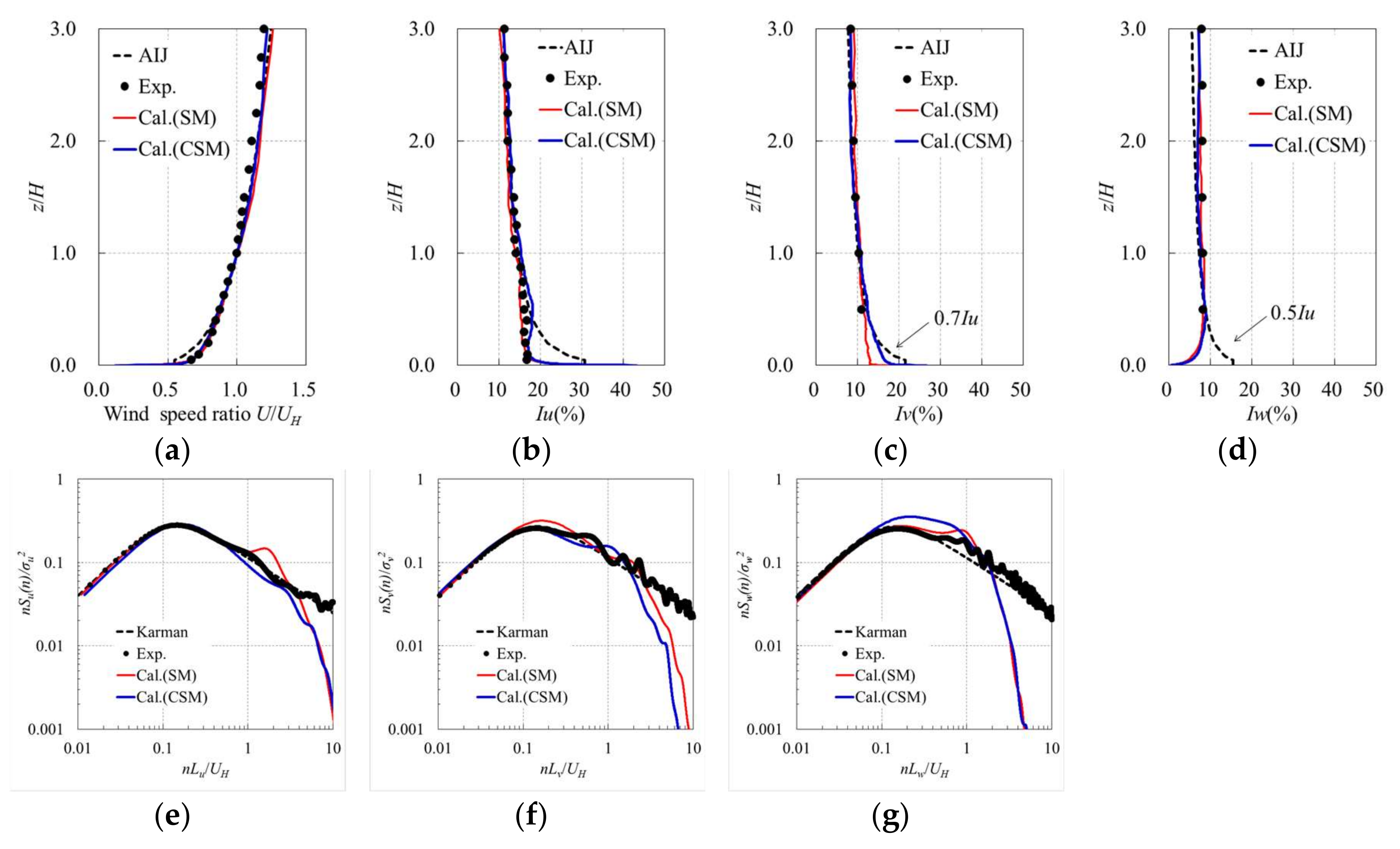
Figure 17 illustrates the vertical profiles of the mean wind speed, turbulence intensity, and power spectrum densities of the three wind components (longitudinal component u, lateral component v, and vertical component w) as obtained at the center of the turntable for the case of Mesh A without buildings. Because of the precise modeling of the wind tunnel measurement section, the mean wind profile and turbulence intensities calculated using both the SM and the CSM show very good agreement with the experimental values and also agree with the profiles of the Architectural Institute of Japan [27]. The experimental and calculated power spectral densities are compared with the Karman spectrum. Although the experimental power spectrum densities of the wind components are consistent with the Karman spectrum, the calculated results are significantly lower in the high-frequency region, where the normalized frequencies are less than 2 on account of the fineness of the computational mesh.
4.3.2. Flow Fields around the Target Building
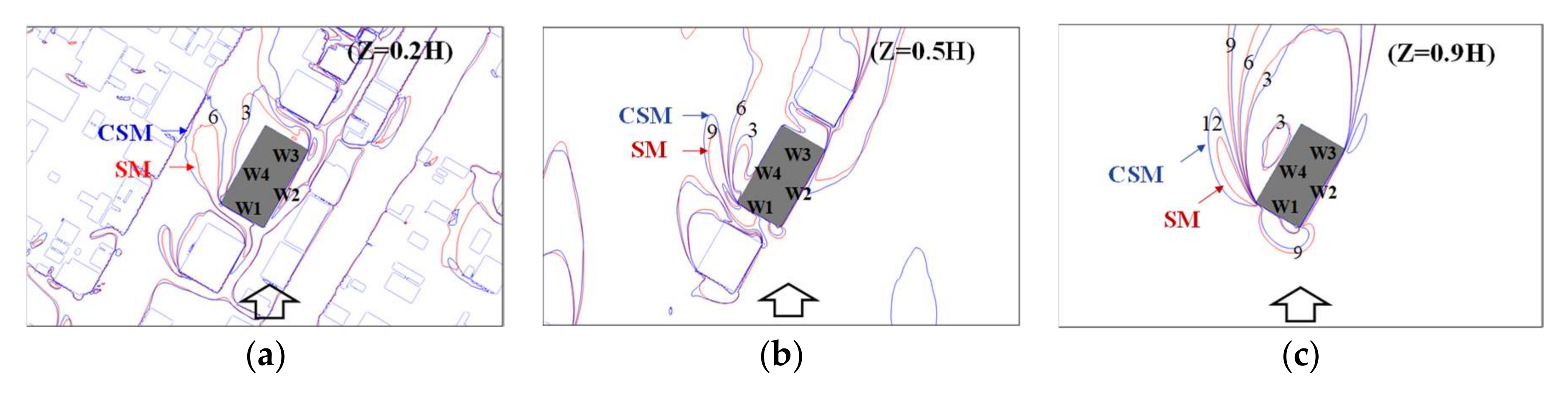
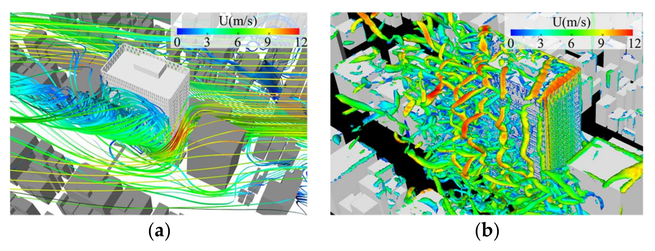
In order to understand the flow fields around the target building, the contours of the mean wind speed around the target building at heights z = 0.2H, 0.5H, and 0.9H for the 60 degree wind direction, as obtained from LES using the SM and the CSM with Mesh A, are shown in Figure 18. Moreover, Figure 19 shows the mean streamline and instantaneous Q-criterion isosurface (Q = 300,000) obtained from the three-dimensional visualization. The flow field around the target building is greatly deformed in the vertical direction. At height z = 0.2H, the flow field substantially follows the street due to the influence of the densely packed surrounding buildings. However, the influences of the upstream and downstream adjacent medium-rise buildings are remarkable at the height z = 0.5H. Separated shear layers generated from the target building and adjacent buildings are strongly coupled and greatly deformed. At height z = 0.9H, which exceeds the height of the adjacent medium-rise buildings, the flow field is the same as the typical flow field around an isolated building. As a result, a complex three-dimensional flow with strong vortices separated from the leading edges is formed due to the strong influence of the windward neighboring buildings.
We compared the results of the SM and CSM models as shown in Figure 18 and found a difference in the separated shear layers generated from the target building and its adjacent buildings. The CSM gives a larger flow separation than the SM in the situation. It seems that the SM underestimated the flow field in the separation area. Related to Figure 19, this separation area has a strong effect from the vortex separated from the leading edges. The CSM, whose model parameter is defined from the Q-criterion as a quantity for description of the vortex structure, takes into account the effect of the vortex behavior. Therefore, it may simulate the situation well.
4.3.3. Pressure Coefficients of the Target Building for a Specific Wind Direction
Figure 20 shows the mean pressure coefficients of the target building as estimated from the experiments. The figure also shows the coefficients estimated from one sample obtained using LES with the SM and the CSM with different meshes. A distinctive pressure distribution is found on the front wall, W1, in which a strong positive pressure coefficient occurs at the upper right portion, while a negative pressure coefficient occurs at the lower left portion. This can be understood from the flow field around the target building due to the strong influence of the adjacent buildings mentioned above. Generally, the CSM gives a better pressure distribution than does the SM in comparison with experimental data.
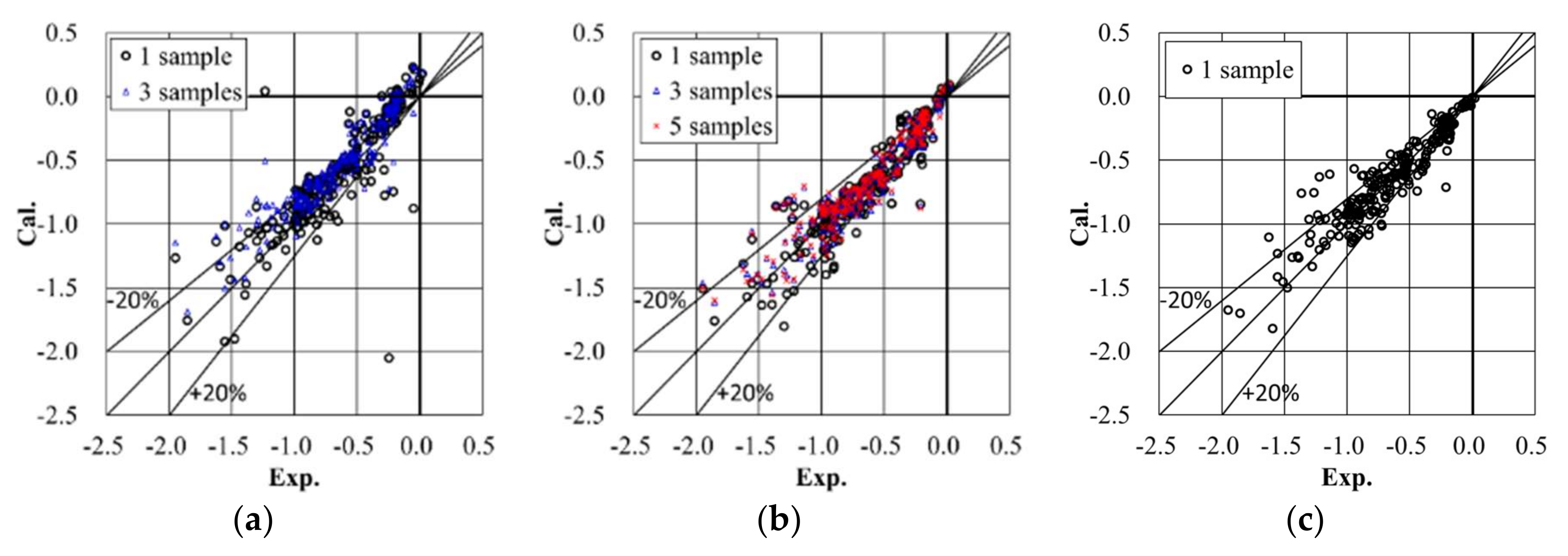
Figure 21 and Figure 22 show a comparison of the mean and largest negative peak pressure coefficients between the experimental results (values within 20%) and LES for the first sample, averaged from three samples or five samples. We found that the variation of the SM is large, and that the CSM gives more accurate results and less variation than does the SM. Using a finer mesh (Mesh B) yields better results, which are especially consistent with experimental results (discrepancy of less than 20%) in the relatively high-wind-pressure region that is important in building cladding assessments.
Moreover, it is interesting to compare the average results from all samples with the first sample’s results for the SM and CSM predictions. When using the SM as shown in Figure 21a and Figure 22a, it is evident that the variation of the first sample is more scattered than the variation in the value averaged from the three samples. When using the CSM, as shown in Figure 21b and Figure 22b, the variations averaged from three samples or five samples are quite similar to the variation of the first results. As a result, we suggest that the CSM is an effective method for understanding coherent structures within a flow field.
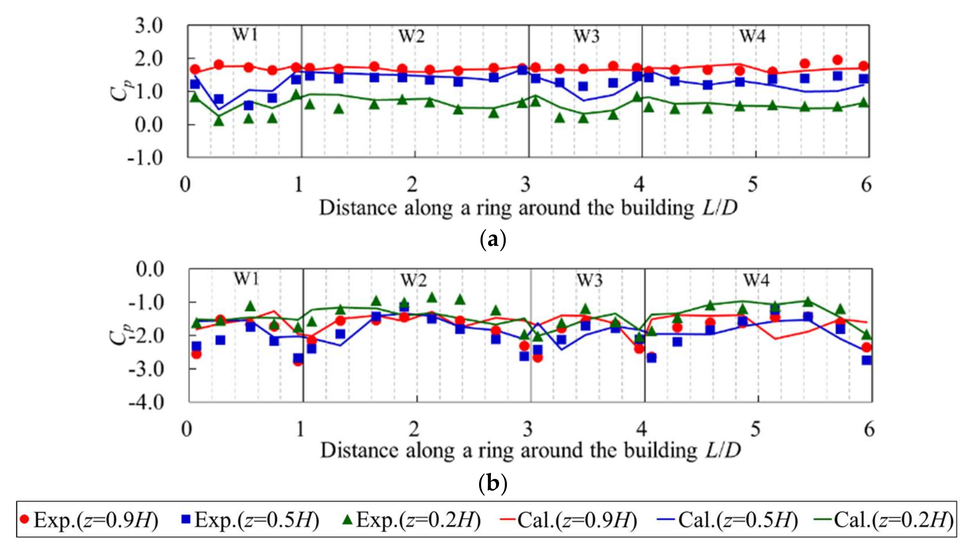
Figure 23 shows the mean, standard deviation, and largest positive and negative peaks of the pressure coefficients averaged from five samples, obtained from the experiments and LES using the CSM with Mesh A at heights z = 0.2H, 0.5H, and 0.9H. Whereas the coefficients of the walls W2 and W3 are almost the same, the values for wall W1 differ in the vertical direction. A large negative peak value is found on the medium-rise section (z = 0.5H) on wall W4. The simulation results show good agreement with the experimental results.
4.3.4. Pressure Coefficients of the Target Building for All Wind Directions
The previous section discussed the CSM results for a specific wind direction. Commonly, the wind pressure distributions on a building in an urban area change according to the wind direction and depend on the influence of different neighboring buildings. To assess the universality of the CSM for predicting wind pressure distributions on a building, similar mesh generations and simulations for all 36 wind directions at 10 degree intervals were conducted.
Figure 24 shows the largest positive and negative peak pressure coefficients estimated from all 36 wind directions, as estimated from the experiments and LES using the CSM (Mesh A) for the first sample. The calculated peak pressure coefficients are consistently within 20% of the experimental values in the relatively high-pressure region—the same as the results for the specific wind direction as shown in the previous section. Furthermore, the consistent accuracy of these results is found to be at least similar to or less than the wind tunnel coefficients of variation (COVs) as discussed by Tamura and Phuc [20] in their assessment of the variation in a series of wind tunnel test results.
In addition, Figure 25 shows these peak pressure coefficients at the heights z = 0.2H, 0.5H, and 0.9H. The numerical simulation results show quite a good agreement with the experimental results.
5. Conclusions
Case studies using LES have been carried out to investigate the performance of the CSM in predicting the wind pressure distributions on buildings in various flow fields. Comparison between the SM results and experimental results led to the following conclusions:
- For an isolated rectangular building in uniform flow, the flow field around the building is generated by the horseshoe vortex and separated flow. Both SM and CSM show good agreement with the PIV results in the flow separation region as well as in the horseshoe vortex regions. The wind pressure coefficients calculated using both SM and CSM consistently agree with the experimental results (values within 20%).
- For an isolated building with a setback in uniform flow, a complex flow field is generated by a distinctive large horseshoe vortex interfering with the separated flow from the lower roof. A large negative pressure coefficient is found at the corner of the sidewall, near the interfered-with area. Although using the SM results in under-prediction, the predictions made using the CSM show good agreement with the PIV results for the flow field. This means that the CSM with the model parameter based on the coherent structure reflects the vortex behaviors and simulates well the complex flow fields due to the strong interference of the vorticities and flow separations. The CSM results also showed much better performance than the SM results for the wind pressure distribution on this building, being within 20% of the experimental results.
- For a high-rise building in an actual urban city with a turbulent boundary layer flow, we found that a strong three-dimensional complex wind flow occurs due to the strong influence of neighboring buildings, including interference of vortices and separated flows. We also found a distinctive wind pressure distribution that had strong positive and negative pressures simultaneously occurring on the front wall of the target building. The CSM also gives more accurate results with less variation than the SM, being within 20% of experimental results. In addition, LES with the CSM was conducted for all wind directions. The calculated largest positive and negative peak pressure coefficients were consistently in good agreement with experimental results (within 20%) in the relatively high-pressure region, at least similar to or less than the COVs of the wind tunnel test results [20].
Furthermore, it should be mentioned again that LES solves large eddies/vortices on a grid scale (GS), and takes account of small eddies on a sub-grid scale (SGS) using an SGS model. The difference between the SM and the CSM is only a model parameter of an SGS model. This model parameter is determined by a Smagorinsky constant for the SM, but is specifically determined by a second invariant parameter for the CSM which could describe the effect of the vortex structures from the GS.
From the results of the case of an isolated rectangular building, it is found that the SGS models are not sensitive to the flow field around the building (including the horseshoe vortex and separated flow). The grid size is seemingly small enough for LES to resolve the flow field in the GS, or the effect from the small eddies in the SGS is not so dominant. From the results of the case of an isolated building with a setback as well as the case of a high-rise building in an actual urban city, the CSM showed better performance than the SM. This implies that the small eddies become more activated in the flow fields of the interference of the vortices and separated flows. The activation is found to be related to the vortex structures from the GS.
It could be useful to investigate the contribution of the CSM parameters to understand these flow fields, or to develop a much more appropriate SGS model. However, this remains for future studies.
Acknowledgments
This research used the computational resources of the K computer provided by the RIKEN Advanced Institute for Computational Science through the HPCI System Research project (Project ID: hp150031, hp160054).
Author Contributions
P.V.P. performed the experiments and simulations, analyzed the data and wrote the paper; T.N. and H.K. performed some experiments and discussions; K.H. and Y.T. participated in the discussions.
Conflicts of Interest
The authors declare no conflict of interest.
References
- Smagorinsky, J. General circulation experiments with the primitive equations I, The basic experiment. Mon. Weather Rev. 1963, 91, 99–164. [Google Scholar] [CrossRef]
- Germano, M.; Piomelli, U.; Moin, P.; Cabot, W.H. A dynamic subgrid-scale eddy viscosity model. Phys. Fluids 1991, 3, 1760–1765. [Google Scholar] [CrossRef]
- Ghosal, S.; Lund, T.S.; Moin, P.; Akselvoll, K. A dynamic localization model for large-eddy simulation of turbulent flows. J. Fluid Mech. 1995, 286, 229–255. [Google Scholar] [CrossRef]
- Meneveau, C.; Lund, T.S.; Cabot, W.H. A lagrangian dynamic subgrid-scale model of turbulence. J. Fluid Mech. 1996, 319, 353–385. [Google Scholar] [CrossRef]
- Murakami, S. Current status and future trends in computational wind engineering. J. Wind Eng. Ind. Aerodyn. 1997, 67–68, 3–34. [Google Scholar] [CrossRef]
- Yoshizawa, A.; Kobayashi, K.; Kobayashi, T.; Taniguchi, N. A nonequilibrium fixed-parameter subgrid-scale model obeying the near-wall asymptotic constraint. Phys. Fluids 2000, 12, 2338–2344. [Google Scholar] [CrossRef]
- Vreman, A.W. An eddy-viscosity subgrid-scale model for turbulent shear flow: Algebraic theory and applications. Phys. Fluids 2004, 16, 3670–3681. [Google Scholar] [CrossRef]
- Park, N.; Lee, S.; Lee, J.; Choi, H. A dynamic subgrid-scale eddy viscosity model with a global model coefficient. Phys. Fluids 2006, 18, 125109. [Google Scholar] [CrossRef]
- Kobayashi, H. The subgrid-scale models based on coherent structures for rotating homogeneous turbulence and turbulent channel flow. Phys. Fluids 2005, 17, 045104. [Google Scholar] [CrossRef]
- Kobayashi, H. Large eddy simulation of magnetohydrodynamic turbulent channel flows with local subgrid-scale model based on coherent structures. Phys. Fluids 2006, 18, 045107. [Google Scholar] [CrossRef]
- Kobayashi, H. Large eddy simulation of magnetohydrodynamic turbulent duct flows turbulent duct flows. Phys. Fluids 2008, 20, 015102. [Google Scholar] [CrossRef]
- Kobayashi, H.; Ham, F.; Wu, X. Application of a local SGS model based on coherent structures to complex geometries. Int. J. Heat Fluid Flow 2008, 29, 640–653. [Google Scholar] [CrossRef]
- Onodera, N.; Aoki, T.; Shimokawabe, T.; Kobayashi, H. Large-scale LES Wind Simulation using Lattice Boltzmann Method for a 10 km × 10 km Area in Metropolitan Tokyo. Tsubame ESJ 2013, 9, 2–8. [Google Scholar]
- Melbourne, W.H. Turbulence and the leading edge phenomenon. J. Wind Eng. Ind. Aerodyn. 1993, 49, 45–63. [Google Scholar] [CrossRef]
- Okuda, Y.; Taniike, Y. Conical vortices over side face of a three dimensional square prism. J. Wind Eng. Ind. Aerodyn. 1993, 50, 163–172. [Google Scholar] [CrossRef]
- Kawai, H. Local peak pressure and conical vortex on building. J. Wind Eng. Ind. Aerodyn. 2002, 90, 251–263. [Google Scholar] [CrossRef]
- Tominaga, Y.; Mochida, A.; Yoshie, R.; Kataoka, H.; Nozu, T.; Yoshikawa, M.; Shirasawa, T. AIJ guidelines for practical applications of CFD to pedestrian wind environment around buildings. J. Wind Eng. Ind. Aerodyn. 2008, 96, 1749–1761. [Google Scholar] [CrossRef]
- Tamura, T.; Miyagi, T.; Kitagishi, T. Numerical prediction of unsteady pressures on a square cylinder with various corner shapes. J. Wind Eng. Ind. Aerodyn. 1998, 74–76, 531–542. [Google Scholar] [CrossRef]
- Tamura, T.; Nozawa, K.; Kondo, K. AIJ guide for numerical prediction of wind loads on buildings. J. Wind Eng. Ind. Aerodyn. 2008, 96, 1974–1984. [Google Scholar] [CrossRef]
- Tamura, Y.; Phuc, P.V. Development of CFD and applications: Monologue by a non-CFD-expert. J. Wind Eng. Ind. Aerodyn. 2015, 144, 3–13. [Google Scholar] [CrossRef]
- Yoshikawa, M. Wind load for cladding. In Material of Panel Discussion of Steering Committee for Loads on Buildings at Annual Meeting of AIJ in Tokai; Architectural Institute of Japan: Nagoya, Japan, 2012; pp. 21–24. (In Japanese) [Google Scholar]
- Nozu, T.; Tamura, T.; Takeshi, K.; Akira, K. Mesh-adaptive LES for wind load estimation of a high-rise building in a city. J. Wind Eng. Ind. Aerodyn. 2015, 144, 62–69. [Google Scholar] [CrossRef]
- Architectural Institute of Japan. Guidebook of Recommendations for Loads on Buildings 2; Wind-Induce Response and Load Estimation/Practical Guide of CFD for Wind Resistant Design; Architectural Institute of Japan: Tokyo, Japan, 2017; pp. 381–434. (In Japanese) [Google Scholar]
- OpenFOAM. User Guide. Available online: https://www.openfoam.com/documentation/user-guide/ (accessed on 22 January 2018).
- Rafei, M.E.; Könözsy, L.; Rana, Z. Investigation of Numerical Dissipation in Classical and Implicit Large Eddy Simulations. Aerospace 2017, 4, 59. [Google Scholar] [CrossRef]
- Phuc, V.P.; Nozu, T.; Kikuchi, H.; Hibi, K.; Tamura, Y. Wind pressure distributions on a high-rise building in the actual urban area using Coherent-structure Smagorinsky model for LES. In Proceedings of the 24th National Symposium on Wind Engineering, Tokyo, Japan, 6 December 2016; pp. 241–246. (In Japanese). [Google Scholar]
- Architectural Institute of Japan. Recommendations for Loads on Buildings; Architectural Institute of Japan: Tokyo, Japan, 2015. [Google Scholar]
Figure 1.
The experimental setup. (a) Pressure experiment; (b) particle image velocimetry (PIV) experiment.
Figure 1.
The experimental setup. (a) Pressure experiment; (b) particle image velocimetry (PIV) experiment.
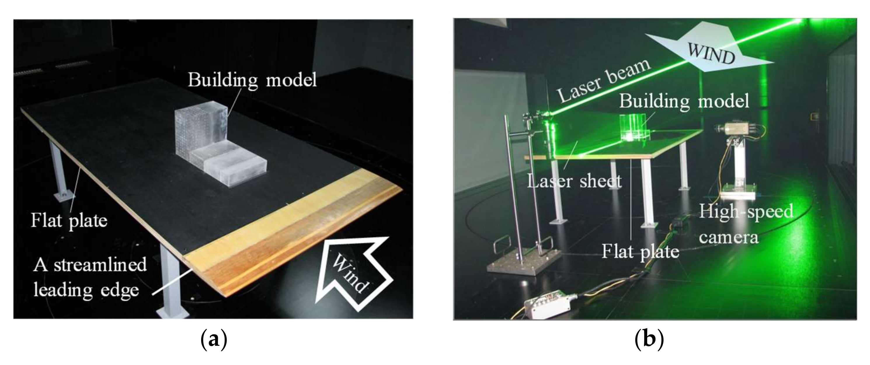
Figure 2.
The definition of the building models and pressure measurement regions. (a) The building referred to as R01; (b) the building referred to as SBL.
Figure 2.
The definition of the building models and pressure measurement regions. (a) The building referred to as R01; (b) the building referred to as SBL.
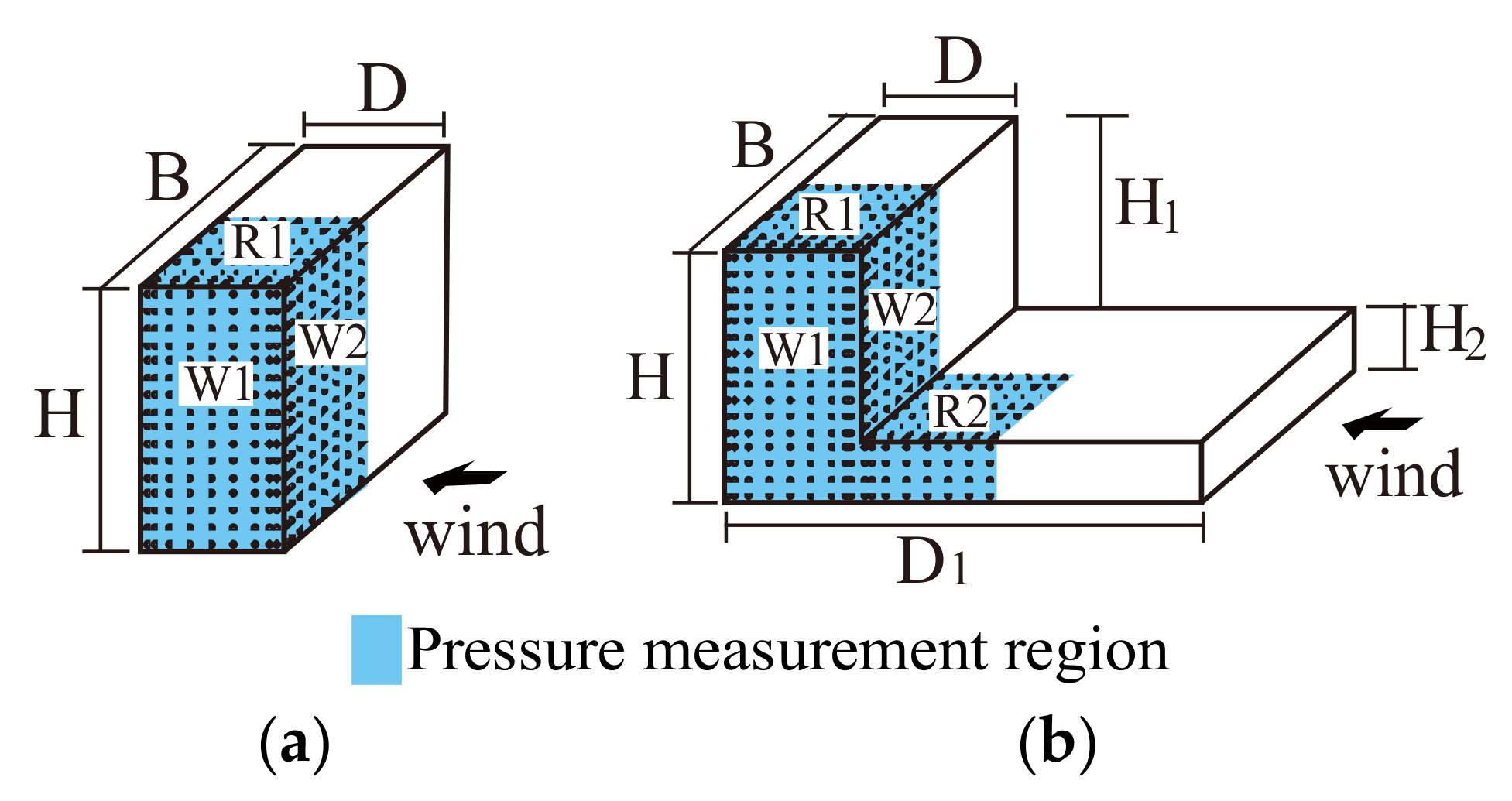
Figure 3.
The definition of the building models and PIV measurement regions. (a) The building R01; (b) the building SBL.
Figure 3.
The definition of the building models and PIV measurement regions. (a) The building R01; (b) the building SBL.
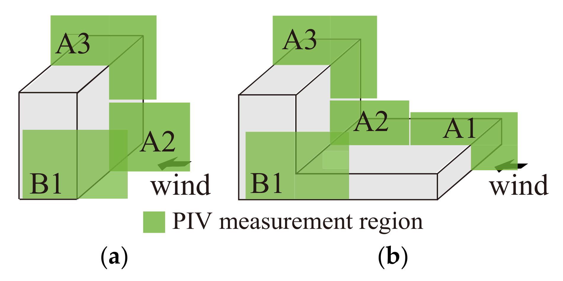
Figure 4.
The computational model and boundary conditions.
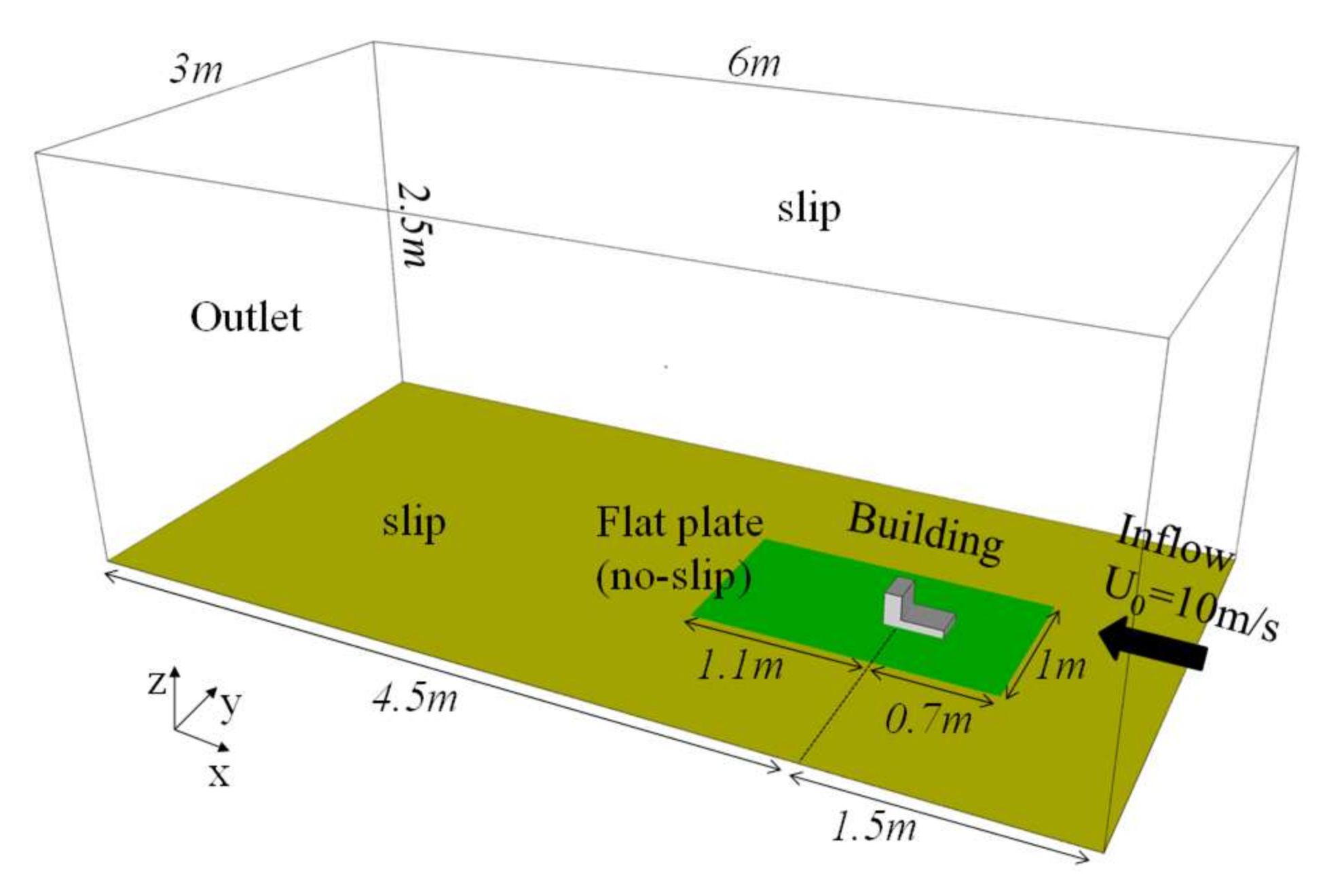
Figure 5.
The computational mesh and its close-up with refinement levels. (a) The entire mesh in plane view; (b) mesh of building R01; (c) mesh of building SBL.
Figure 5.
The computational mesh and its close-up with refinement levels. (a) The entire mesh in plane view; (b) mesh of building R01; (c) mesh of building SBL.

Figure 6.
The pressure distribution on buildings obtained from the pressure experiments. (a) Mean pressure coefficient of R01; (b) negative peak pressure coefficient of R01; (c) mean pressure coefficient of SBL; (d) negative peak pressure coefficient of SBL.
Figure 6.
The pressure distribution on buildings obtained from the pressure experiments. (a) Mean pressure coefficient of R01; (b) negative peak pressure coefficient of R01; (c) mean pressure coefficient of SBL; (d) negative peak pressure coefficient of SBL.
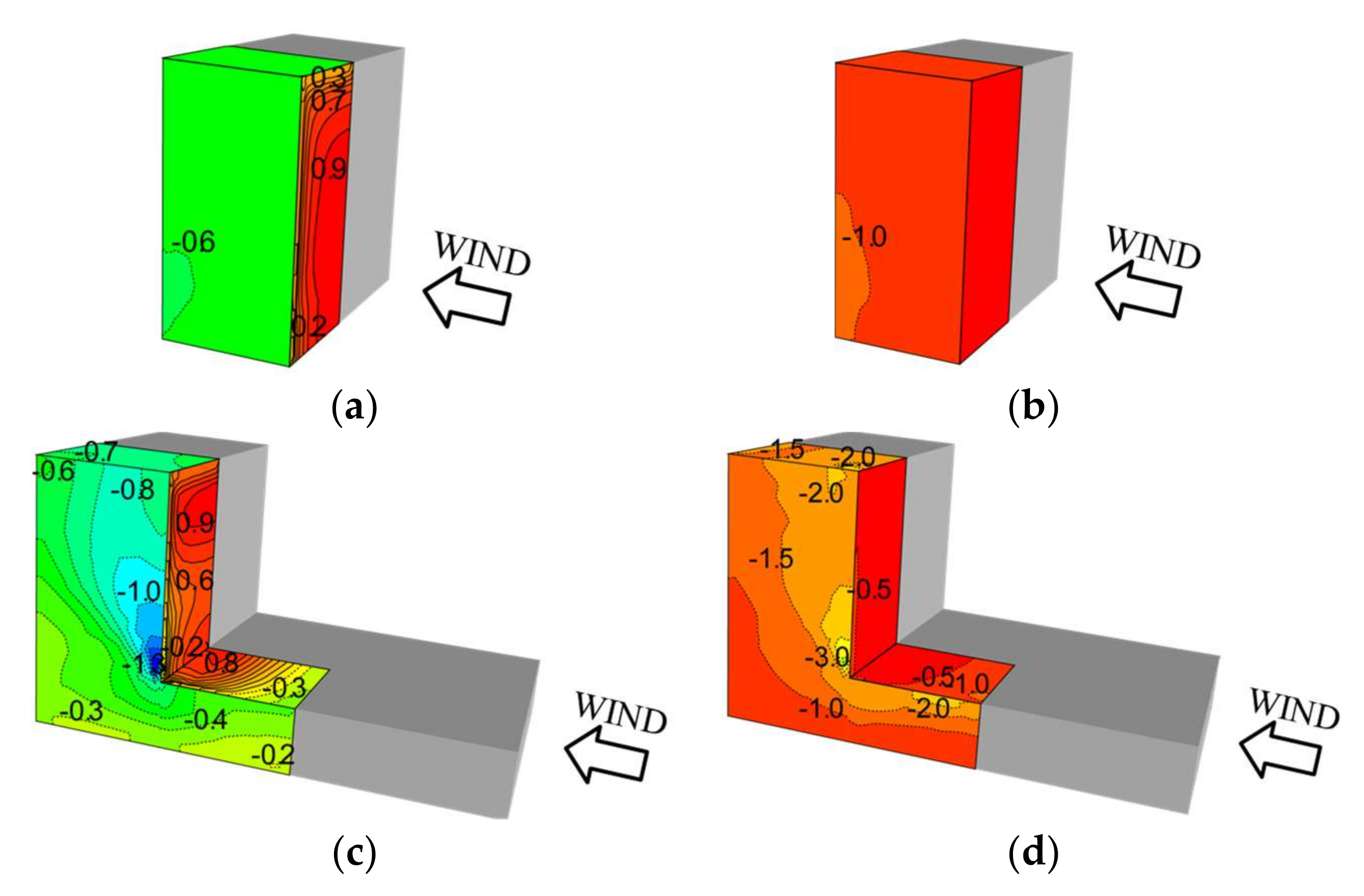
Figure 7.
The pressure coefficients obtained from the SM and CSM with Cr = 2.0 in comparison with experimental results. (a) Mean pressure coefficient of R01; (b) negative peak pressure coefficient of R01; (c) mean pressure coefficient of SBL; (d) negative peak pressure coefficient of SBL.
Figure 7.
The pressure coefficients obtained from the SM and CSM with Cr = 2.0 in comparison with experimental results. (a) Mean pressure coefficient of R01; (b) negative peak pressure coefficient of R01; (c) mean pressure coefficient of SBL; (d) negative peak pressure coefficient of SBL.
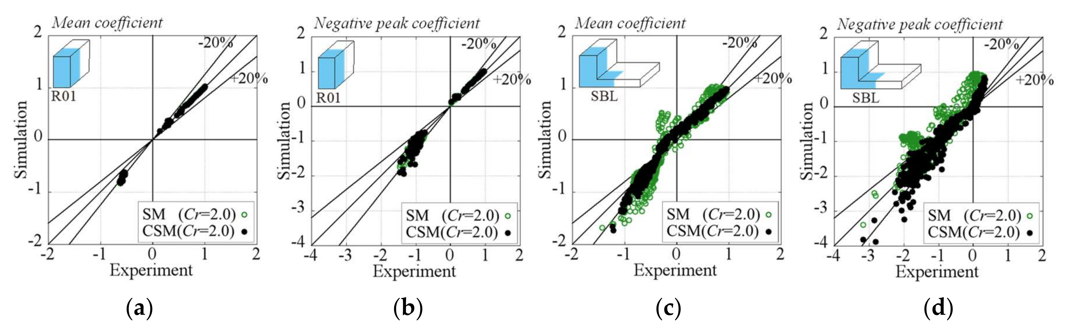
Figure 8.
Pressure coefficients obtained from the CSM with different Cr values. (a) Mean pressure coefficient of R01; (b) negative peak pressure coefficient of R01; (c) mean pressure coefficient of SBL; (d) negative peak pressure coefficient of SBL.
Figure 8.
Pressure coefficients obtained from the CSM with different Cr values. (a) Mean pressure coefficient of R01; (b) negative peak pressure coefficient of R01; (c) mean pressure coefficient of SBL; (d) negative peak pressure coefficient of SBL.
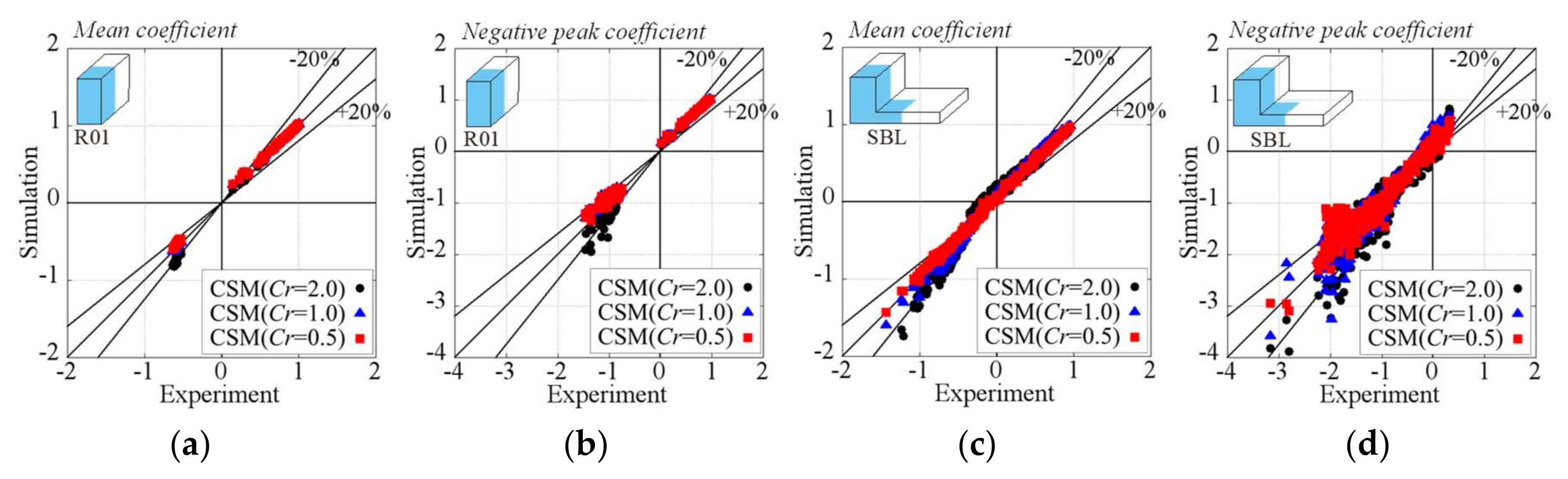
Figure 9.
The mean velocity vector and average vorticity contour obtained by the PIV experiments. (a) The results of building R01 at the central cross section; (b) results of building SBL at the central cross section; (c) results of building R01 at the plane 5 mm away from the sidewall; (d) results of building SBL at the plane 5 mm away from the sidewall.


Figure 10.
The mean streamline around buildings as obtained using the CSM. (a) Building R01; (b) building SBL.
Figure 10.
The mean streamline around buildings as obtained using the CSM. (a) Building R01; (b) building SBL.

Figure 11.
The mean velocity profile in the planes A1, A2, and A3 as obtained by the SM and the CSM in comparison with the PIV experiments. (a) Results of building R01; (b) partially enlarged view of results of building R01; (c) results of building SBL; (d) partially enlarged view of results of building SBL.


Figure 12.
The mean velocity profile in the plane B1, 5 mm away from surface W1, obtained using the SM and the CSM in comparison with the PIV experiments. (a) Results of building R01; (b) partially enlarged view of results of building R01; (c) results of building SBL; (d) partially enlarged view of results of building SBL.
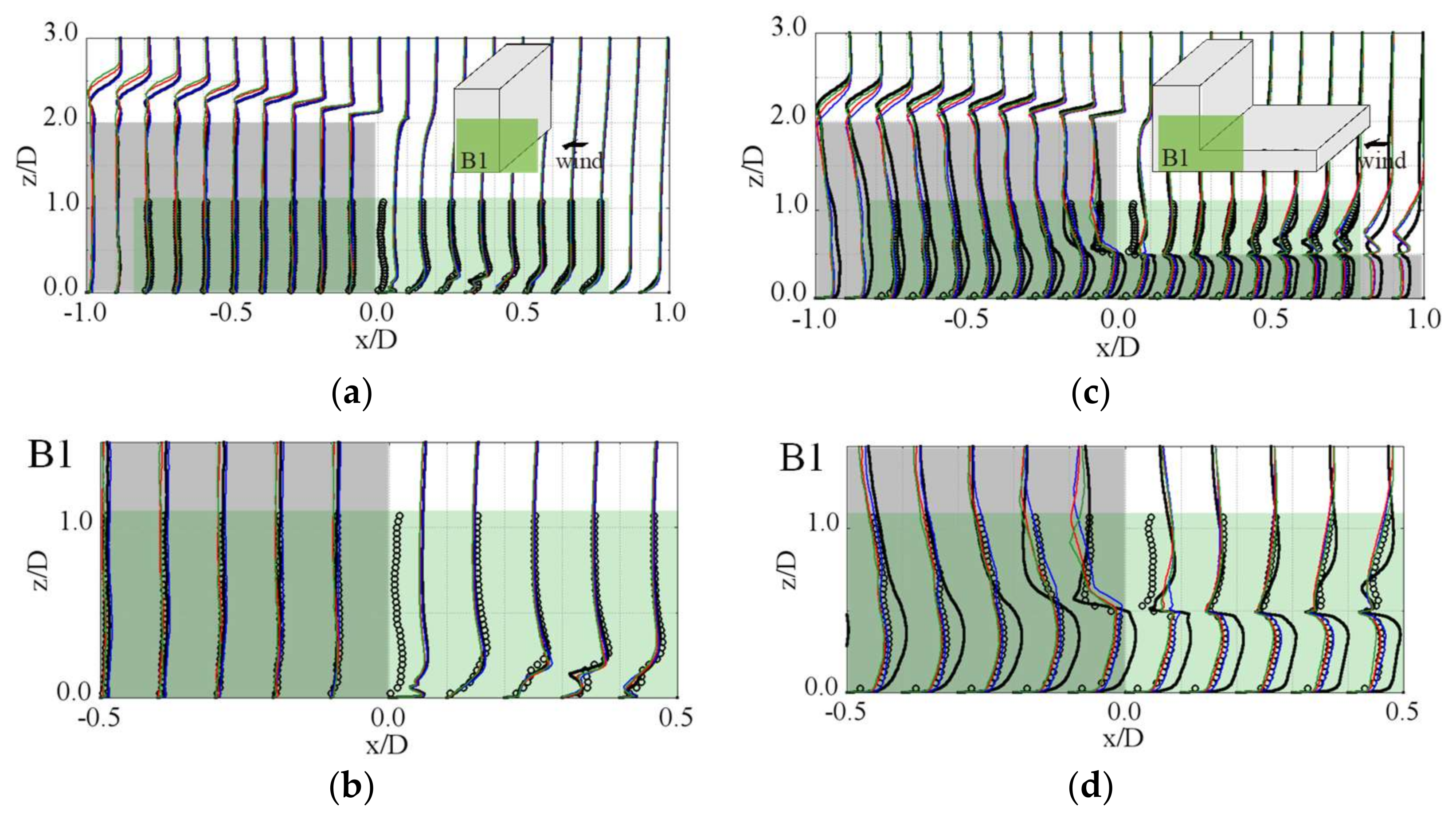
Figure 13.
Wind tunnel experiment. (a) Wind tunnel model setup; (b) target building and pressure measurement point layers.
Figure 13.
Wind tunnel experiment. (a) Wind tunnel model setup; (b) target building and pressure measurement point layers.
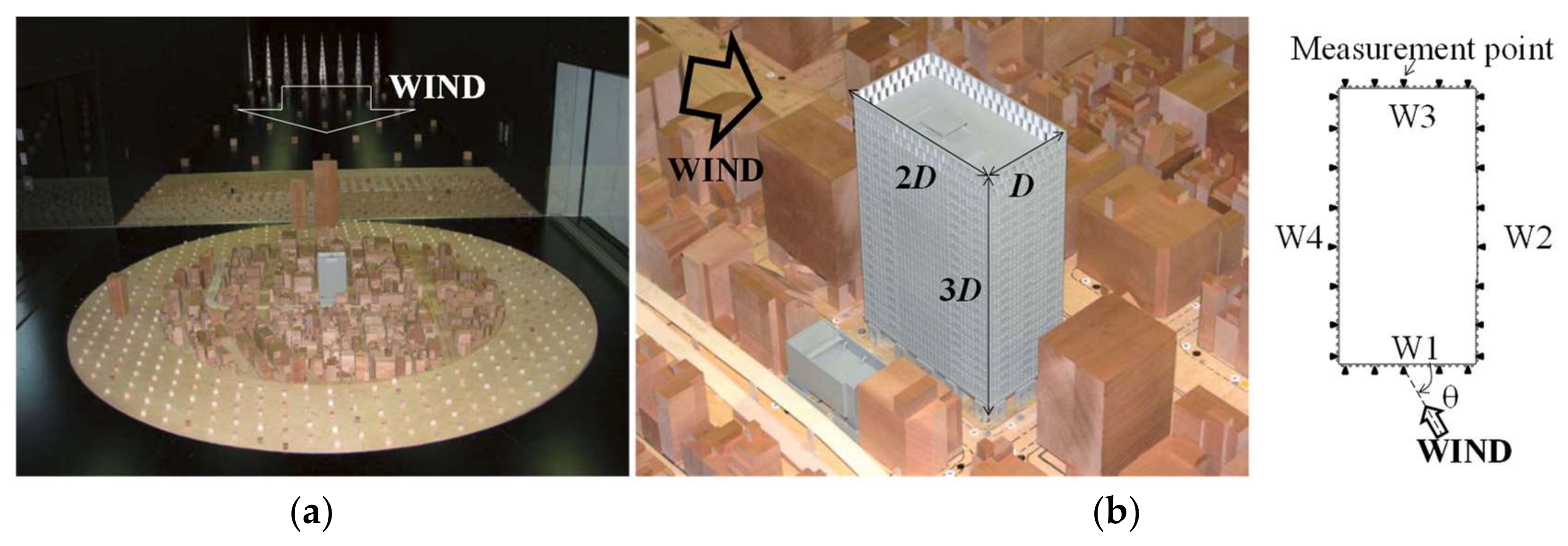
Figure 14.
The computational model and boundary conditions.

Figure 15.
The computational mesh of the spire and roughness blocks with the refinement levels.

Figure 16.
The computational mesh of the building model, its vicinity, and an enlarged view. (a) Mesh A (140 million cells); (b) Mesh B (1.1 billion cells).
Figure 16.
The computational mesh of the building model, its vicinity, and an enlarged view. (a) Mesh A (140 million cells); (b) Mesh B (1.1 billion cells).
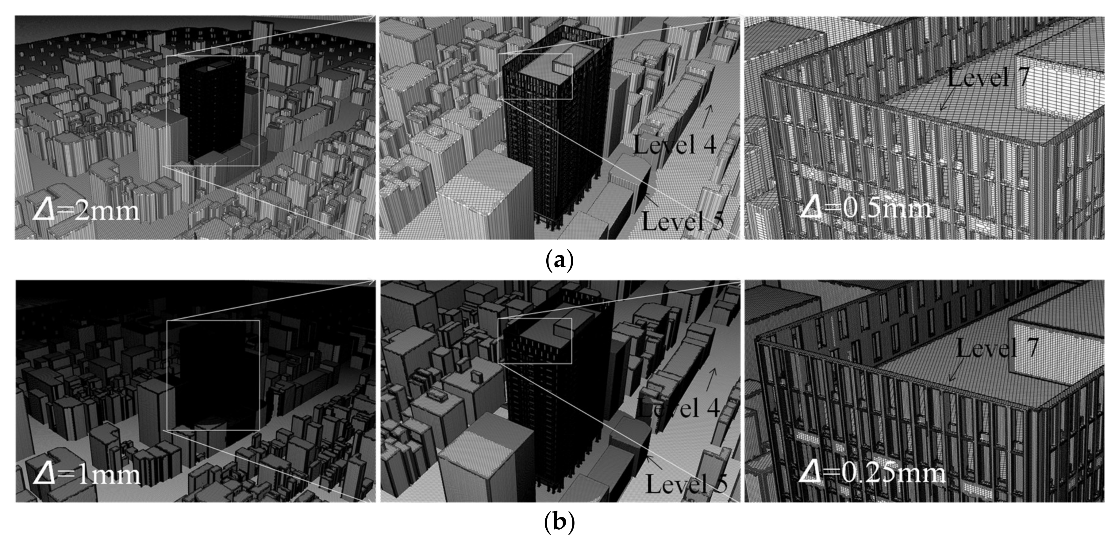
Figure 17.
The wind flow characteristics as obtained by the experiments and LES (Mesh A without buildings). (a) Mean wind speed; (b) longitudinal turbulence intensity, Iu; (c) lateral turbulence intensity, Iv; (d) vertical turbulence intensity, Iw; (e) power spectrum density, Su; (f) power spectrum density, Sv; (g) power spectrum density, Sw.

Figure 18.
The mean wind speed contours. (a) Section z = 0.2H; (b) section z = 0.5H; (c) section z = 0.9H.
Figure 18.
The mean wind speed contours. (a) Section z = 0.2H; (b) section z = 0.5H; (c) section z = 0.9H.

Figure 19.
The flow field around the target building as obtained by the CSM with Mesh A. (a) Mean streamline; (b) instantaneous Q-criterion isosurface (Q = 300,000).
Figure 19.
The flow field around the target building as obtained by the CSM with Mesh A. (a) Mean streamline; (b) instantaneous Q-criterion isosurface (Q = 300,000).

Figure 20.
The mean pressure coefficient. (a) Experimental values; (b) result of the SM with Mesh A; (c) result of the CSM with Mesh A; (d) result of the CSM with Mesh B.
Figure 20.
The mean pressure coefficient. (a) Experimental values; (b) result of the SM with Mesh A; (c) result of the CSM with Mesh A; (d) result of the CSM with Mesh B.
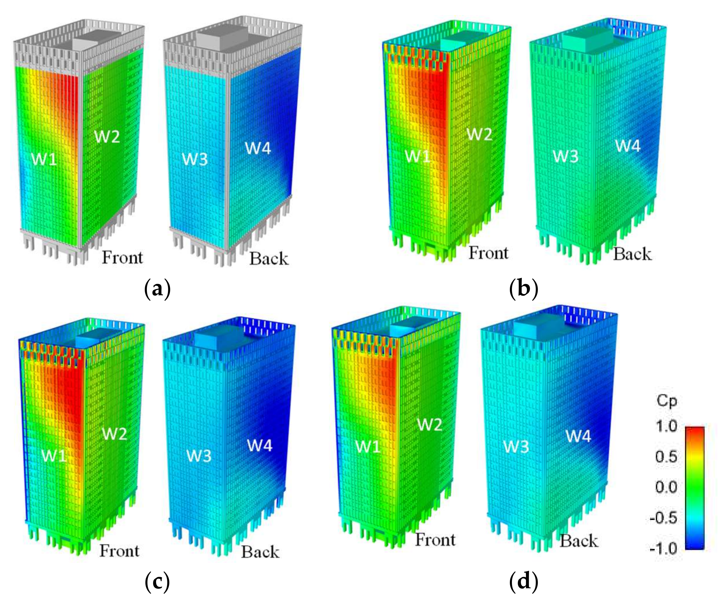
Figure 21.
The comparisons of the mean pressure coefficients between the experiments and LES. (a) Result of the SM with Mesh A; (b) result of the CSM with Mesh A; (c) results of the CSM with Mesh B.
Figure 21.
The comparisons of the mean pressure coefficients between the experiments and LES. (a) Result of the SM with Mesh A; (b) result of the CSM with Mesh A; (c) results of the CSM with Mesh B.
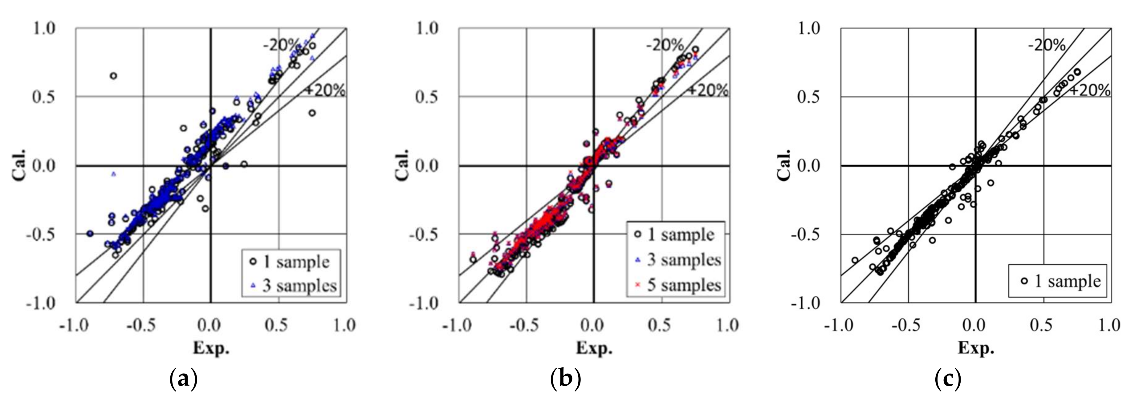
Figure 22.
The comparisons between experiments and LES of the largest negative peak pressure coefficients. (a) SM with Mesh A; (b) results of the CSM with Mesh A; (c) results of the CSM with Mesh B.
Figure 22.
The comparisons between experiments and LES of the largest negative peak pressure coefficients. (a) SM with Mesh A; (b) results of the CSM with Mesh A; (c) results of the CSM with Mesh B.

Figure 23.
The pressure coefficients as obtained by the experiments and LES using CSM (Mesh A, five samples). (a) Mean coefficient; (b) standard deviation coefficient; (c) largest positive peak pressure coefficient; (d) largest negative peak pressure coefficient.
Figure 23.
The pressure coefficients as obtained by the experiments and LES using CSM (Mesh A, five samples). (a) Mean coefficient; (b) standard deviation coefficient; (c) largest positive peak pressure coefficient; (d) largest negative peak pressure coefficient.
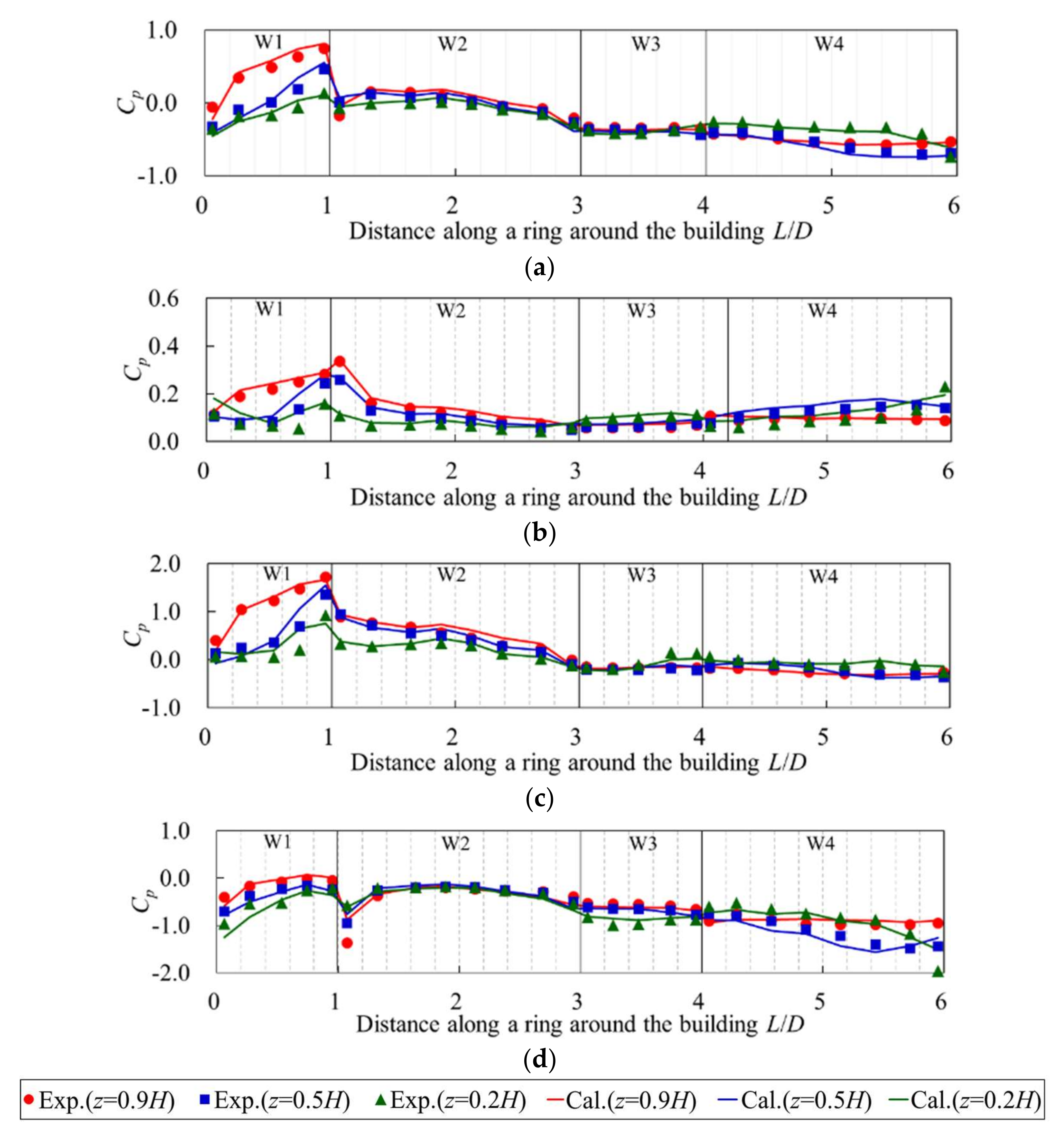
Figure 24.
The comparison of the peak pressure coefficients estimated for all wind directions (CSM, Mesh A). (a) Largest positive peak pressure coefficient; (b) largest negative peak pressure coefficient.
Figure 24.
The comparison of the peak pressure coefficients estimated for all wind directions (CSM, Mesh A). (a) Largest positive peak pressure coefficient; (b) largest negative peak pressure coefficient.

Figure 25.
The pressure coefficients for all wind directions calculated from experiments and LES using the CSM. (a) Largest positive peak pressure coefficient; (b) largest negative peak pressure coefficient.
Figure 25.
The pressure coefficients for all wind directions calculated from experiments and LES using the CSM. (a) Largest positive peak pressure coefficient; (b) largest negative peak pressure coefficient.


Table 1.
The dimensions of the building models in the scale of 1:250 (unit: m).
| Type | B | D | H | H1 | H2 | D1 |
|---|---|---|---|---|---|---|
| R01 | 0.20 | 0.10 | 0.20 | |||
| SBL | 0.20 | 0.10 | 0.20 | 0.15 | 0.05 | 0.35 |
Table 2.
The calculation conditions.
| Subgrid-Scale (SGS) Model | Smagorinsky Model (SM) | Coherent Structure Smagorinsky Model (CSM) |
|---|---|---|
| Mesh cells (millions) | 570 | 570 |
| Time increment Δt (s) | 10−4 | 10−4, 5 × 10⁻⁵, 2.5 × 10⁻⁵ |
| Courant number Cr | 2.0 | 2.0, 1.0, 0.5 |
| Initial run-up time (s) | 3 | 3 |
| Evaluation time (s) | 8 | 8 |
| Number of parallel CPUs | 6144 | 6144 |
Table 3.
The calculation conditions.
| SGS Model Use in Large Eddy Simulation (LES) | SM | CSM | CSM |
|---|---|---|---|
| Mesh type | A | A | B |
| Mesh cells (millions) | 140 | 140 | 1100 |
| Wind direction θ (degree) | 60 | 60 (0, .., 350) | 60 |
| Time increment Δt (s) | 2.5 × 10⁻⁵ | 2.5 × 10⁻⁵ | 1.25 × 10⁻⁵ |
| Courant number Cr | 1 | 1 | 1 |
| Initial run-up time (s) | 3 | 3 | 3 |
| Evaluation time (s) | 18 | 30 (6) | 6 |
| Number of samples in ten-minute record in real-time conversion for evaluation | 3 | 5 (1) | 1 |
| Number of parallel CPUs | 768 | 768 | 6144 |
| Computational time for one sample (days) | 40 | 20 | 20 |
© 2018 by the authors. Licensee MDPI, Basel, Switzerland. This article is an open access article distributed under the terms and conditions of the Creative Commons Attribution (CC BY) license (http://creativecommons.org/licenses/by/4.0/).
Share and Cite
MDPI and ACS Style
Phuc, P.V.; Nozu, T.; Kikuchi, H.; Hibi, K.; Tamura, Y. Wind Pressure Distributions on Buildings Using the Coherent Structure Smagorinsky Model for LES. Computation 2018, 6, 32. https://doi.org/10.3390/computation6020032
AMA Style
Phuc PV, Nozu T, Kikuchi H, Hibi K, Tamura Y. Wind Pressure Distributions on Buildings Using the Coherent Structure Smagorinsky Model for LES. Computation. 2018; 6(2):32. https://doi.org/10.3390/computation6020032
Chicago/Turabian StylePhuc, Pham Van, Tsuyoshi Nozu, Hirotoshi Kikuchi, Kazuki Hibi, and Yukio Tamura. 2018. "Wind Pressure Distributions on Buildings Using the Coherent Structure Smagorinsky Model for LES" Computation 6, no. 2: 32. https://doi.org/10.3390/computation6020032
Note that from the first issue of 2016, this journal uses article numbers instead of page numbers. See further details here.