Modeling the Adaptive Immunity and Both Modes of Transmission in HIV Infection


1
Centre Régional des Métiers de l’Education et de la Formation (CRMEF), 20340 Derb Ghalef, Casablanca, Morocco
2
Laboratory of Analysis, Modeling and Simulation (LAMS), Faculty of Sciences Ben M’sik, Hassan II University, P.O. Box 7955, Sidi Othman, Casablanca, Morocco
*
Author to whom correspondence should be addressed.
Computation 2018, 6(2), 37; https://doi.org/10.3390/computation6020037
Submission received: 15 February 2018
/
Revised: 20 April 2018
/
Accepted: 4 May 2018
/
Published: 8 May 2018
(This article belongs to the Section Computational Biology)
Abstract
:Human immunodeficiency virus (HIV) is a retrovirus that causes HIV infection and over time acquired immunodeficiency syndrome (AIDS). It can be spread and transmitted through two fundamental modes, one by virus-to-cell infection, and the other by direct cell-to-cell transmission. In this paper, we propose a new mathematical model that incorporates both modes of transmission and takes into account the role of the adaptive immune response in HIV infection. We first show that the proposed model is mathematically and biologically well posed. Moreover, we prove that the dynamical behavior of the model is fully determined by five threshold parameters. Furthermore, numerical simulations are presented to confirm our theoretical results.
1. Introduction
Viruses are very small infectious agents that need to penetrate inside a cell of their host to replicate and multiply. Several viruses attack the human body, such as influenza virus, human immunodeficiency virus (HIV), hepatitis B virus (HBV), hepatitis C virus (HCV), Ebola virus, Zika virus, and so on. Viral infections caused by these viruses represent a major global health problem by causing the mortality of millions of people and the expenditure of enormous amounts of money in health care and disease control. In this study, we are interested in the viral infection caused by HIV. The World Health Organization (WHO) estimates that million people were living with HIV at the end of 2016, and more than 1 million people died from HIV-related causes in 2016 [1]. In Morocco, the number of people living with HIV is estimated at 28,740, and 1097 people died from AIDS in 2014, while the cumulative number of HIV/AIDS cases reported since the beginning of the epidemic is 10,017 [2].
Many mathematical models have been developed to better understand the dynamics of HIV infection. One of the earliest of these models was presented by Perelson et al. [3] in 1996. This model is given by the following system:
where , , and are the concentrations of healthy CD4 T cells, infected cells, and free virus at time t, respectively. Healthy cells are produced at rate , die at rate d, and become infected by free virus at rate . The parameter a is the death rate of infected cells. Free virus is produced by an infected cell at rate k and is removed at rate .
In the system given by Equation (1), the cell infection is instantaneous and is caused only by contact with free virus. In reality, there are two kinds of delays: one in cell infection, and the other in virus production. In addition, HIV can spread by two fundamental modes, one by virus-to-cell infection, and the other by direct cell-to-cell transmission. For these above reasons, Lai and Zou [4] improved the model of Perelson et al. [3] by incorporating the two modes of transmission and infinite distributed delay in cell infection. They obtained the following model:
where denotes the rate for a target cell to contact with an infected cell. It is assumed that the virus or infected cell contacts an uninfected target cell at time and the cell becomes infected at time t, where is a random variable taken from a probability distribution . The term represents the probability of surviving from time to time t, where is the death rate for infected but not yet virus-producing cells. The other parameters have the same biological meaning as in Equation (1).
On the other hand, the adaptive immune responses of cytotoxic T lymphocytes (CTLs) and antibodies play an important role in the control of HIV infection. The first immune response exerted by CTL cells is called the cellular immunity. However, the second immune response mediated by antibodies is called the humoral immunity. In the literature, several authors are interested in modeling the role of these arms of immunity in viral infections. In 2016, Wang et al. [5] improved the model given by Equation (2) by considering the role of cellular immune response. In the same year, Elaiw et al. [6] improved the model given by Equation (2) by considering only the role of humoral immune response and infinite distributed delay in virus production. In 2017, Lin et al. [7] improved the models of Wang and Zou [8] and Murase et al. [9] by incorporating both modes of transmission, intracellular delay and humoral immunity.
The aim of this work is to improve and generalize all the above models by proposing a new mathematical model that takes into account the role of the adaptive immune response in HIV infection and incorporates both modes of transmission. To this end, the next section deals with the presentation of our model and some properties of solutions, such as positivity and boundedness. In Section 2, we derive the threshold parameters of our model and discuss the existence of equilibria. The global stability of equilibria is investigated in Section 3. Some numerical simulations of our main results are presented in Section 4. The mathematical and biological conclusions are given in Section 5.
2. Presentation of the Model
To model the role of the adaptive immune response in HIV infection with both virus-to-cell infection and cell-to-cell transmission, we propose the following model:
where and are the concentrations of antibodies and CTL cells at time t, respectively. Free HIV particles are neutralized by the antibodies at rate . However, the infected cells are killed by CTL cells at rate . Antibodies develop in response to free virus at rate , and CTL cells expand in response to viral antigens derived from infected cells at rate . The parameters h and b are, respectively, the death rates of antibodies and CTL cells. Further, we assume that the time necessary for the newly produced virions to become mature and infectious is a random variable with a probability distribution . The term denotes the probability of surviving the immature virions during the delay period, where is the average lifetime of an immature virus. Therefore, the integral describes the mature viral particles produced at time t. The other variables and parameters are defined as those in the systems given by Equations (1) and (2).
In this section, we first investigate the nonnegativity and boundedness of solutions under the following nonnegative initial conditions:
We define the Banach space for the fading memory type as follows:
where is a positive constant and .
Theorem 1.
Proof.
By the fundamental theory of functional differential equations [10,11,12], the model given by Equation (3) with initial condition has a unique local solution on , where is the maximal existence time for the solution of Equation (3).
First, we prove that for all . In fact, supposing the contrary, we let be the first time such that and . By the first equation of the model given by Equation (3), we have , which is a contradiction. Thus, for all . By Equation (3), we have
which implies that , , , and are nonnegative for all .
Next, we show the boundedness of each solution. From the first equation of the model given by Equation (3), we have , which implies that
Then is bounded. Let
Because is bounded and , the integral in is well defined and differentiable with respect to t. Hence,
where and
Thus, , which implies that and are bounded. It remains to prove that and are bounded. To this end, we consider
then
where . Similarly to the above, we deduce that and are also bounded. We have proved that all variables of Equation (3) are bounded, which implies that and that the solution exists globally. ☐
If in addition to Equation (4), we suppose that for all ; then we obtain the following remark.
Remark 1.
Next, we derive threshold numbers and identify biological equilibria for the model given by Equation (3). Clearly, Equation (3) always has an infection-free equilibrium of the form , where . Therefore, the basic reproduction number of Equation (3) can be defined as
As in [13], can be rewritten as , where is the basic reproduction number corresponding to the virus-to-cell infection mode, and is the basic reproduction number corresponding to the cell-to-cell transmission mode.
When , Equation (3) has another infection equilibrium without immunity, , where
If both humoral and cellular immune responses have not been established, we have and . Thus, we define the reproduction number for humoral immunity:
and the reproduction number for cellular immunity:
Hence, and are equivalent to and , respectively.
When , Equation (3) has an infection equilibrium with only humoral immunity, , where
with , , and .
It is not hard to see that , and are positive. It remains to check that is positive. Because and
we easily deduce that . If cellular immunity has not been established, we have . For this, we define the reproduction number for cellular immunity in competition as
which implies that is equivalent to .
When , Equation (3) has an infection equilibrium with only cellular immunity, , where
We have that , , and are positive. It suffices to check that is positive. Because and
we deduce that . If humoral immunity has not been established, we have . In this case, we define the reproduction number for humoral immunity in competition as
which implies that is equivalent to .
When and , Equation (3) has an infection equilibrium with both cellular and humoral immune responses, , where
We have , , , and (as ). It remains to check that . On the other hand, is equivalent to . By a simple computation, we have
Summarizing the above discussions, we obtain the following theorem.
Theorem 2.
- (i)
- If , then Equation (3) always has one infection-free equilibrium, , where .
- (ii)
- If , then Equation (3) has an infection equilibrium without immunity, , where
- (iii)
- If , then Equation (3) has an infection equilibrium with only humoral immunity, , where
- (iv)
- If , then Equation (3) has an infection equilibrium with only cellular immunity, , where
- (v)
- If and , then Equation (3) has an infection equilibrium with both cellular and humoral immune responses, , where
It is important to note that
3. Global Stability
In this section, we investigate the global stability of the five equilibria of Equation (3) by constructing appropriate Lyapunov functionals. We first analyze the global stability of the infection-free equilibrium.
Theorem 3.
The infection-free equilibrium is globally asymptotically stable when .
Proof.
To study the global stability of , we consider a Lyapunov functional defined as follows:
where for . It is not hard to see that for all . Hence, the functional is nonnegative.
In order to simplify the presentation, we use the following notations: and for any . Calculating the time derivative of along the positive solution of Equation (3), we obtain
If follows from that . It is straightforward to show that the largest invariant set in is . By LaSalle’s invariance principle [14], the infection-free equilibrium is globally asymptotically stable when . ☐
When , Equation (3) has four infection steady states , . The following theorem characterizes the global stability of these steady states.
Theorem 4.
Assume .
- (i)
- The infection equilibrium without immunity is globally asymptotically stable if and .
- (ii)
- The infection equilibrium with only humoral immunity is globally asymptotically stable if and .
- (iii)
- The infection equilibrium with only cellular immunity is globally asymptotically stable if and .
- (iv)
- The infection equilibrium with both cellular and humoral immune responses is globally asymptotically stable if and .
Proof.
For (i), consider the following Lyapunov functional:
Then
By and , we obtain
Thus,
Because for , , and , we have with equality if and only if , , , , and . It follows from LaSalle’s invariance principle that is globally asymptotically stable.
For (ii), consider the following Lyapunov functional:
Hence,
By , , and , we obtain
Thus,
Because and for , we have with equality if and only if , , and . Then and , which leads to and . Therefore, the largest compact invariant set in is the singleton , and the proof of (ii) is completed.
For (iii), consider the following Lyapunov functional:
From , , and , we easily have
Consequently, with equality if and only if , , and . It follows from and that and . By LaSalle’s invariance principle, we deduce that is globally asymptotically stable.
Finally, we show (iv) by considering the following Lyapunov functional:
By , , and , we obtain
Hence,
Thus, with equality holds if and only if , , and . Let
From the second and third equations of the model given by Equation (3), we have
which implies that and . Then the largest compact invariant set in is the singleton . Therefore, is globally asymptotically stable. ☐
The conditions of the global stability of and those of given in (ii) and (iii) of Theorem 4 do not hold simultaneously. In fact, supposing the contrary, then and . Because and , we have . This is a contradiction with .
According to Equation (12) and Theorem 4, we have the following important result.
Remark 2.
Assume .
From this important remark, we can define the over-domination of humoral immunity when and and the over-domination of cellular immunity when and .
4. Numerical Simulations
In this section, we present some numerical simulations in order to validate our theoretical results. For simplicity, we chose and with and to be the delays in cell infection and virus production, respectively, and to be the Dirac function; then our model becomes
This system improves the model presented in 2017 by Lin et al. [7], which considered only the humoral immunity and discrete delay in cell infection and ignored the time delay in virus production; that is, . In addition, Equation (13) includes many special cases existing in the literature. For example, when and , we obtain the model presented by Wodarz in [15] and analyzed by Hattaf et al. in [16]. When and , we obtain the model of Yan and Wang [17].
The algorithm for the numerical treatment of the delay differential system given by Equation (13) can be derived for the numerical method presented in [18,19]. Recently, this numerical method has been used for delayed partial differential equations [20]; it is called the “mixed” Euler method, as it is a mixture of both forward and backward Euler methods. In addition, it is shown that this mixed Euler method preserves the qualitative properties of the corresponding continuous system, such as positivity, boundedness, and global behaviors of solutions. Hence, we discretize the continuous system given by Equation (13) by this numerical method. Thus, we let be a time step size and assume that there exist two integers with and . The grids points are for . By applying the mixed Euler method and using the approximations , , , , and , we obtain the following discrete model:
where the discrete initial conditions are
The five threshold parameters , , , , and for Equation (13) are given by Equations (7)–(11) with and . In order to study the impact of cell-to-cell transmission and both arms of adaptive immunity on the HIV dynamics, we chose , g, and c as free parameters. The units of state variables T, I, and Z were given by cells . Further, the units of V and W were given by virions and molecules , respectively. The other parameter values for the simulation are listed in Table 1.
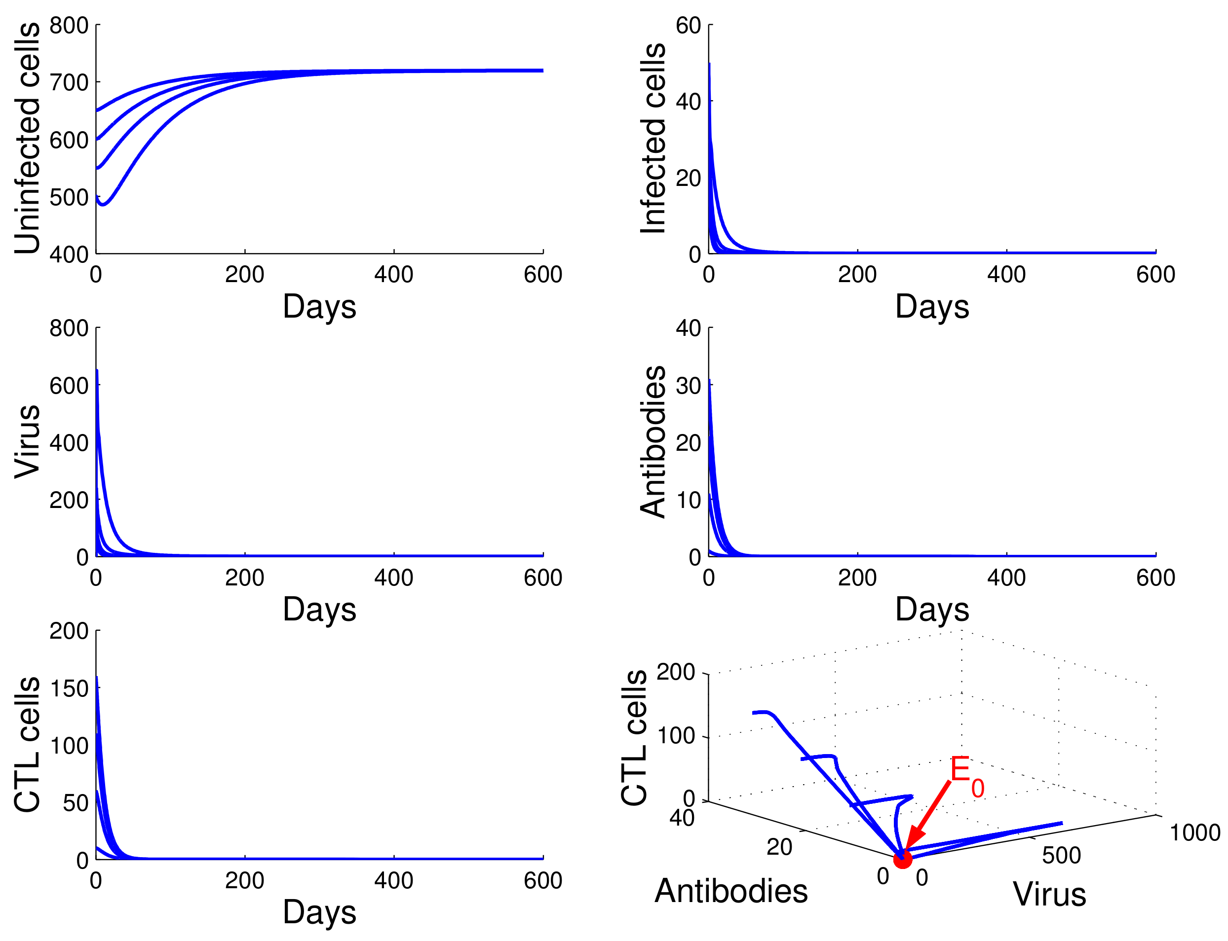
For the case in which , , and , we obtained . It follows from Theorem 2 that Equation (13) has one infection-free equilibrium . From Figure 1, we see that the concentration of uninfected CD4 T cells increased and tended to the value , while the concentrations of infected cells, free HIV particles, antibodies, and CTL cells decreased and tended to zero. This means that is globally asymptotically stable and that the virus will be cleared. This confirms the result in Theorem 3.
For the case in which , , and , we obtained , , and . It follows that case of Theorem 4 occurs, and the infection equilibrium without immunity is globally asymptotically stable (see Figure 2).
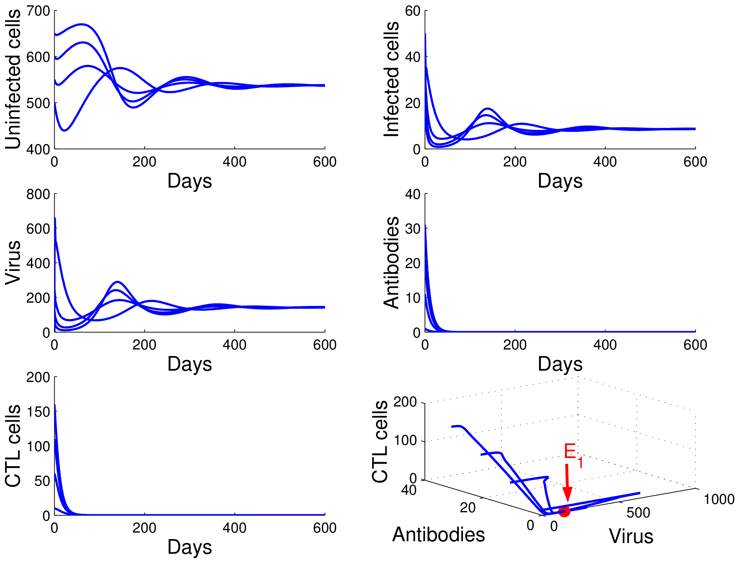
For the case in which , , and , we obtained , , and . From of Theorem 4, the infection equilibrium with only humoral immunity is globally asymptotically stable (see Figure 3).
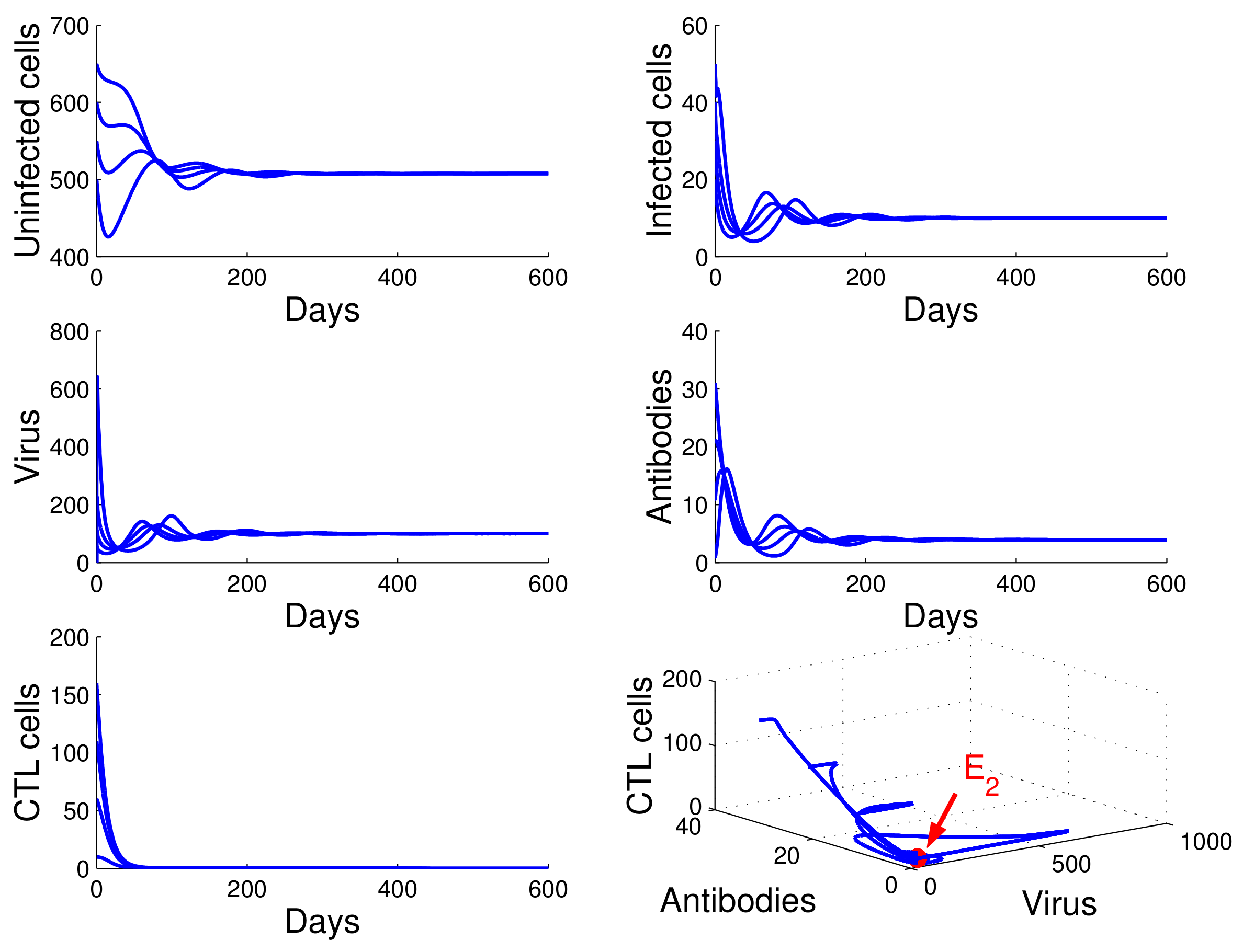
For the case in which , , and , we obtained , , and . By of Theorem 4, the infection equilibrium with only cellular immunity is globally asymptotically stable (see Figure 4).
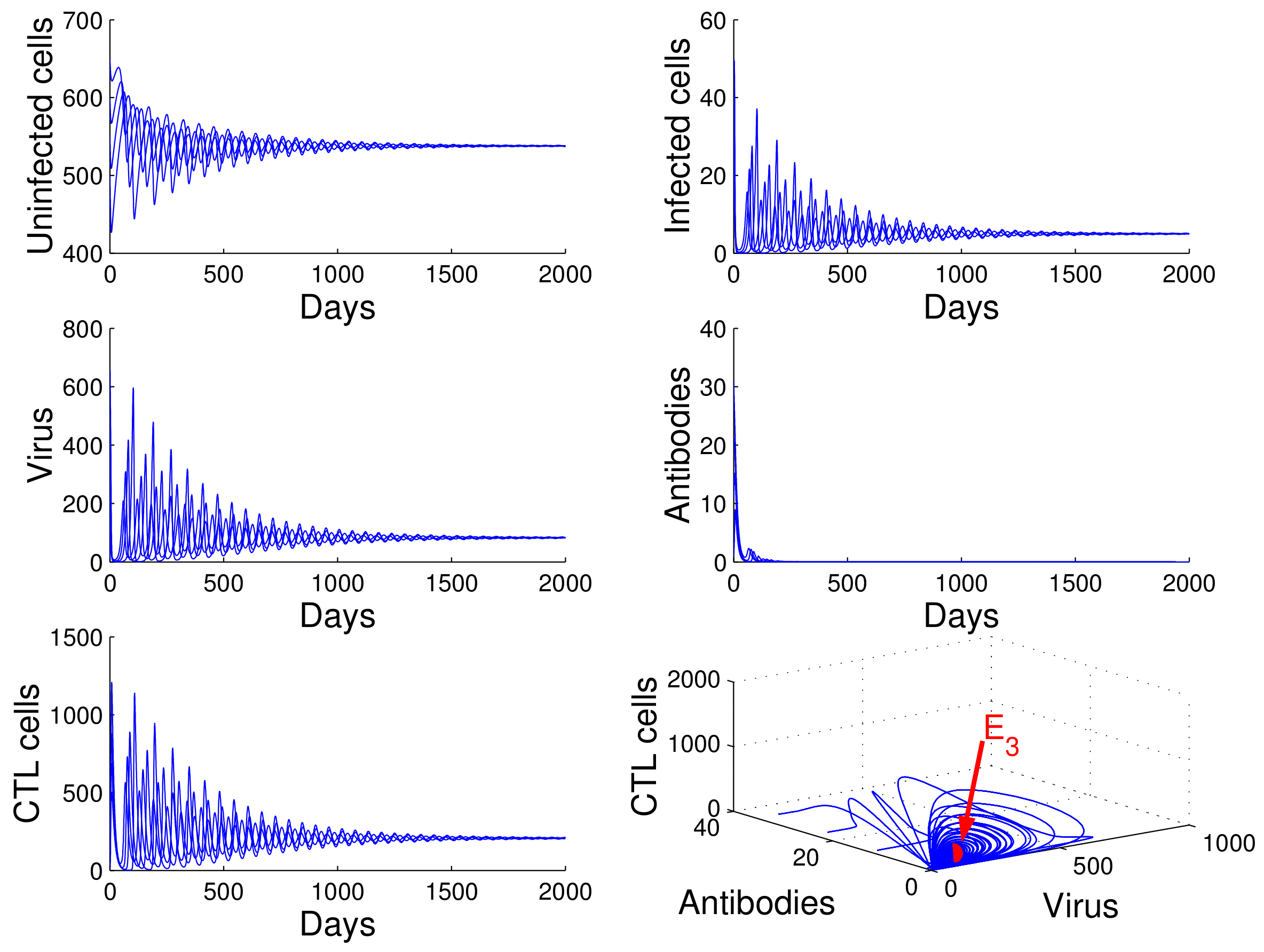
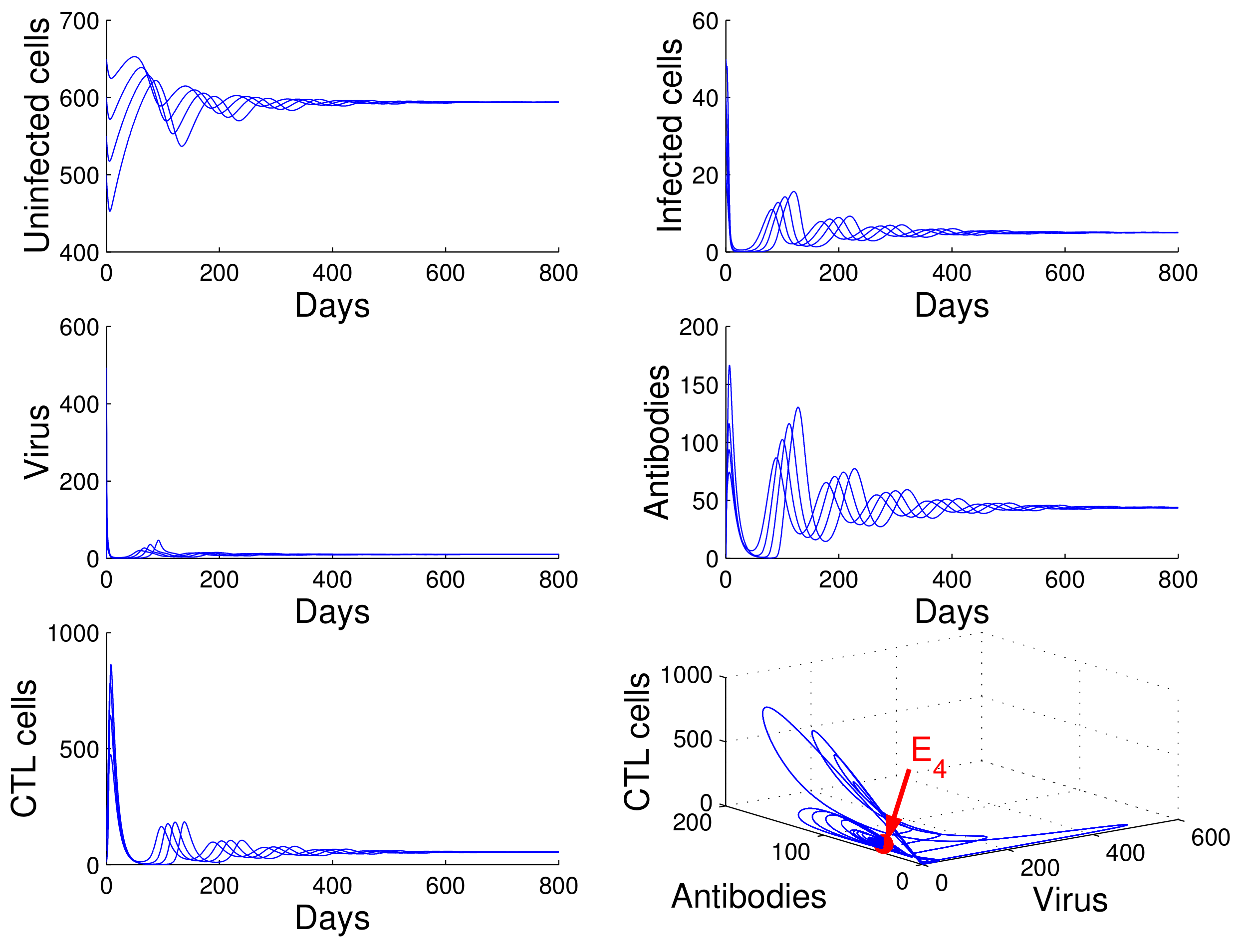
For the case in which , , and , we obtained , , and . Using of Theorem 4, we deduce that the infection equilibrium with both arms of immunity is globally asymptotically stable (see Figure 5).
5. Conclusions
In this paper, we have modeled the role of the adaptive immunity in HIV infection by proposing a new mathematical model that takes into account the classical virus-to-cell infection, the direct cell-to-cell transmission, and the two kinds of delays during infection processes and virus production. By a rigorous mathematical analysis, we have proved that the global dynamics of the proposed model is fully determined by five threshold parameters, which are the basic reproduction number , and the reproduction numbers for humoral immunity , for cellular immunity , for cellular immunity in competition , and for humoral immunity in competition . More precisely, the infection-free equilibrium is globally asymptotically stable if , which biologically means that the HIV is cleared and the infection dies out. When , our model has four infection equilibria, which are the following: the infection equilibrium without immunity is globally asymptotically stable if and ; the infection equilibrium with only humoral immunity is globally asymptotically stable if and ; the infection equilibrium with only cellular immunity is globally asymptotically stable if and ; the infection equilibrium with both cellular and humoral immune responses is globally asymptotically stable if and . Biologically, this implies that the HIV persists and the infection becomes chronic when the basic reproduction number is greater than 1. Additionally, the activation of one or both arms of immunity is unable to eliminate the virus in the human body.
From Remark 2, we can deduce that the over-domination of cellular immunity leads to the absence of the humoral immunity, and the over-domination of the humoral immunity leads to the persistence of HIV infection with a weak response of both arms of immunity. This biological result may be an explanation for the dysfunction of the adaptive immunity in HIV-infected patients. Our model can be adapted for HBV infection, and the above result can also explain the dysfunction of the adaptive immune response in patients infected with HBV, which is still largely incomplete [33].
Author Contributions
Both authors contributed equally to the writing of this paper. They both read and approved the final version of the manuscript.
Acknowledgments
We would like to thank the editor and anonymous referees for their very helpful comments and suggestions that greatly improved the quality of this study.
Conflicts of Interest
The authors declare no conflict of interest.
References
- WHO. HIV/AIDS, Fact Sheet, July 2017. Available online: http://www.who.int/mediacentre/factsheets/fs360/en/ (accessed on 8 May 2018).
- Royaume du Maroc, Mise en oeuvre de la déclaration politique sur le VIH/sida, Rapport National 2015. Available online: http://www.unaids.org/sites/default/files/country/documents/MARnarrativereport2015.pdf (accessed on 8 May 2018).
- Perelson, A.S.; Neumann, A.U.; Markowitz, M.; Leonard, J.M.; Ho, D.D. HIV-1 dynamics in vivo: Virion clearance rate, infected cell life-span, and viral generation time. Science 1996, 271, 1582–1586. [Google Scholar] [CrossRef] [PubMed]
- Lai, X.; Zou, X. Modeling HIV-1 virus dynamics with both virus-to-cell infection and cell-to-cell transmission. SIAM J. Appl. Math. 2014, 74, 898–917. [Google Scholar] [CrossRef]
- Wang, J.; Guo, M.; Liu, X.; Zhao, Z. Threshold dynamics of HIV-1 virus model with cell-to-cell transmission, cell-mediated immune responses and distributed delay. Appl. Math. Comput. 2016, 291, 149–161. [Google Scholar] [CrossRef]
- Elaiw, A.M.; Raezah, A.A.; Alofi, A.S. Effect of humoral immunity on HIV-1 dynamics with virus-to-target and infected-to-target infections. AIP Adv. 2016, 6, 085204. [Google Scholar] [CrossRef]
- Lin, J.; Xu, R.; Tian, X. Threshold dynamics of an HIV-1 virus model with both virus-to-cell and cell-to-cell transmissions, intracellular delay, and humoral immunity. Appl. Math. Comput. 2017, 315, 516–530. [Google Scholar] [CrossRef]
- Wang, S.F.; Zou, D.Y. Global stability of in-host viral models with humoral immunity and intracellular delays. Appl. Math. Model. 2012, 36, 1313–1322. [Google Scholar] [CrossRef]
- Murase, A.; Sasaki, T.; Kajiwara, T. Stability analysis of pathogen-immune interaction dynamics. J. Math. Biol. 2005, 51, 247–267. [Google Scholar] [CrossRef] [PubMed]
- Hale, J.K.; Kato, J. Phase space for retarded equations with infinite delay. Funkcialaj Ekvacioj 1978, 21, 11–41. [Google Scholar]
- Hino, Y.; Murakami, S.; Naito, T. Functional Differential Equations with Infinite Delay; Lecture Notes in Mathematics; Springer: Berlin, Germany, 1991; Volume 1473. [Google Scholar]
- Kuang, Y. Delay Differential Equations with Applications in Population Dynamics; Academic Press: San Diego, CA, USA, 1993. [Google Scholar]
- Hattaf, K.; Yousfi, N. A generalized virus dynamics model with cell-to-cell transmission and cure rate. Adv. Differ. Equ. 2016, 2016, 174. [Google Scholar] [CrossRef]
- Hale, J.K.; Lunel, S.M.V. Introduction to Functional Differential Equations; Springer: New York, NY, USA, 1993. [Google Scholar]
- Wodarz, D. Hepatitis C virus dynamics and pathology: The role of CTL and antibody responses. J. Gen. Virol. 2003, 84, 1743–1750. [Google Scholar] [CrossRef] [PubMed]
- Yousfi, N.; Hattaf, K.; Rachik, M. Analysis of a HCV model with CTL and antibody responses. Appl. Math. Sci. 2009, 3, 2835–2845. [Google Scholar]
- Yan, Y.; Wang, W. Global stability of a five-dimensionalmodel with immune responses and delay. Discret. Contin. Dyn. Syst. Ser. B 2012, 1, 401–416. [Google Scholar]
- Hattaf, K.; Yousfi, N. Global properties of a discrete viral infection model with general incidence rate. Math. Methods Appl. Sci. 2016, 39, 998–1004. [Google Scholar] [CrossRef]
- Hattaf, K.; Yousfi, N. A numerical method for a delayed viral infection model with general incidence rate. J. King Saud Univ. Sci. 2016, 28, 368–374. [Google Scholar] [CrossRef]
- Hattaf, K.; Yousfi, N. A numerical method for delayed partial differential equations describing infectious diseases. Comput. Math. Appl. 2016, 72, 2741–2750. [Google Scholar] [CrossRef]
- Maziane, M.; Lotfi, E.M.; Hattaf, K.; Yousfi, N. Dynamics of a class of HIV infection models with cure of infected cells in eclipse stage. Acta Biotheor. 2015, 63, 363–380. [Google Scholar] [CrossRef] [PubMed]
- Bourgeois, C.; Hao, Z.; Rajewsky, K.; Potocnik, A.; Stockinger, B. Ablation of thymic export causes accelerated decay of naive CD4 T cells in the periphery because of activation by environmental antigen. Proc. Natl. Acad. Sci. USA 2008, 105, 8691–8696. [Google Scholar] [CrossRef] [PubMed]
- Stafford, M.; Corey, L.; Cao, Y.; Daar, E.; Ho, D.; Perelson, A. Modeling plasma virus concentration during primary HIV infection. J. Theor. Biol. 2000, 203, 285–301. [Google Scholar] [CrossRef] [PubMed]
- Wei, X.; Ghosh, S.K.; Taylor, M.E.; Johnson, V.A.; Emini, E.A.; Deutsch, P.; Lifson, J.D.; Bonhoeffer, S.; Nowak, M.A.; Hahn, B.H.; et al. Viral dynamics in human immunodeficiency virus type 1 infection. Nature 1995, 373, 117–122. [Google Scholar] [CrossRef] [PubMed]
- Ho, D.D.; Neumann, A.U.; Perelson, A.S.; Chen, W.; Leonard, J.M.; Markowitz, M. Rapid turnover of plasma virions and CD4 lymphocytes in HIV-1 infection. Nature 1995, 373, 123–126. [Google Scholar] [CrossRef] [PubMed]
- Miao, H.; Teng, Z.; Li, Z. Global Stability of Delayed Viral Infection Models with Nonlinear Antibody and CTL Immune Responses and General Incidence Rate. Comput. Math. Methods Med. 2016, 2016, 3903726. [Google Scholar] [CrossRef] [PubMed]
- Arnaout, R.; Ramy, A.; Wodarz, D. HIV-1 dynamics revisited: biphasic decay by cytotoxic T lymphocyte killing? Proc. R. Soc. Lond. B Biol. Sci. 2000, 267, 1347–1354. [Google Scholar] [CrossRef] [PubMed]
- Culshaw, R.V.; Ruan, S.; Spiteri, R.J. Optimal HIV treatment by maximising immune response. J. Math. Biol. 2004, 48, 545–562. [Google Scholar] [CrossRef] [PubMed]
- Nowak, M.A.; Bangham, C. Population dynamics of immune response to persistent viruses. Science 1996, 272, 74–79. [Google Scholar] [CrossRef] [PubMed]
- Wang, Y.; Zhou, Y.; Brauer, F.; Heffernan, J. Viral dynamics model with CTL immune response incorporating antiretroviral therapy. J. Math. Biol. 2013, 67, 901–934. [Google Scholar] [CrossRef] [PubMed]
- Wang, Y.; Zhou, Y.; Wu, J.; Heffernan, J. Oscillatory viral dynamics in a delayed HIV pathogenesis model. Math. Biosci. 2009, 219, 104–112. [Google Scholar] [CrossRef] [PubMed]
- Zhu, H.; Zou, X. Impact of delays in cell infection and virus production on HIV-1 dynamics. Math. Med. Biol. 2008, 25, 99–112. [Google Scholar] [CrossRef] [PubMed]
- Boni, C.; Fisicaro, P.; Valdatta, C.; Amadei, B.; di Vincenzo, P.; Giuberti, T.; Laccabue, D.; Zerbini, A.; Cavalli, A.; Missale, G.; et al. Characterization of HBV-specific T cell dysfunction in chronic HBV infection. J. Virol. 2007, 8, 4215–4225. [Google Scholar] [CrossRef] [PubMed]
Figure 1.
Demonstration of the global stability of the infection-free equilibrium for .

Figure 2.
Demonstration of the global stability of the infection equilibrium without immunity for , , and .
Figure 2.
Demonstration of the global stability of the infection equilibrium without immunity for , , and .

Figure 3.
Demonstration of the global stability of the infection equilibrium with only humoral immunity for , , and .
Figure 3.
Demonstration of the global stability of the infection equilibrium with only humoral immunity for , , and .

Figure 4.
Demonstration of the global stability of the infection equilibrium with only cellular immunity for , , and .
Figure 4.
Demonstration of the global stability of the infection equilibrium with only cellular immunity for , , and .

Figure 5.
Demonstration of the global stability of the infection equilibrium with both arms of immunity for , , and .
Figure 5.
Demonstration of the global stability of the infection equilibrium with both arms of immunity for , , and .


© 2018 by the authors. Licensee MDPI, Basel, Switzerland. This article is an open access article distributed under the terms and conditions of the Creative Commons Attribution (CC BY) license (http://creativecommons.org/licenses/by/4.0/).
Share and Cite
MDPI and ACS Style
Hattaf, K.; Yousfi, N. Modeling the Adaptive Immunity and Both Modes of Transmission in HIV Infection. Computation 2018, 6, 37. https://doi.org/10.3390/computation6020037
AMA Style
Hattaf K, Yousfi N. Modeling the Adaptive Immunity and Both Modes of Transmission in HIV Infection. Computation. 2018; 6(2):37. https://doi.org/10.3390/computation6020037
Chicago/Turabian StyleHattaf, Khalid, and Noura Yousfi. 2018. "Modeling the Adaptive Immunity and Both Modes of Transmission in HIV Infection" Computation 6, no. 2: 37. https://doi.org/10.3390/computation6020037
Note that from the first issue of 2016, this journal uses article numbers instead of page numbers. See further details here.