An Open-Source Toolbox for PEM Fuel Cell Simulation


1
International Doctoral Innovation Centre, University of Nottingham Ningbo China, 199 Taikang East Road, Ningbo 315100, China
2
Research Centre for Fluids and Thermal Engineering, University of Nottingham Ningbo China, 199 Taikang East Road; Ningbo 315100, China
3
Fluids & Thermal Engineering Research Group, University of Nottingham, University Park, Nottingham NG7 2RD, UK
4
Department of Chemical and Environmental Engineering, University of Nottingham Ningbo China, Ningbo 315100, China
*
Authors to whom correspondence should be addressed.
Computation 2018, 6(2), 38; https://doi.org/10.3390/computation6020038
Submission received: 30 March 2018
/
Revised: 2 May 2018
/
Accepted: 2 May 2018
/
Published: 10 May 2018
(This article belongs to the Section Computational Engineering)
Abstract
:In this paper, an open-source toolbox that can be used to accurately predict the distribution of the major physical quantities that are transported within a proton exchange membrane (PEM) fuel cell is presented. The toolbox has been developed using the Open Source Field Operation and Manipulation (OpenFOAM) platform, which is an open-source computational fluid dynamics (CFD) code. The base case results for the distribution of velocity, pressure, chemical species, Nernst potential, current density, and temperature are as expected. The plotted polarization curve was compared to the results from a numerical model and experimental data taken from the literature. The conducted simulations have generated a significant amount of data and information about the transport processes that are involved in the operation of a PEM fuel cell. The key role played by the concentration constant in shaping the cell polarization curve has been explored. The development of the present toolbox is in line with the objectives outlined in the International Energy Agency (IEA, Paris, France) Advanced Fuel Cell Annex 37 that is devoted to developing open-source computational tools to facilitate fuel cell technologies. The work therefore serves as a basis for devising additional features that are not always feasible with a commercial code.

1. Introduction
A proton exchange membrane (PEM) fuel cell is an electrochemical device used to convert the chemical energy of hydrogen into electrical energy, releasing heat in the process while producing water as the only by-product of the electrochemical reactions. It is thus a clean energy technology that has become an attractive option for replacing some of the carbon-based fuel energy systems since fossil fuel resources are increasingly scarce and they produce a significant amount of pollutants [1].
PEM fuel cells have many other advantages apart from being environmentally friendly energy conversion devices. They can directly convert the chemical energy of hydrogen into useful work without undergoing any thermodynamic cycle, resulting in higher efficiencies in direct electrical energy conversion. In addition, they have higher power densities and operate at lower temperatures, making them a suitable choice for automotive power systems, as well as power generation devices for portable electronics and stationary units [1].
Nonetheless, the high manufacturing and performance test costs associated with PEM fuel cell systems constitute a major hurdle for their rapid development in terms of experimental studies. Therefore, many researches on PEM fuel cells have focused on improving the cell performance by maximizing its efficiency while minimizing manufacturing and test costs through CFD techniques [1,2,3,4,5]. Most of the current state of the art work is concerned with the effects of modelling parameters on cell polarization [6,7,8,9,10,11,12,13,14,15,16,17].
As for open-source modelling of PEM fuel cells using OpenFOAM, this paragraph is intended to examine most of the literature’s models, though it is likely that it may not include all the published models. Therefore, only the most pertinent issues that are relevant in the context of the present work are examined. Barreras et al. [18] and Lozano et al. [19] developed two dimensional (2-D) OpenFOAM CFD models for investigating the performance of bipolar plates in PEM fuel cells. Besides being 2-D, these models only consider a single fuel cell component (e.g., bipolar plate). It has been shown that transport in PEM fuel cells is three dimensional (3-D) in nature and requires the coupling of multiple regions in the fuel cell. Mustata et al. [20], Valino et al. [21] and Imbrioscia and Fasoli [22] subsequently presented 3-D OpenFOAM CFD models of bipolar plates. Although their models are 3-D, they are also limited to the bipolar plates, and they do not consider the coupling of transport phenomena in the multiple regions of the fuel cell. Valino et al. [23] introduced a 3-D OpenFOAM model for a complete cell. However, this model assumes an isothermal condition, meaning that the transport of thermal energy is not solved. This can produce results that are not physically representative. It has been shown that the impact of temperature distribution is very significant. In addition, the source codes of these models are not readily available to the public, and thus, like commercial software, they offer no flexibility.
In this work, a 3-D, non-isothermal and single-phase flow OpenFOAM model of a complete cell (including all fuel cell components) is developed. The Nernst equation is used for computing the open-circuit potential as opposed to solving the charge conservation equation for determining the open-circuit potential in the literature models. The work aims to fill the research knowledge gap in comprehensive open-source computational models for PEM fuel cells that are numerically tractable. The model developed partially adapts the open-source computational model of a solid oxide fuel cell (SOFC) presented by [24], to a PEM fuel cell. It varies from the model of [24] because: it is a different type of fuel cell (in a PEM fuel cell, hydrogen protons cross the membrane to the cathode, as opposed to oxygen ions crossing to the anode in SOFC); the geometry is different; the boundary conditions are different; and the electrochemistry is different. Furthermore, this model has been developed using OpenFOAM version 4.0, which has a superior design and far newer functionalities compared to version 2.1.x adopted in [24].
2. Mathematical Model
2.1. Cell Geometry and Transport Processes
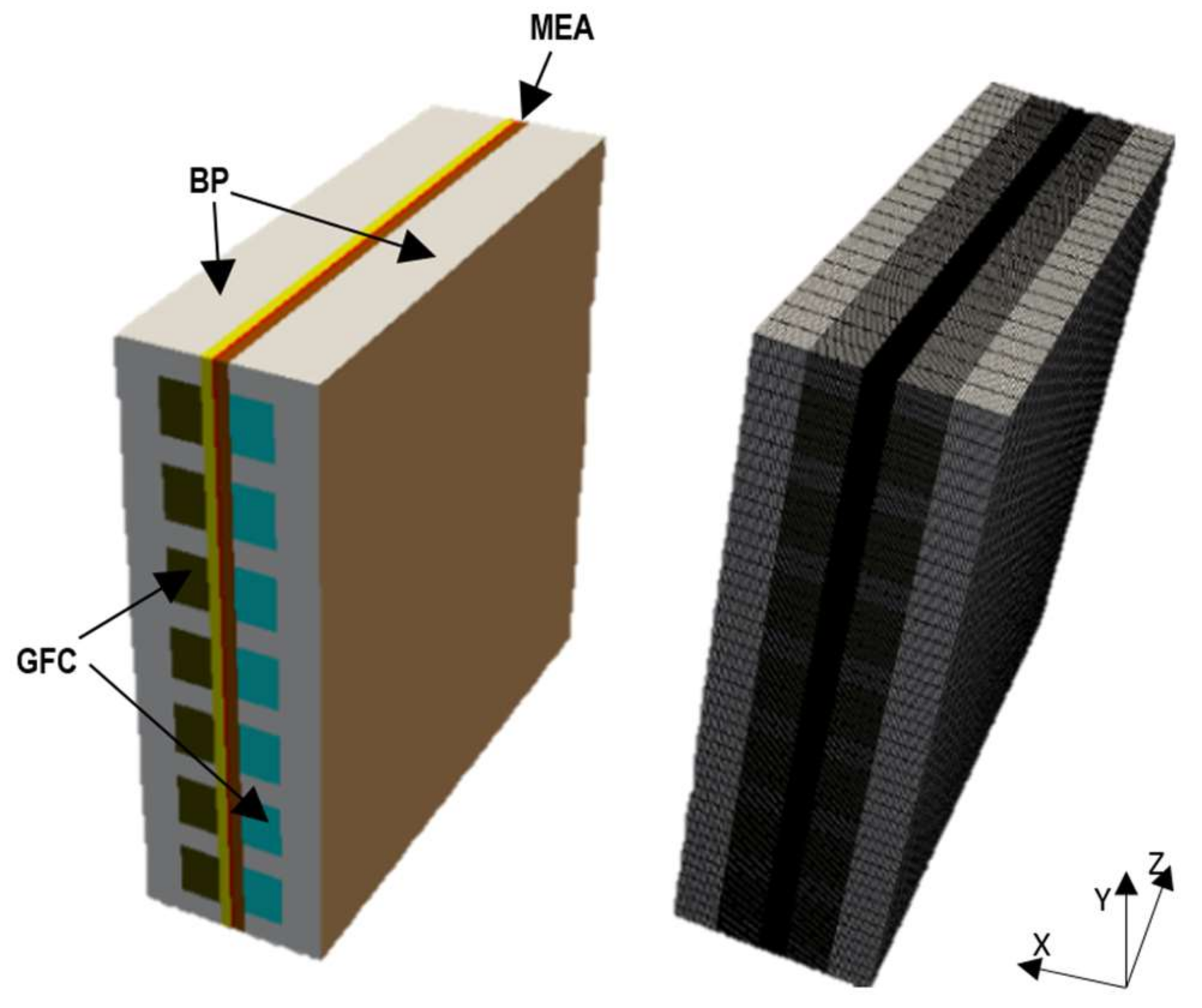
A 3D description of the cell geometry along with a mesh can be seen in Figure 1. The geometric dimensions of the components are given in Table 1. The anode and cathode electrodes, which are made up of gas diffusion layers (GDL) and catalyst layers (CL), are separated by a membrane forming the membrane electrode assembly (MEA). The MEA is inserted between two bipolar plates (BP) that accommodate the gas flow channels (GFC). The electrochemical reactions occur on the surface of the CLs where hydrogen fed into the anode GFCs reacts with oxygen that is supplied into the cathode GFCs to undergo chemical-electrical energy conversion.
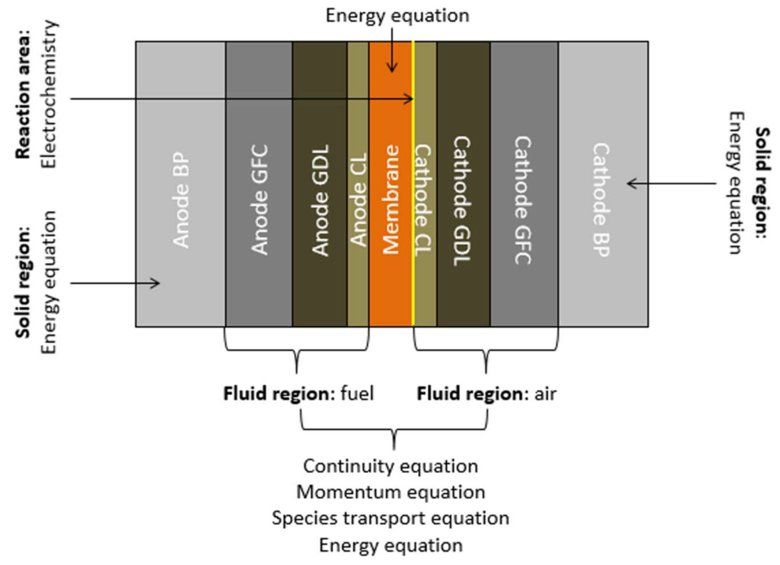
As illustrated in Figure 2, the computational domain consists of both solid and fluid regions. The solid region is comprised of the membrane and the BPs, whereas the fluid region contains the GFCs, the GDLs, and the CLs. The reactant gases and the product water are transported within the fluid region. The porous electrodes carry the heat released by the electrochemical reactions to the cooling system through the BPs. Therefore, the field variables that need to be solved in these regions are different. The solid is governed by the conservation of energy, whereas the fluid is governed by the conservations of mass, momentum, chemical species, and energy.
In the numerical model presented in this work, the conservation equations are coupled with the solution of the Nernst equation. In other words, the transport of mass, momentum, and chemical species are coupled with electrochemical reactions to create a more tractable numerical model. The energy equation solved in the solid region is coupled with the energy solutions in the fluid region.
2.2. Assumptions
Steady-state operating condition is assumed, with the gas flow considered to be laminar and incompressible due to low velocities. The individual gases and the gas mixture are considered as ideal gases. The fuel cell components are assumed to be isotropic and homogeneous. The membrane is assumed to be fully humidified and impermeable to reactant gases [26]. The electrochemical reactions are assumed to occur at the cathode electrode-membrane interface [24]. The anode’s activation and mass transport overpotentials are taken as negligible [26]. Ohmic heating in the bipolar plates is neglected due to high heat conductivity and the electrical potential distribution is taken as constant within the bipolar plates due to high electrical conductivity of the bipolar plate material [27,28]. The outer walls of the entire cell are taken as impassable to heat [24].
2.3. Governing Equations
Mass conservation:
Momentum conservation:
where the momentum source term SM, is equal to zero in the gas flow channels and to the Darcy resistance in the porous media, given by:
Chemical species conservation:
where the mass fraction of the inert species is calculated using the sum of the other species (.
Energy conservation:
where the energy source term SE, is essentially due to the heat released by the electrochemical reaction determined by:
The cell voltage:
Additional constitutive relations for linking the various physical quantities are given in Table 2.
2.4. Boundary Conditions
The boundary and initial values are given in Table 3. The inlet values for velocity, temperature, and mass fractions are given at the fluid inlets. Air and fuel inlet velocities are calculated according to [36]
The outlet pressure value is prescribed at the outlet of both the anode and the cathode gas flow channels. For all other variables, Neumann boundary conditions are applied at the fluid outlets. Impermeability conditions are specified for mass and species flow at the membrane-fluid interfaces. Impermeability, no-slip, and no-flux boundary conditions are applied at all the internal surfaces within the modelling domain. A temperature of zero-gradient is applied at all the external surfaces.
3. Numerical Implementation
3.1. Computational Procedure
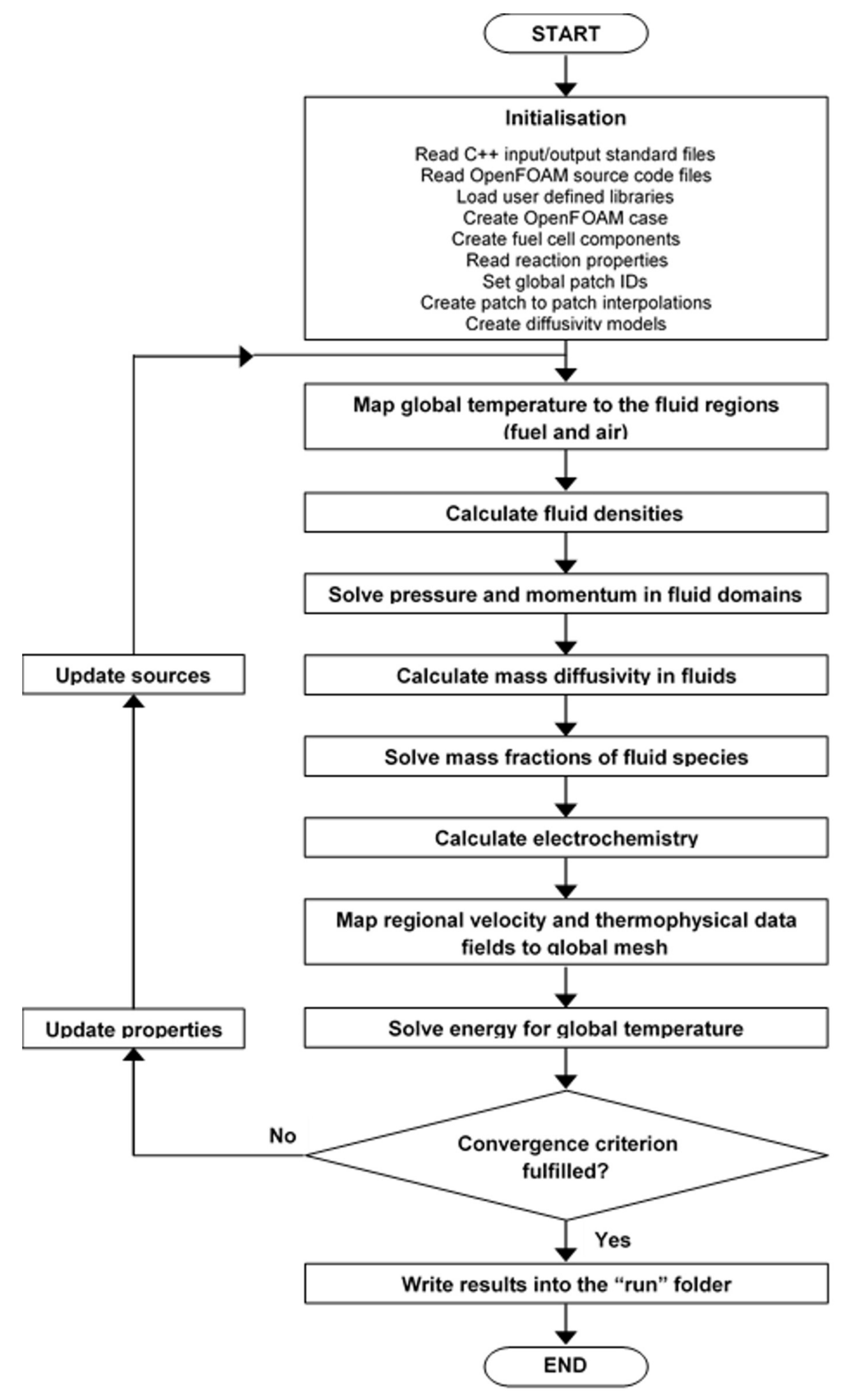
The flow diagram of the solution procedure is shown in Figure 3. The initialization phase is followed by an iteration loop where several calculations are repeated until convergence. For the potentiostatic (i.e., current density calculation) run, the cell voltage is fixed whereas for the galvanostatic (i.e., voltage calculation) run, it is adjusted until the computed mean current density is equal or very close to its initial value.
3.2. Toolbox Structure
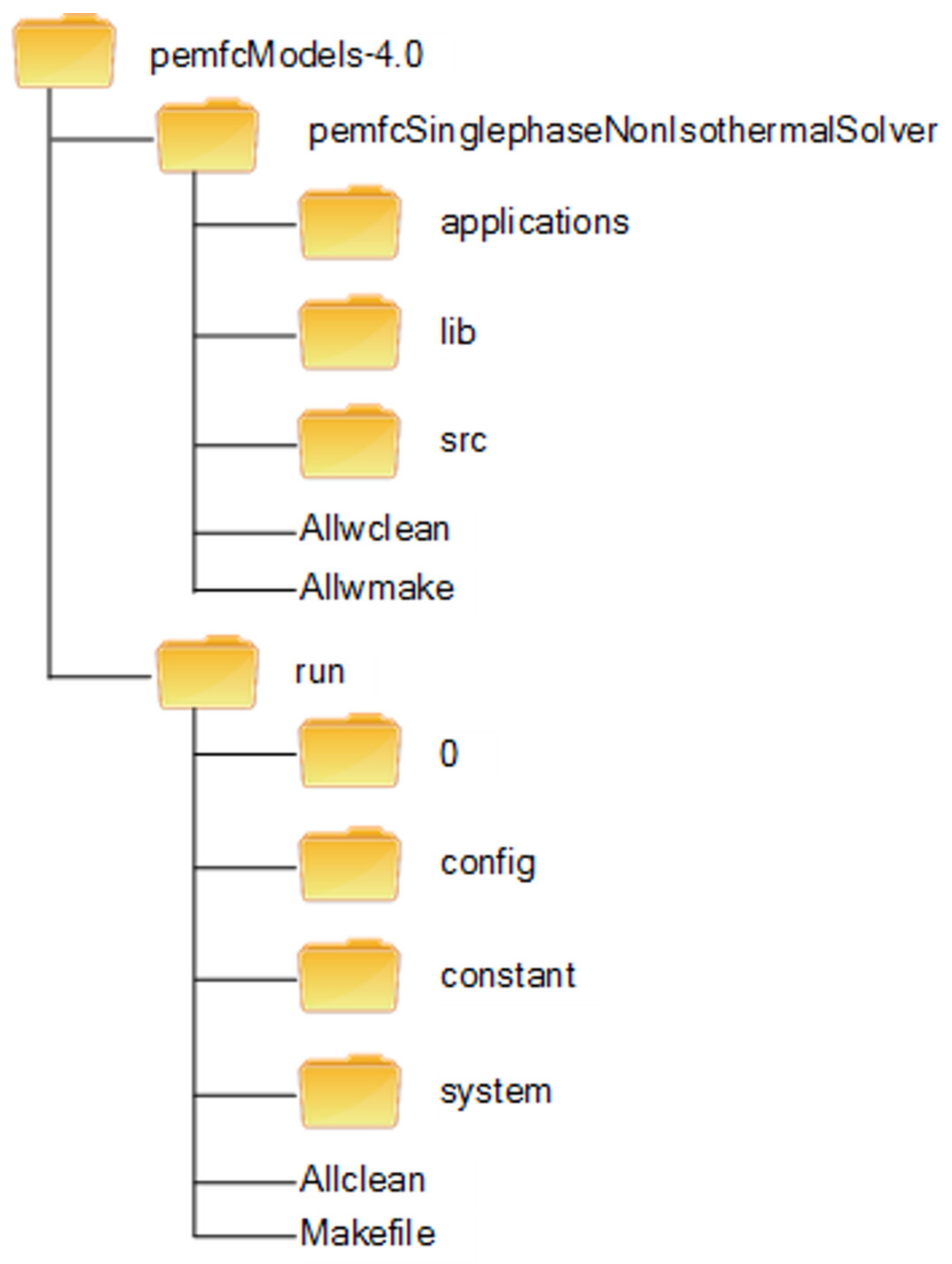
The present toolbox follows the same structure and organization as OpenFOAM, as depicted in Figure 4. OpenFOAM is essentially a C++ library with its components falling into two main categories: solvers and utilities. Users can customize any existing components to suit their needs although this requires a good understanding of the software structure, as well as the programming techniques involved. One shortcoming of the OpenFOAM software package is that it has no PEM fuel cell module. Thus, the toolbox developed here provides remediation for this situation. It has two major components: pemfcSinglephaseNonIsothermalSolver and run.
3.2.1. PemfcSinglephaseNonIsothermalSolver
The pemfcSinglephaseNonIsothermalSolver folder contains the source code for the solver and libraries. A pemfcSinglephaseNonIsothermalSolver.c file that contains the main loop of the program is stored in the applications sub-folder. The lib sub-folder is where all necessary libraries are stored and compiled. These include, amongst other things, classes for multicomponent gas diffusivities, geometry, and mesh manipulation. The src sub-folder stores various program files containing specific instructions for the initialization phase and algorithms for solving field variables in the main loop. The individual solvers and other algorithmic controls and tolerances for these field variables are defined in the fvSolution files present in the system sub-folder of the run folder.
3.2.2. Run
The run folder contains the constructed simulation case. An OpenFOAM case folder usually contains three main sub-folders that store several files necessary to running OpenFOAM applications. The 0 sub-folder is a time sub-folder that stores the initial field data. In OpenFOAM, the time sub-folders store all the field data at various times; the name of each sub-folder corresponds to the time at which the simulation data were written. The data for the geometry construction and mesh creation are stored in the config sub-folder. The constant sub-folder contains a sub-sub-folder called polyMesh in which the mesh information and boundary condition files are stored, along with the physical property file. The files for the solution control, scheme and solvers are stored in the system sub-folder.
4. Model Verification
4.1. Mesh Independence Study
To prove that the solution is independent from the mesh, a mesh independence study was conducted. This required refining the case study mesh twice by adding an extra 20% and 40% of the cells in every direction. Simulations at the case study conditions were then run with these refined meshes in order to compare the solutions for the temperature field. The numerical results, shown in Table 7, showed that the maximum change of temperature solution is 0.03% for the compared meshes. This is evidence of the independence of the solution from the grid.
4.2. Comparison with Literature Model Results and Experimental Data
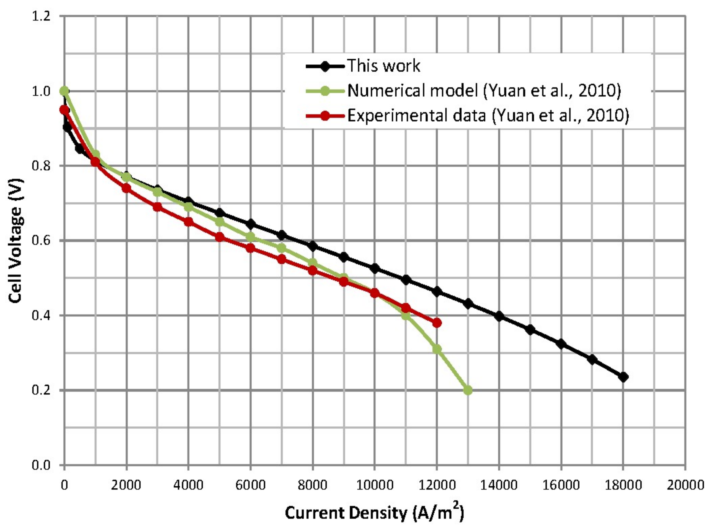
The cell voltage drop per current density, also known as polarization curve, is plotted in Figure 5. Since the present single-phase flow model has been run with some of the parameters and properties taken from the multiphase flow model introduced by Yuan et al. [38] (as given in Table 8), the results are therefore compared to the numerical model results and experimental data from Yuan et al. [38]. This also required adjusting other parameters such as the charge transfer coefficient and the reference exchange current density to achieve a good agreement between the models (see Table 8). A direct comparison is problematic given some differences in the modelling approaches, as well as cell geometric dimensions and operating condition parameters and properties (see Table 8). But the polarization curves nonetheless follow similar trends as seen in Figure 5, which confirms the trend in cell voltage drop obtained with the developed OpenFOAM model. However, this work does not account for liquid water effects in the fuel cell, which would have resulted in further potential drop, as accounted for in the multiphase flow model in [38]. Furthermore, the difference between the three curves at high current densities is due to, in addition to other factors, the complex conjunction of the effects of the inlet flow rates, the cell design details and properties (e.g., number of gas flow channels in each electrode, electrode porosity, material properties, etc., see Table 8), and the concentration overpotential. In fact, the result indicates that the impact of the chosen concentration constant on the concentration overpotential is very significant. Hence, optimization of this value would play a key role in shaping the cell I-V curve since the curvature in the high current densities zone is determined by the changes in the concentration overpotential.
5. Case Study Results and Discussion
The results are post-processed and visualized using ParaView, which is an open source visualization software used for postprocessing in OpenFOAM through the paraFoam utility, supplied with OpenFOAM.
The velocity profiles along the gas flow channels for the fuel and air are displayed in Figure 6a,b, respectively. These are consistent with those seen in fully-developed laminar flow. The highest velocity appears at the center lines of the channels and the lowest velocity is seen at the walls.
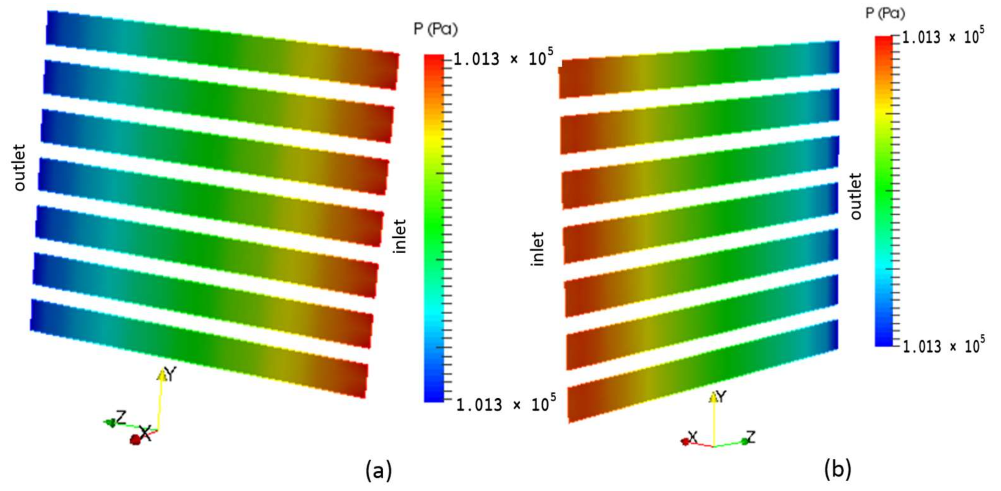
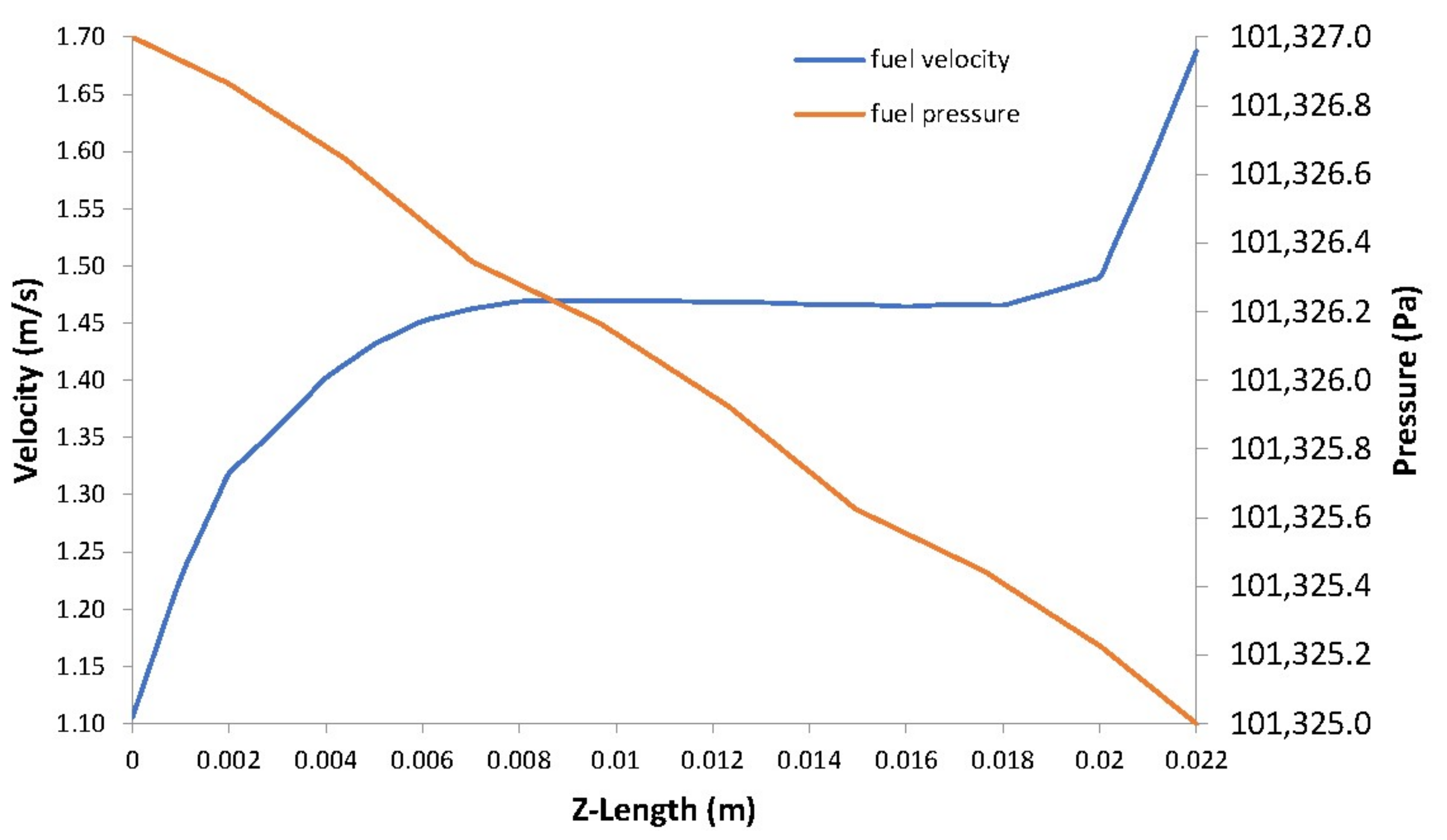
The pressure in the fuel and air side gas flow channels are illustrated in Figure 7a,b, respectively. A pressure drop occurs at the outlets of the channels as the velocity increases in these areas as shown in Figure 8 and Figure 9.
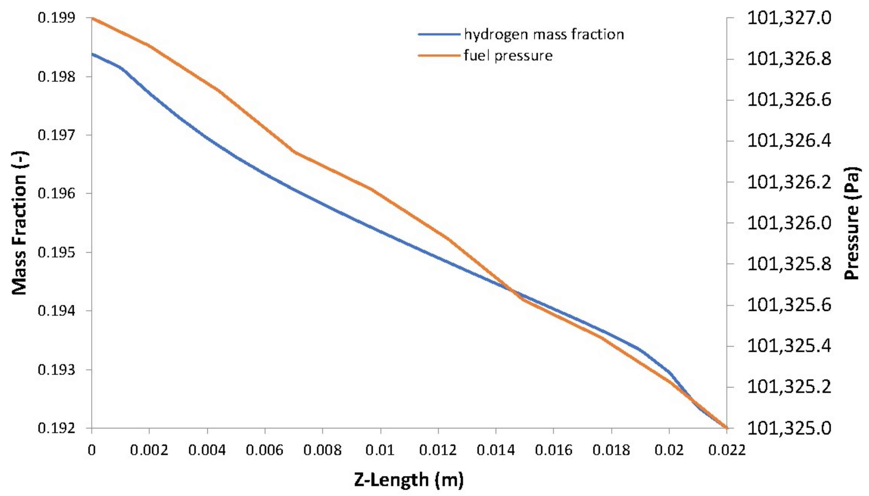
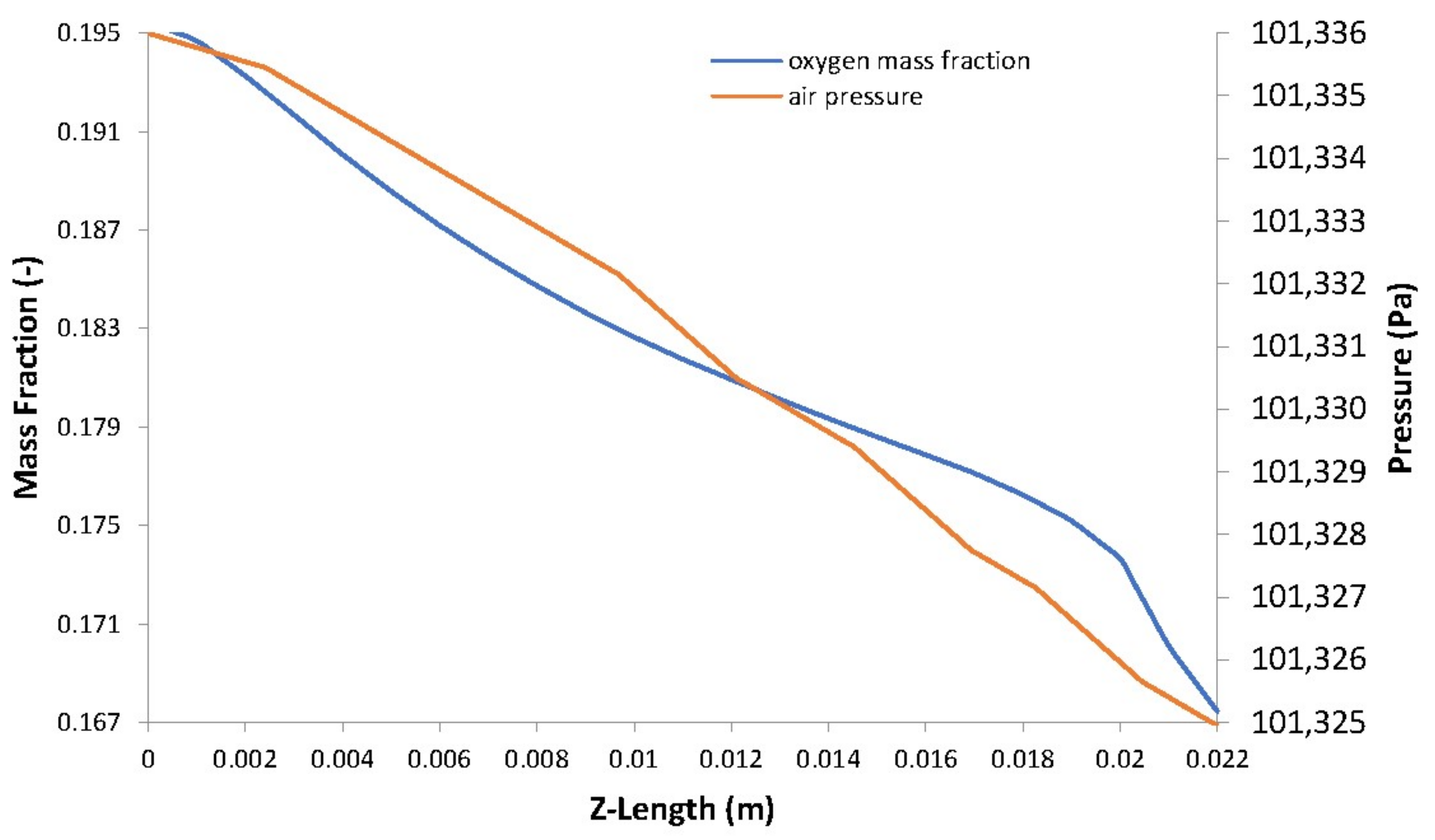
The distribution of hydrogen and oxygen mass fractions are shown in Figure 10a,b, respectively. The consumption of the reactant gases by the electrochemical reaction leads to a decrease in their mass fractions going from inlet to outlet and from the GFCs to the CLs. There is a direct proportionality between the concentration of reactant gases in the electrodes and the pressure (see Figure 11 and Figure 12).
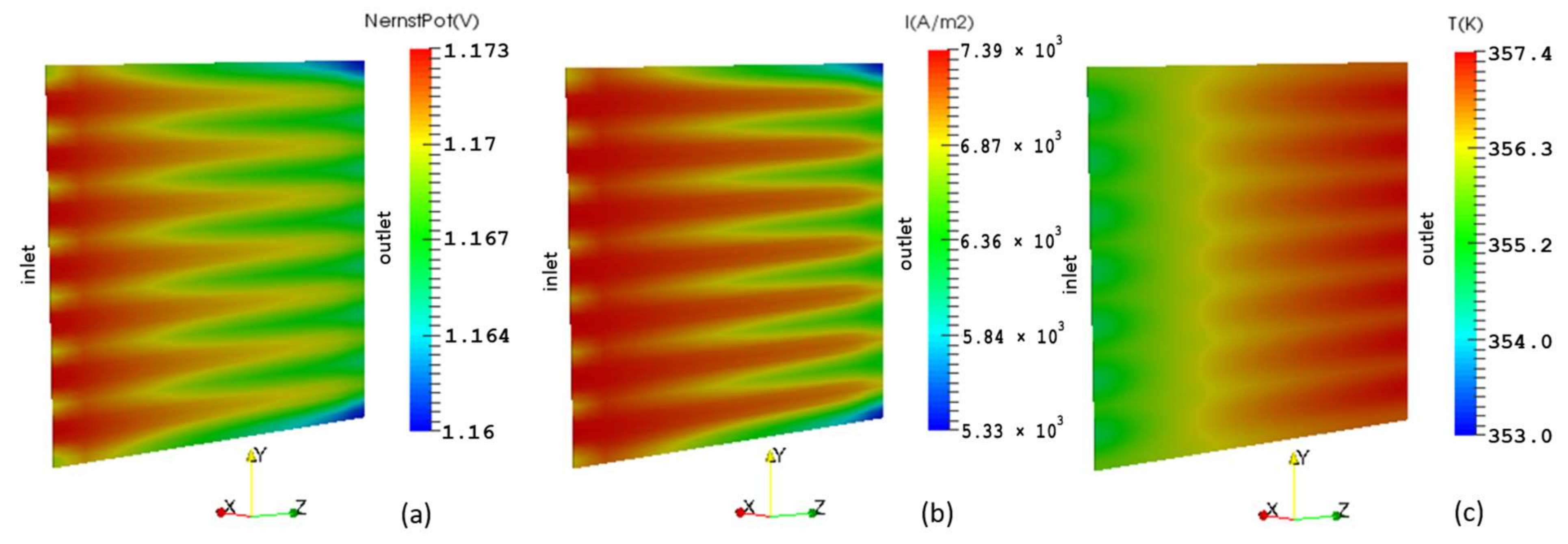
The distribution of Nernst potential is illustrated in Figure 13a. The combined effects of hydrogen depletion in the anode and water vapor production in the cathode cause the Nernst potential to decline from inlet to outlet. Consequently, the observed local current density as shown in Figure 13b, also decreases in the flow direction. The current density sharply decreases towards the corner edges of the cell outlet where there is no active surface. The distribution of the local temperature is displayed in Figure 13c. The non-uniform nature of the temperature field is due to thermal inactivity at the ribs. This reduces the heat released by the electrochemical reaction in these areas, which in turn lowers the current densities due to reduced mass transfer.
6. Conclusions and Outlook
An open-source code toolbox capable of accurately predicting the distribution of the major physical quantities that are transported within a PEM fuel cell has been created using OpenFOAM. The toolbox can be used to rapidly gain important insights into the cell working processes that are essential for design optimization. It consists of a main program, relevant library classes, and a constructed simulation case for a co-flow galvanostatic run.
The base case results for the distribution of velocity, pressure, chemical species, Nernst potential, current density, and temperature are as expected. The results of a mesh independence investigation revealed that the solution is independent from the grid. The plotted cell polarization curve was compared to the available experimental data and numerical model results taken from the literature, though a direct comparison seems difficult because of the differences in the modelling approaches, as well as cell geometric dimensions and operating condition parameters and properties. The obtained simulation data can provide crucial information about the major transport processes that take place within a PEM fuel cell.
The model that has been created can, by no means, be considered complete. There are still some improvements that can be made in the context of the present study. Liquid water transport has not been considered, and so far, the transport phenomena inside the membrane (e.g., dissolved water transport) have been simplified. Also, for the sake of simplicity, and to facilitate the numerical implementation, the electrochemical reaction has been assumed to take place at a single interface between the cathode catalyst layer and the membrane.
The present tool can provide a foundation for further development that is not always feasible with commercial code. The source code is available at http://dx.doi.org/10.17632/3gz7pxznzn.1. Future work may include a multiphase flow extension, and or improved catalyst and membrane models, as well as performing a detailed sensitivity analysis for a deeper understanding of the modelling choices. Moreover, experimental test of the fuel cell used in the case study will be conducted in the future to validate the results obtained here from CFD simulation.
Author Contributions
Conceptualization, J.-P.K.; Methodology, J.-P.K. and X.Z.; Software, J.-P.K.; Validation, J.-P.K., X.Z. and Y.Y.; Formal Analysis, J.-P.K. and S.A.; Investigation, J.-P.K.; Resources, X.Z.; Data Curation, J.-P.K.; Writing-Original Draft Preparation, J.-P.K.; Writing-Review & Editing, X.Z. and S.A.; Visualization, J.-P.K.; Supervision, X.Z. and Y.Y.; Project Administration, J.-P.K. and S.A.; Funding Acquisition, X.Z.
Funding
This research was funded by [UK Engineering and Physical Sciences Research Council] grant number [EP/G037345/1 and EP/L016362/1] and [Ningbo Science and Technology Bureau Technology Innovation Team] grant number [No. 2016B10010].
Acknowledgments
The authors acknowledge the financial and administrative support from the International Doctoral Innovation Centre, Ningbo Education Bureau, Ningbo Science and Technology Bureau, and the University of Nottingham. This work was also supported by the Faculty of Science and Engineering at University of Nottingham Ningbo China (SRG code 01.03.05.04.2015.02.001), Ningbo Natural Science Foundation Program (project code 2013A610107), Zhejiang Natural Science Foundation (project code LY18E060004).
Conflicts of Interest
The authors declare no conflict of interest. The founding bodies had no role in the design of the study, collection, analyses, interpretation of data; writing of the manuscript, and in the decision to publish the results.
List of Symbols
| A | area, m2 |
| C | concentration, mol m−3 |
| cp | specific heat capacity, J kg−1 K−1 |
| d | diameter, m |
| D | diffusivity, m2 s−1 |
| E | potential, V |
| F | Faraday’s constant, 96,485 C mol−1 e− |
| ΔG | Gibbs free energy, kJ mol−1 |
| H | latent heat, J kg−1 |
| ΔH | enthalpy of formation, J mol−1 |
| I | current density, A m−2 |
| I0 | exchange current density, A m−2 |
| k | thermal conductivity, W m−1 K−1 |
| K | permeability, m2 |
| M | molar mass, kg kmol−1 |
| ni | number of electron of species i |
| p | pressure, Pa |
| R | universal gas constant, 8.314 J mol−1 K−1 |
| RΩ | area specific resistance, Ω m2 |
| ∆S | entropy of formation, J mol−1 K−1 |
| T | temperature, K |
| velocity vector, m s−1 | |
| v | diffusion volume, m3 |
| V | voltage, V |
| y | mass fraction |
| x | mole fraction |
| z | number of electron transferred |
| Greek letters | |
| α | charge transfer coefficient |
| δ | thickness, m |
| ε | porosity |
| η | overpotential, V |
| μ | dynamic viscosity, Pa s |
| ξ | stoichiometric ratio |
| ρ | density, kg m−3 |
| σe | electrical conductivity, S m−1 |
| σi | ionic conductivity, S m−1 |
| τ | tortuosity |
| Subscripts and superscripts | |
| act | activation |
| c | cathode |
| ch | channel |
| con | concentration |
| E | energy |
| eff | effective |
| H2 | hydrogen |
| H2O | water |
| i | species i |
| j | species j |
| knud | Knudsen |
| L | limiting |
| M | momentum |
| MEA | membrane electrode assembly |
| MEM | membrane |
| mix | mixture |
| N2 | nitrogen |
| O2 | oxygen |
| ohm | ohmic |
| p | pore |
| ref | reference |
| sat | saturation |
| WV | water vapor |
References
- Kone, J.P.; Zhang, X.; Yan, Y.; Hu, G.; Ahmadi, G. Three-dimensional multiphase flow computational fluid dynamics models for proton exchange membrane fuel cell: A theoretical development. J. Comput. Multiph. Flows 2017, 9, 3–25. [Google Scholar] [CrossRef]
- Wu, H.W. A review of recent development: Transport and performance modeling of pem fuel cells. Appl. Energy 2016, 165, 81–106. [Google Scholar] [CrossRef]
- Ferreira, R.B.; Falcao, D.S.; Oliveira, V.B.; Pinto, A. Numerical simulations of two-phase flow in proton exchange membrane fuel cells using the volume of fluid method—A review. J. Power Sources 2015, 277, 329–342. [Google Scholar] [CrossRef]
- Weber, A.Z.; Borup, R.L.; Darling, R.M.; Das, P.K.; Dursch, T.J.; Gu, W.B.; Harvey, D.; Kusoglu, A.; Litster, S.; Mench, M.M.; et al. A critical review of modeling transport phenomena in polymer-electrolyte fuel cells. J. Electrochem. Soc. 2014, 161, F1254–F1299. [Google Scholar] [CrossRef]
- Wilberforce, T.; El-Hassan, Z.; Khatib, F.N.; Al Makky, A.; Mooney, J.; Barouaji, A.; Carton, J.G.; Olabi, A.G. Development of bi-polar plate design of pem fuel cell using cfd techniques. Int. J. Hydrogen Energy 2017, 42, 25663–25685. [Google Scholar] [CrossRef]
- Zhao, D.D.; Dou, M.F.; Zhou, D.M.; Gao, F. Study of the modeling parameter effects on the polarization characteristics of the pem fuel cell. Int. J. Hydrogen Energy 2016, 41, 22316–22327. [Google Scholar] [CrossRef]
- Laoun, B.; Naceur, M.W.; Khellaf, A.; Kannan, A.M. Global sensitivity analysis of proton exchange membrane fuel cell model. Int. J. Hydrogen Energy 2016, 41, 9521–9528. [Google Scholar] [CrossRef]
- Khazaee, I.; Sabadbafan, H. Effect of humidity content and direction of the flow of reactant gases on water management in the 4-serpentine and 1-serpentine flow channel in a pem (proton exchange membrane) fuel cell. Energy 2016, 101, 252–265. [Google Scholar] [CrossRef]
- Xing, L.; Cai, Q.; Xu, C.X.; Liu, C.B.; Scott, K.; Yan, Y.S. Numerical study of the effect of relative humidity and stoichiometric flow ratio on pem (proton exchange membrane) fuel cell performance with various channel lengths: An anode partial flooding modelling. Energy 2016, 106, 631–645. [Google Scholar] [CrossRef]
- Sezgin, B.; Caglayan, D.G.; Devrim, Y.; Steenberg, T.; Eroglu, I. Modeling and sensitivity analysis of high temperature pem fuel cells by using comsol multiphysics. Int. J. Hydrogen Energy 2016, 41, 10001–10009. [Google Scholar] [CrossRef]
- Ozen, D.N.; Timurkutluk, B.; Altinisik, K. Effects of operation temperature and reactant gas humidity levels on performance of pem fuel cells. Renew. Sustain. Energy Rev. 2016, 59, 1298–1306. [Google Scholar] [CrossRef]
- Osanloo, B.; Mohammadi-Ahmar, A.; Solati, A. A numerical analysis on the effect of different architectures of membrane, cl and gdl layers on the power and reactant transportation in the square tubular pemfc. Int. J. Hydrogen Energy 2016, 41, 10844–10853. [Google Scholar] [CrossRef]
- Khazaee, I.; Sabadbafan, H. Numerical study of changing the geometry of the flow field of a pem fuel cell. Heat Mass Transf. 2016, 52, 993–1003. [Google Scholar] [CrossRef]
- Velisala, V.; Srinivasulu, G.N. Numerical simulation and experimental comparison of single, double and triple serpentine flow channel configuration on performance of a pem fuel cell. Arab. J. Sci. Eng. 2018, 43, 1225–1234. [Google Scholar] [CrossRef]
- Wang, Y.L.; Wang, S.X.; Wang, G.Z.; Yue, L.K. Numerical study of a new cathode flow-field design with a sub-channel for a parallel flow-field polymer electrolyte membrane fuel cell. Int. J. Hydrogen Energy 2018, 43, 2359–2368. [Google Scholar] [CrossRef]
- Ashrafi, M.; Shams, M. The effects of flow-field orientation on water management in pem fuel cells with serpentine channels. Appl. Energy 2017, 208, 1083–1096. [Google Scholar] [CrossRef]
- Zehtabiyan-Rezaie, N.; Arefian, A.; Kermani, M.J.; Noughabi, A.K.; Abdollahzadeh, M. Effect of flow field with converging and diverging channels on proton exchange membrane fuel cell performance. Energy Convers. Manag. 2017, 152, 31–44. [Google Scholar] [CrossRef]
- Barreras, F.; Lozano, A.; Valino, L.; Mustafa, R.; Marin, C. Fluid dynamics performance of different bipolar plates—Part I. Velocity and pressure fields. J. Power Sources 2008, 175, 841–850. [Google Scholar] [CrossRef]
- Lozano, A.; Valino, L.; Barreras, F.; Mustata, R. Fluid dynamics performance of different bipolar plates—Part II. Flow through the diffusion layer. J. Power Sources 2008, 179, 711–722. [Google Scholar] [CrossRef]
- Mustata, R.; Valino, L.; Barreras, F.; Gil, M.I.; Lozano, A. Study of the distribution of air flow in a proton exchange membrane fuel cell stack. J. Power Sources 2009, 192, 185–189. [Google Scholar] [CrossRef]
- Valino, L.; Mustata, R.; Gil, M.I.; Martin, J. Effect of the relative position of oxygen-hydrogen plate channels and inlets on a pemfc. Int. J. Hydrogen Energy 2010, 35, 11425–11436. [Google Scholar] [CrossRef]
- Imbrioscia, G.M.; Fasoli, H.J. Simulation and study of proposed modifications over straight-parallel flow field design. Int. J. Hydrogen Energy 2014, 39, 8861–8867. [Google Scholar] [CrossRef]
- Valino, L.; Mustata, R.; Duenas, L. Consistent modeling of a single pem fuel cell using onsager’s principle. Int. J. Hydrogen Energy 2014, 39, 4030–4036. [Google Scholar] [CrossRef]
- Beale, S.B.; Choi, H.-W.; Pharoah, J.G.; Roth, H.K.; Jasak, H.; Jeon, D.H. Open-source computational model of a solid oxide fuel cell. Comput. Phys. Commun. 2016, 200, 15–26. [Google Scholar] [CrossRef]
- Kone, J.P.; Zhang, X.; Yan, Y.; Hu, G.; Ahmadi, G. CFD Modeling and Simulation of Pem Fuel Cell Using Openfoam. In Proceedings of the Applied Energy Symposium and Forum, REM2017: Renewable Energy Integration with Mini/Microgrid, Tianjin, China, 18–20 October 2017. [Google Scholar]
- Barbir, F. Pem Fuel Cells: Theory and Practice; Elsevier Academic: Amsterdam, The Netherlands; London, UK, 2005; p. 15. 433p. [Google Scholar]
- Sivertsen, B.R.; Djilali, N. Cfd-based modelling of proton exchange membrane fuel cells. J. Power Sources 2005, 141, 65–78. [Google Scholar] [CrossRef]
- Ju, H.; Meng, H.; Wang, C.Y. A single-phase, non-isothermal model for pem fuel cells. Int. J. Heat Mass Transf. 2005, 48, 1303–1315. [Google Scholar] [CrossRef]
- Poling, B.E.; Prausnitz, J.M.; O’Connell, J.P. The Properties of Gases and Liquids, 5th ed.; McGraw-Hill: New York, NY, USA, 2000. [Google Scholar]
- Fairbanks, D.F.; Wilke, C.R. Diffusion coefficients in multicomponent gas mixtures. Ind. Eng. Chem. 1950, 42, 471–475. [Google Scholar] [CrossRef]
- Welty, J.R.; Wicks, C.E.; Wilson, R.E.; Rorrer, G.L. Fundamentals of Momentum, Heat, and Mass Transfer, 5th ed.; Wiley: Hoboken, NJ, USA, 2008. [Google Scholar]
- Geankoplis, C.J. Transport Processes and Unit Operations, 3rd ed.; Prentice-Hall: Upper Saddle River, NJ, USA, 1993. [Google Scholar]
- Springer, T.E.; Zawodzinski, T.A.; Gottesfeld, S. Polymer electrolyte fuel-cell model. J. Electrochem. Soc. 1991, 138, 2334–2342. [Google Scholar] [CrossRef]
- O’Hayre, R.P.; Cha, S.-W.; Colella, W.; Prinz, F.B. Fuel Cell Fundamentals; John Wiley & Sons: Hoboken, NJ, USA, 2006. [Google Scholar]
- Wang, Y.; Chen, K.S.; Cho, S.C. Pem Fuel Cells:hermal and Water Management Fundamentals; Momentum Press: New York, NY, USA, 2013. [Google Scholar]
- Liu, Z. Fuel Cell Performance; Nova Science Publishers: New York, NY, USA, 2012; p. 10. 284p. [Google Scholar]
- Chang, R.; Goldsby, K.A. General Chemistry: The Essential Concepts; McGraw-Hill: New York, NY, USA, 2014. [Google Scholar]
- Yuan, W.; Tang, Y.; Pan, M.Q.; Li, Z.T.; Tang, B. Model prediction of effects of operating parameters on proton exchange membrane fuel cell performance. Renew. Energy 2010, 35, 656–666. [Google Scholar] [CrossRef]
- Todd, B.; Young, J.B. Thermodynamic and transport properties of gases for use in solid oxide fuel cell modelling. J. Power Sources 2002, 110, 186–200. [Google Scholar] [CrossRef]
- Yaws, C.L. Yaws’ Critical Property Data for Chemical Engineers and Chemists; Knovel: New York, NY, USA, 2012. [Google Scholar]
- Parthasarathy, A.; Dave, B.; Srinivasan, S.; Appleby, A.J.; Martin, C.R. The platinum microelectrode nafion interface—An electrochemical impedance spectroscopic analysis of oxygen reduction kinetics and nafion characteristics. J. Electrochem. Soc. 1992, 139, 1634–1641. [Google Scholar] [CrossRef]
- Yaws, C.L. Yaws’ Handbook of Thermodynamic Properties for Hydrocarbons and Chemicals; Knovel: New York, NY, USA, 2009. [Google Scholar]
- Fuller, E.N.; Schettle, P.D.; Giddings, J.C. A new method for prediction of binary gas-phase diffusion coeffecients. Ind. Eng. Chem. 1966, 58, 19–27. [Google Scholar]
- Fuller, E.N.; Ensley, K.; Giddings, J.C. Diffusion of halogenated hydrocarbons in helium. Effect of structure on collision cross sections. J. Phys. Chem. 1969, 73, 3679–3685. [Google Scholar] [CrossRef]
Figure 1.
Geometry and mesh of a single cell proton exchange membrane (PEM) fuel cell.

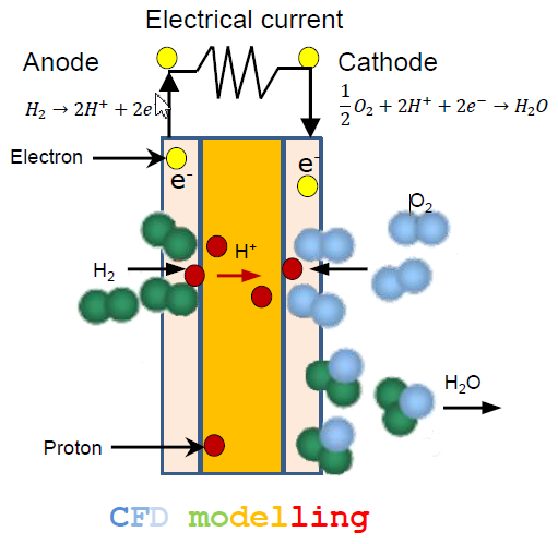
Figure 2.
Transport processes in a PEM fuel cell.

Figure 3.
Flow diagram of the solution procedure.

Figure 4.
File structure of the toolbox.

Figure 5.
Cell polarization curve compared to the literature model and experimental data.

Figure 6.
Velocity profiles along the gas flow channels: (a) Fuel; (b) Air.
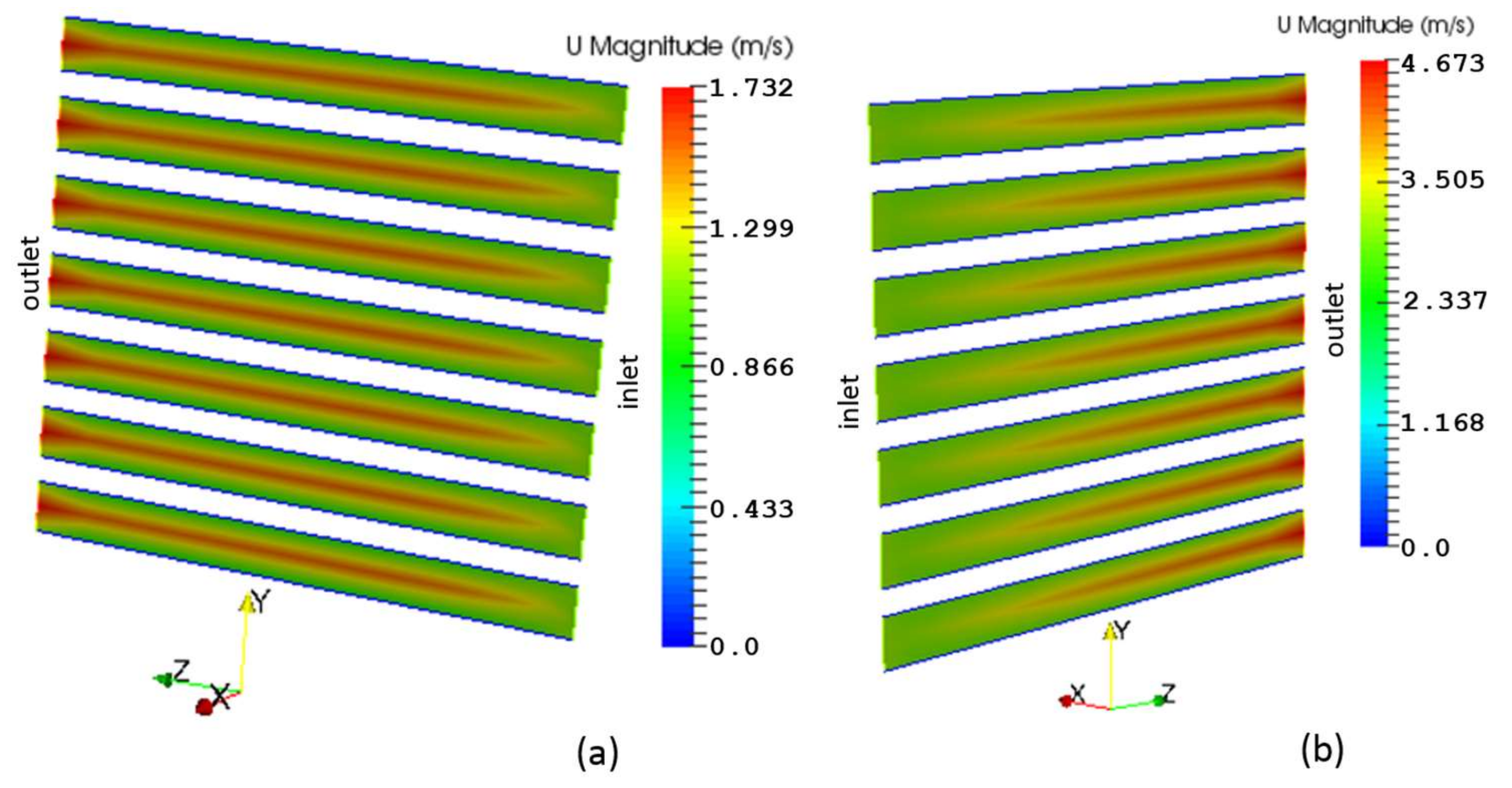
Figure 7.
Pressure distribution in the gas flow channels: (a) Fuel; (b) Air.

Figure 8.
Fuel velocity vs. fuel pressure.

Figure 9.
Air velocity vs. air pressure.
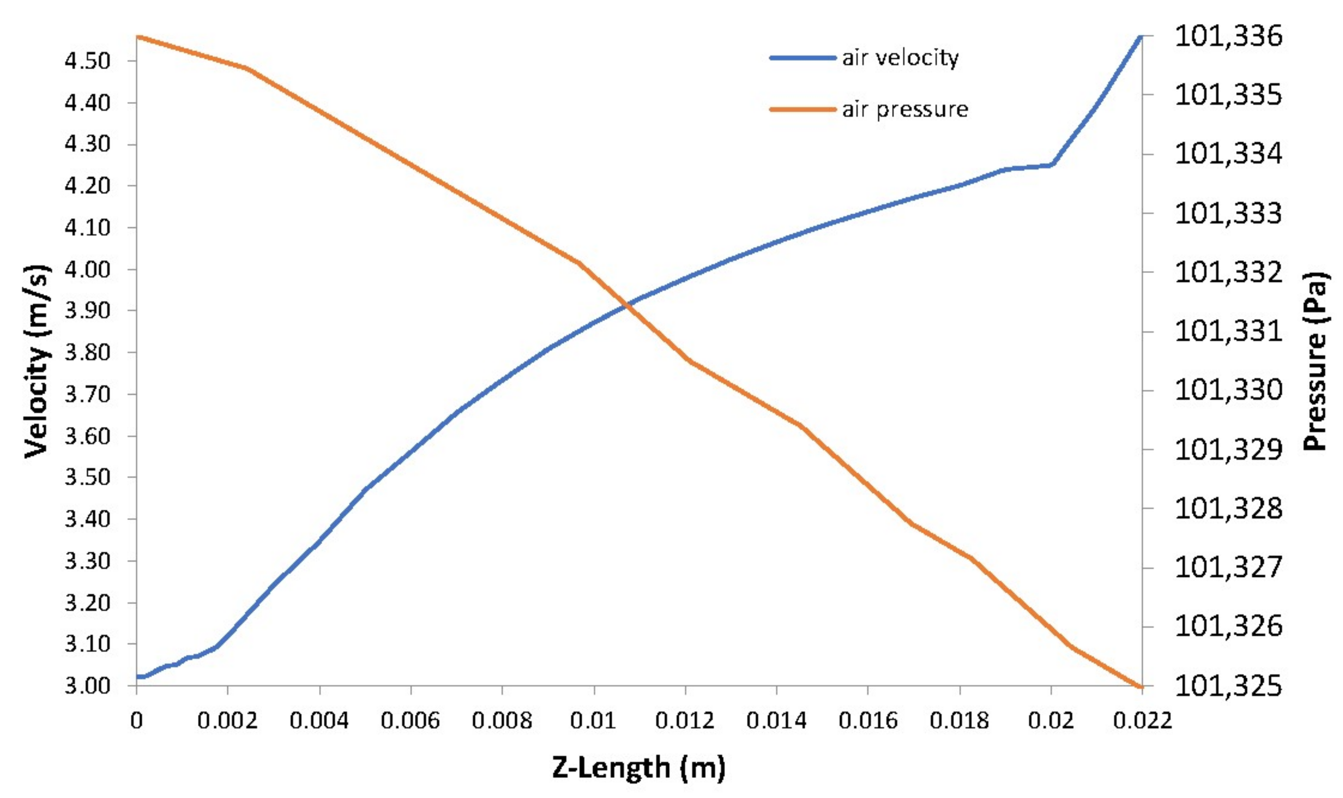
Figure 10.
Species mass fraction distribution: (a) Hydrogen; (b) Oxygen.
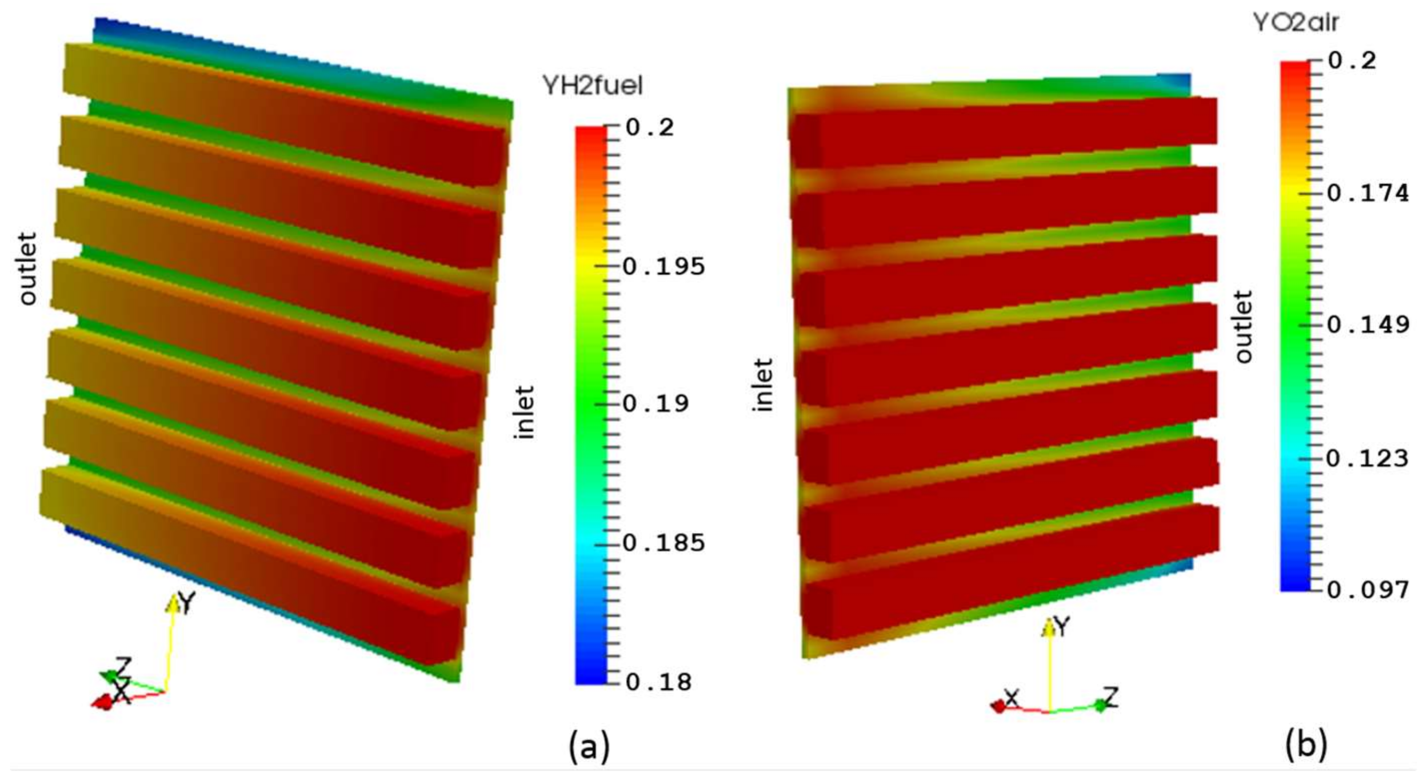
Figure 11.
Hydrogen mass fraction vs. fuel pressure.

Figure 12.
Oxygen mass fraction vs. air pressure.

Figure 13.
Membrane cathode interface showing the distribution of: (a) Nernst potential; (b) Local current density; (c) Temperature.
Figure 13.
Membrane cathode interface showing the distribution of: (a) Nernst potential; (b) Local current density; (c) Temperature.


Table 1.
The cell geometric dimensions [25].
Table 1.
The cell geometric dimensions [25].
| BP | GFC | GDL | CL | Membrane | |
|---|---|---|---|---|---|
| x-width (mm) | 3 | 1.5 | 0.41 | 0.0037 | 0.127 |
| y-height (mm) | 22 | 2 | 22 | 22 | 22 |
| z-length (mm) | 22 | 22 | 22 | 22 | 22 |
Table 2.
Constitutive equations.
| Description | Symbol | Expression | Source |
|---|---|---|---|
| Gas density | ρ | - | |
| Mole fraction | xi | - | |
| Specific heat capacity | cp | - | |
| Thermal conductivity | k | [29] | |
| Diffusivity of gas species i | Di-mix | [30] | |
| Effective global diffusivity | [31] | ||
| Effective species diffusivity | [31] | ||
| Effective Knudsen diffusivity | [31] | ||
| Knudsen diffusion coefficient | Di-Knud | [32] | |
| Nernst potential | ENernst | - | |
| Area specific resistance | RΩ | [33] | |
| Membrane ionic conductivity | σi | [33] | |
| Membrane water content | λ | [33] | |
| Water vapor activity | a | [33] | |
| Saturation pressure | [33] | ||
| Activation overpotential | ηact | [26] | |
| Ohmic overpotential | ηohm | [26] | |
| Concentration overpotential | ηcon | [34] | |
| Concentration constant | c | [34] | |
| Limiting current density | IL | [26] | |
| Cathode exchange current density | I0,C | [35] | |
| Species mass flux | [26] |
Table 3.
Boundary and initial values.
| Equations | Anode Inlet | Anode Outlet | Cathode Inlet | Cathode Outlet | Walls |
|---|---|---|---|---|---|
| Momentum | Ufuel = 1.1055 m s−1 | pfuel = 101,325 Pa | Uair = 3.082 m s−1 | pair = 101,325 Pa | U = 0 |
| Species transport | . | ||||
| Energy | T = 353 K | T = 353 K |
Table 4.
Physical constants and properties at 353 K.
| Parameter or Property | Symbol | Value | Unit | Source |
|---|---|---|---|---|
| Density of air | ρair | 0.914 | kg m−3 | Calculated [37] |
| Density of fuel | ρfuel | 0.2404 | kg m−3 | Calculated [37] |
| Density of membrane | ρMEM | 1980 | kg m−3 | [38] |
| Density of BP | ρBP | 1880 | kg m−3 | [38] |
| Isobaric heat capacity of air | cp,air | 1108.85 | J kg−1 K−1 | Calculated [39] |
| Isobaric heat capacity of fuel | cp,fuel | 2062.74 | J kg−1 K−1 | Calculated [39] |
| Isobaric heat capacity of GDL | cp,GDL | 710 | J kg−1 K−1 | [38] |
| Isobaric heat capacity of CL | cp,CL | 710 | J kg−1 K−1 | [38] |
| Isobaric heat capacity of membrane | cp,MEM | 2000 | J kg−1 K−1 | [38] |
| Isobaric heat capacity of BP | cp,BP | 875 | J kg−1 K−1 | [38] |
| Thermal conductivity of air | kair | 0.02867 | W m−1 K−1 | Calculated [29,39] |
| Thermal conductivity of fuel | kfuel | 0.08396 | W m−1 K−1 | Calculated [29,39] |
| Thermal conductivity of GDL | kGDL | 1.6 | W m−1 K−1 | [38] |
| Thermal conductivity of CL | kCL | 8 | W m−1 K−1 | [38] |
| Thermal conductivity of membrane | kMEM | 0.67 | W m−1 K−1 | [38] |
| Thermal conductivity of BP | kBP | 10.7 | W m−1 K−1 | [38] |
| Electronic conductivity of GDL | σe,GDL | 5000 | S m−1 | [38] |
| Electronic conductivity of CL | σe,CL | 1000 | S m−1 | [38] |
| Electronic conductivity of BP | σe,BP | 8.3 × 10⁴ | S m−1 | [38] |
| Dynamic viscosity of air | μair | 1.5158 × 10⁻⁵ | Pa s | Calculated [29,39,40] |
| Dynamic viscosity of fuel | μfuel | 1.5 × 10⁻⁵ | Pa s | Calculated [29,39,40] |
Table 5.
Electrochemical parameters and properties.
| Parameter or Property | Symbol | Value | Unit | Source |
|---|---|---|---|---|
| Cathode charge transfer coefficient | αc | 1.0 | - | - |
| Cathode activation energy | Eact,c | 73,220.0 | J mol−1 | [41] |
| Reference exchange current density | 0.0139 | A m−2 | [41] | |
| Enthalpy of formation of water vapor | −241.826 × 10³ | J mol−1 | [42] | |
| Standard entropy of hydrogen | 130.68 | J mol−1 K−1 | [42] | |
| Standard entropy of oxygen | 205.152 | J mol−1 K−1 | [42] | |
| Standard entropy of nitrogen | 191.609 | J mol−1 K−1 | [42] | |
| Standard entropy of water vapor | 188.835 | J mol−1 K−1 | [42] |
Table 6.
Case study operating conditions.
| Variable | Symbol | Value | Unit | Source |
|---|---|---|---|---|
| Cell voltage | V | 0.6 | V | - |
| Cell temperature | Tcell | 353 | K | - |
| Air pressure | pair | 101,325 | Pa | - |
| Fuel pressure | pfuel | 101,325 | Pa | - |
| Air velocity | Uair | 3.082 | m s−1 | Calculated [36] |
| Fuel velocity | Ufuel | 1.1055 | m s−1 | Calculated [36] |
| Permeability of porous electrodes | K | 1.0 × 10⁻¹¹ | m2 | - |
| O2 fixed diffusivity in air mixture | 2.939 × 10⁻⁵ | m2 s−1 | Calculated [30,43,44] | |
| Effective O2 fixed diffusivity in air in GDL | 9.732 × 10⁻⁶ | m2 s−1 | Calculated [30,31,32,43,44] | |
| Effective O2 fixed diffusivity in air in CL | 7.785 × 10⁻⁶ | m2 s−1 | Calculated [30,31,32,43,44] | |
| H2 fixed diffusivity in fuel mixture | 0.122 × 10⁻³ | m2 s−1 | Calculated [30,43,44] | |
| Effective H2 fixed diffusivity in fuel in GDL | 4.031 × 10⁻⁵ | m2 s−1 | Calculated [30,31,32,43,44] | |
| Effective H2 fixed diffusivity in fuel in CL | 1.252 × 10⁻⁵ | m2 s−1 | Calculated [30,31,32,43,44] | |
| Mass fraction of O2 | 0.2 | - | - | |
| Mass fraction of air H2O | 0.15 | - | - | |
| Mass fraction of N2 | 0.65 | - | - | |
| Mass fraction of H2 | 0.2 | - | - | |
| Mass fraction of fuel H2O | 0.8 | - | - |
Table 7.
Mesh independence.
| Mesh 1 | Mesh 2 | Mesh 3 | |
|---|---|---|---|
| Total number of cells | 134,552 | 224,432 | 351,000 |
| Global temperature (K) | Tmin = 353.01 | Tmin = 353.01 | Tmin = 353.01 |
| Tave = 356.05 | Tave = 356.1 | Tave = 356.1 | |
| Tmax = 357.4 | Tmax = 357.5 | Tmax = 357.5 |
Table 8.
Comparison of geometry and properties of present model with Yuan et al. [38] work.
Table 8.
Comparison of geometry and properties of present model with Yuan et al. [38] work.
| Parameter or Property | This Work | Yuan et al. [38] | |
|---|---|---|---|
| Cell geometry | Number of channels in each electrode | 7 | 1 |
| Channel width (mm) | 1.5 | 1 | |
| Channel height (mm) | 2 | 1 | |
| Channel length (mm) | 22 | 30 | |
| GDL thickness (mm) | 0.41 | 0.2 | |
| CL thickness (mm) | 0.0037 | 0.02 | |
| Membrane thickness (mm) | 0.127 | 0.05 | |
| BP thickness (mm) | 3 | 2 | |
| GDL porosity | 0.5 | 0.55 | |
| CL porosity | 0.4 | 0.475 | |
| Properties | Density of membrane (kg m−3) | 1980 | 1980 |
| Density of BP (kg m−3) | 1880 | 1880 | |
| Heat capacity of GDL (J kg−1 K−1) | 710 | 710 | |
| Heat capacity of CL (J kg−1 K−1) | 710 | 710 | |
| Heat capacity of membrane (J kg−1 K−1) | 2000 | 2000 | |
| Heat capacity BP (J kg−1 K−1) | 875 | 875 | |
| Thermal conductivity of GDL (W m−1 K−1) | 1.6 | 1.6 | |
| Thermal conductivity of CL (W m−1 K−1) | 8 | 8 | |
| Thermal conductivity of membrane (W m−1 K−1) | 0.67 | 0.67 | |
| Thermal conductivity of BP (W m−1 K−1) | 10.7 | 10.7 | |
| Electronic conductivity of GDL (S m−1) | 5000 | 5000 | |
| Electronic conductivity of CL (S m−1) | 1000 | 1000 | |
| Electronic conductivity BP (S m−1) | 8.3 × 10⁴ | 8.3 × 10⁴ | |
| Charge transfer coefficient | 1.0 | 1.25 | |
| Operating conditions | Temperature (K) | 353 | 300 |
| Pressure (Pa) | 101,325 | 100,000 | |
| stoichiometric flow ration | 1.5/2.0 | 1.5/2.0 | |
| Flow configuration | co-flow | co-flow | |
| Phase | single-phase | multiphase | |
© 2018 by the authors. Licensee MDPI, Basel, Switzerland. This article is an open access article distributed under the terms and conditions of the Creative Commons Attribution (CC BY) license (http://creativecommons.org/licenses/by/4.0/).
Share and Cite
MDPI and ACS Style
Kone, J.-P.; Zhang, X.; Yan, Y.; Adegbite, S. An Open-Source Toolbox for PEM Fuel Cell Simulation. Computation 2018, 6, 38. https://doi.org/10.3390/computation6020038
AMA Style
Kone J-P, Zhang X, Yan Y, Adegbite S. An Open-Source Toolbox for PEM Fuel Cell Simulation. Computation. 2018; 6(2):38. https://doi.org/10.3390/computation6020038
Chicago/Turabian StyleKone, Jean-Paul, Xinyu Zhang, Yuying Yan, and Stephen Adegbite. 2018. "An Open-Source Toolbox for PEM Fuel Cell Simulation" Computation 6, no. 2: 38. https://doi.org/10.3390/computation6020038
Note that from the first issue of 2016, this journal uses article numbers instead of page numbers. See further details here.