
Raman Spectroscopy of Head and Neck Cancer: Separation of Malignant and Healthy Tissue Using Signatures Outside the “Fingerprint” Region

 ,
,
Abstract
:1. Introduction
2. Experimental Setup
2.1. Tissue Samples
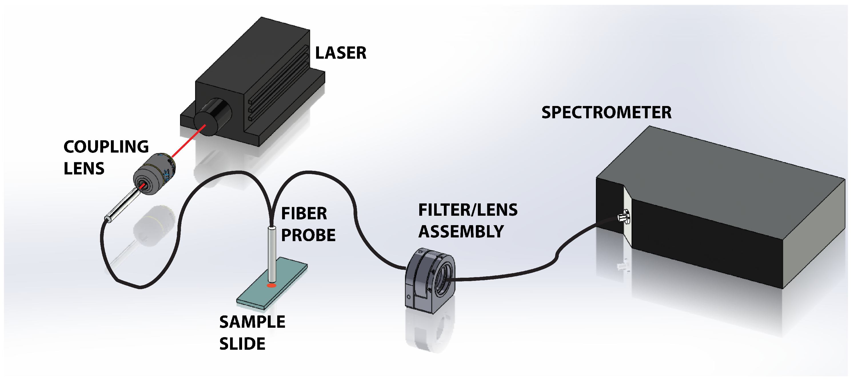
2.2. Apparatus
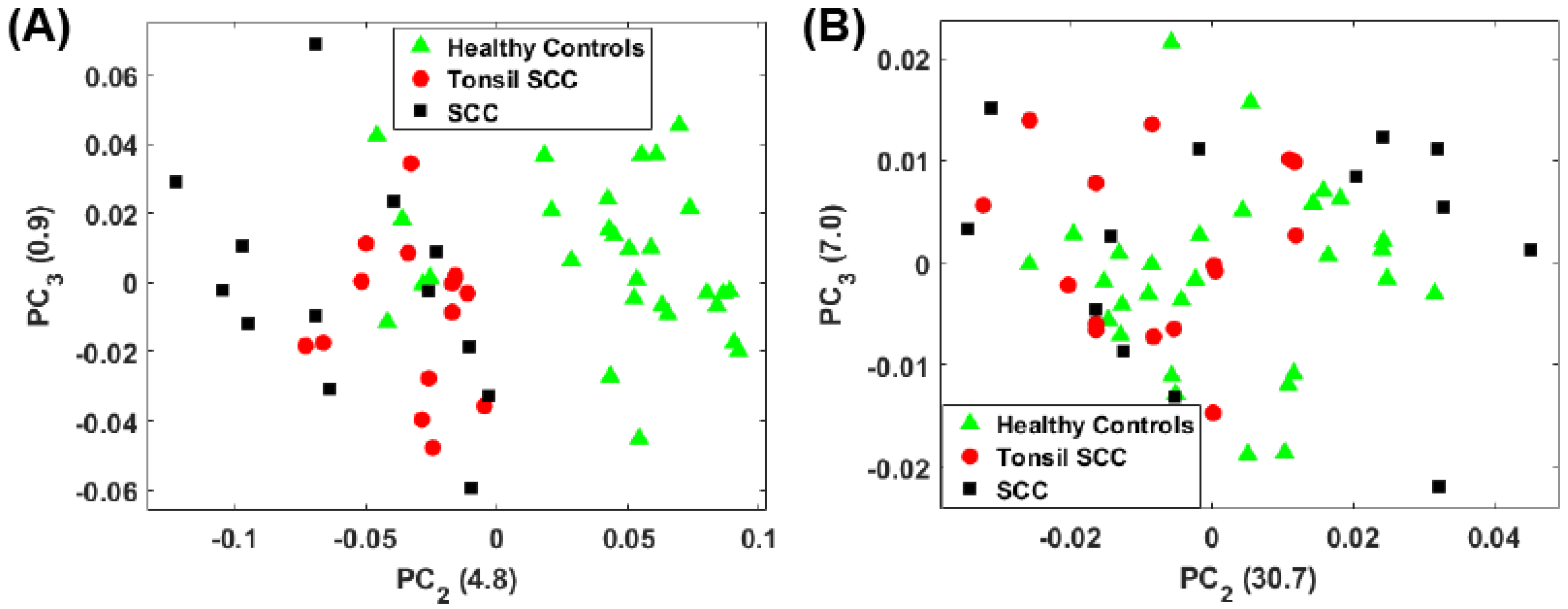
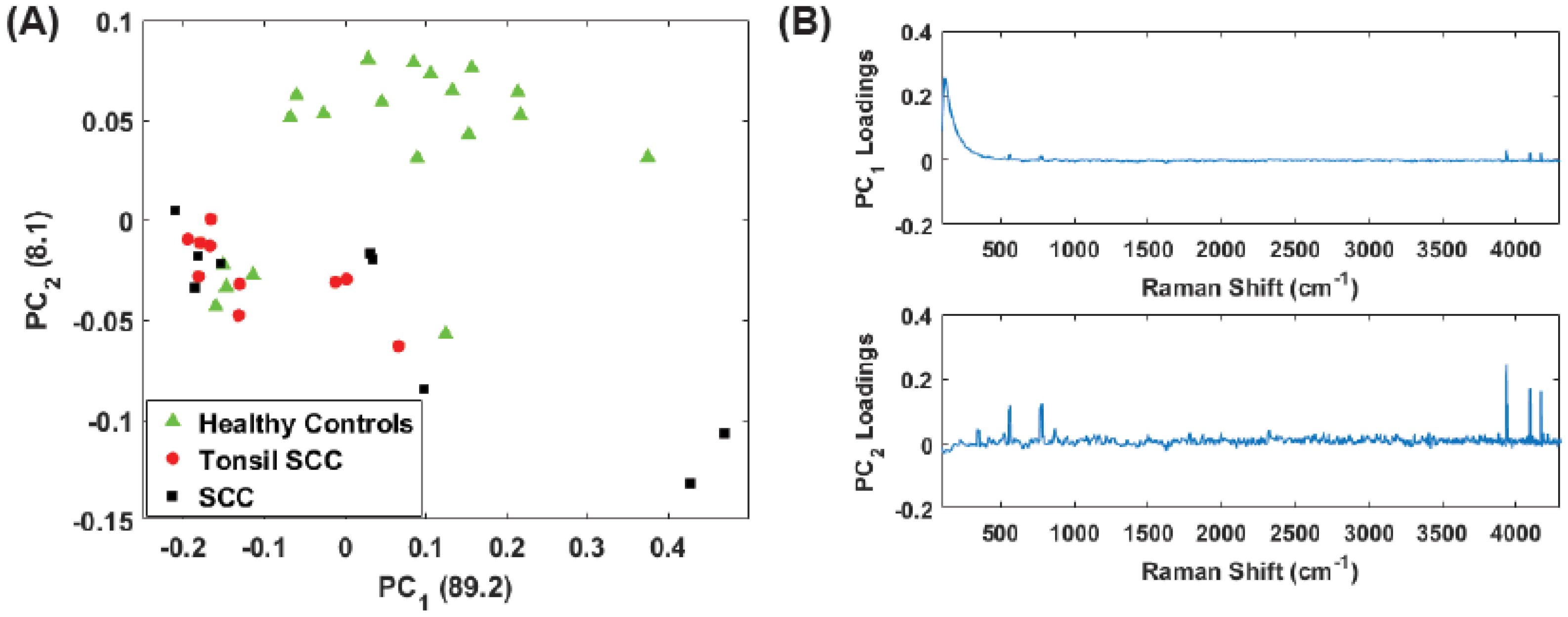
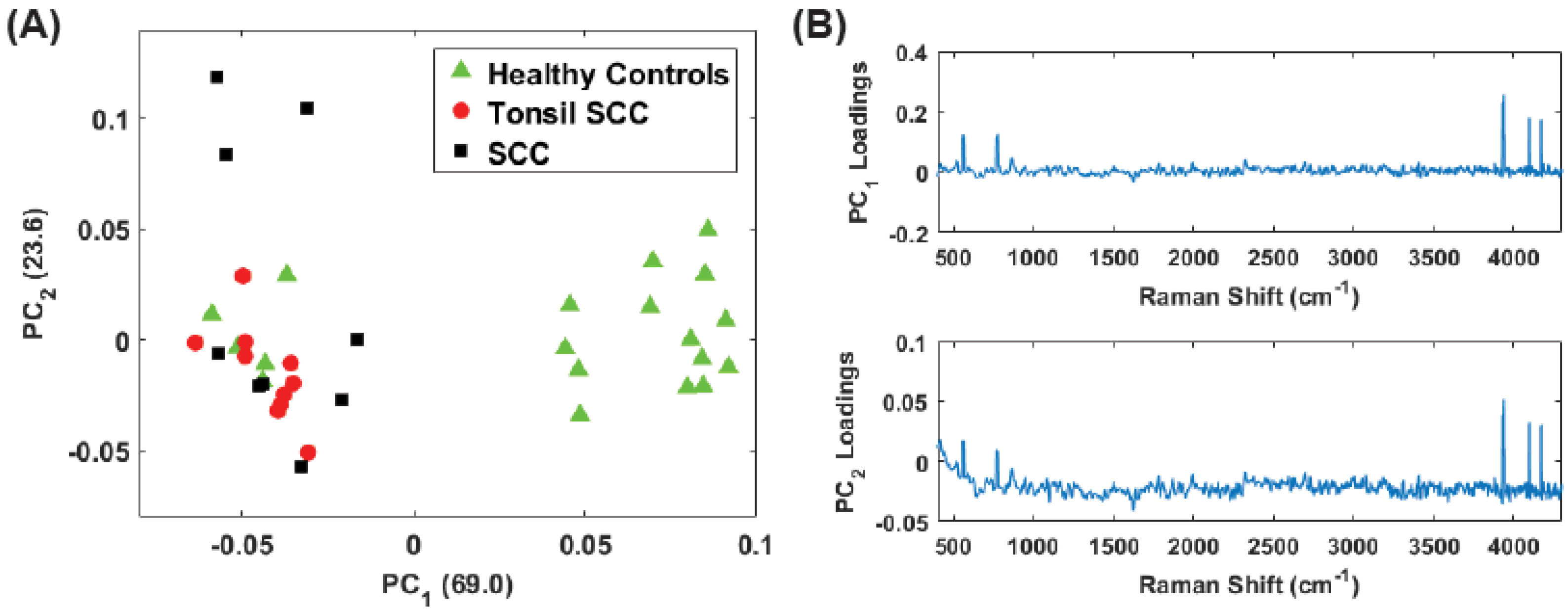
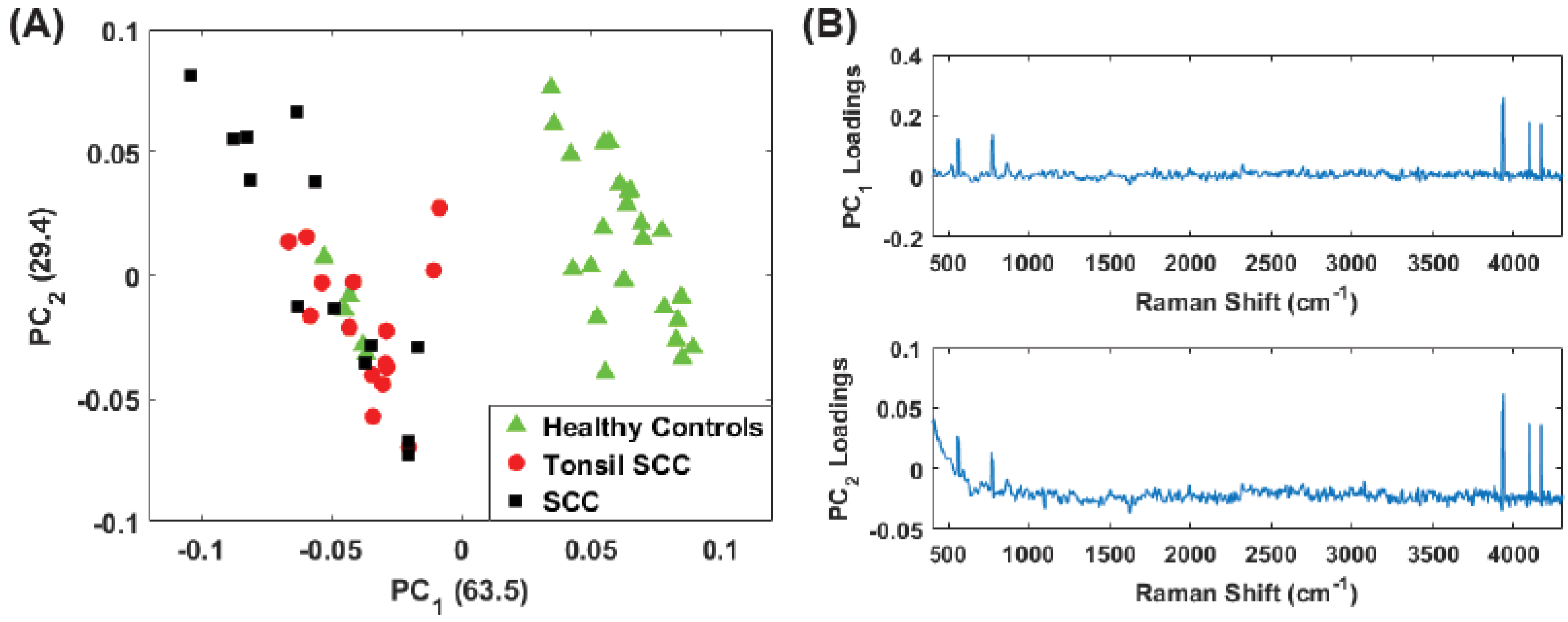
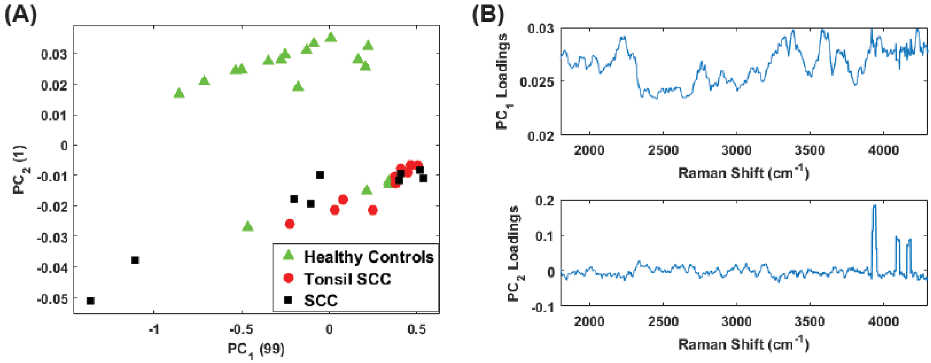
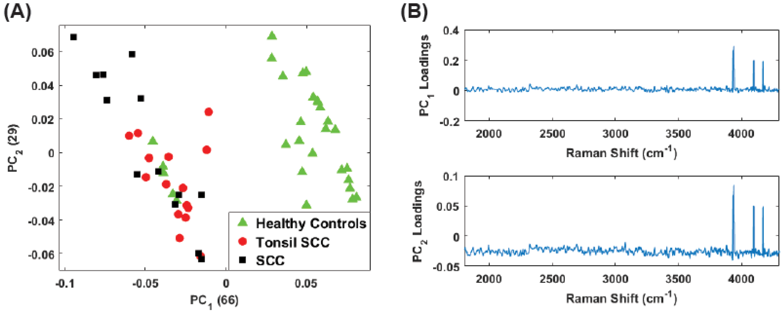
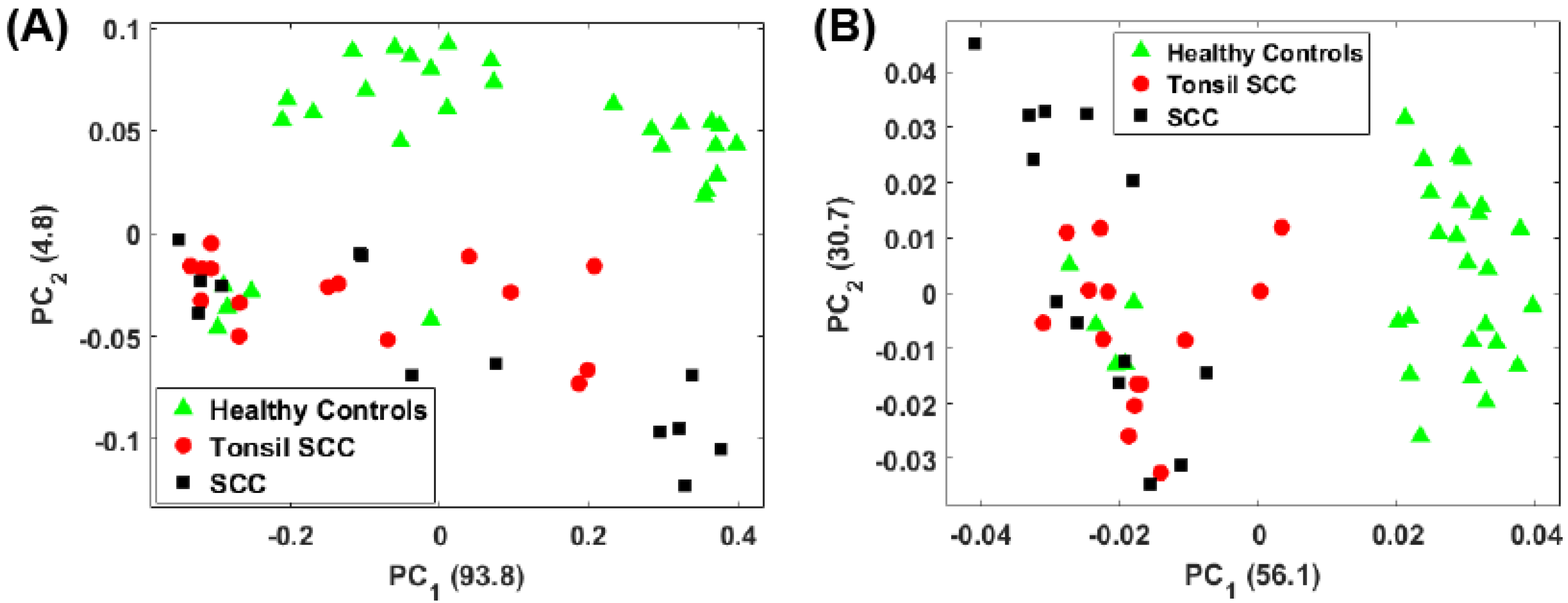
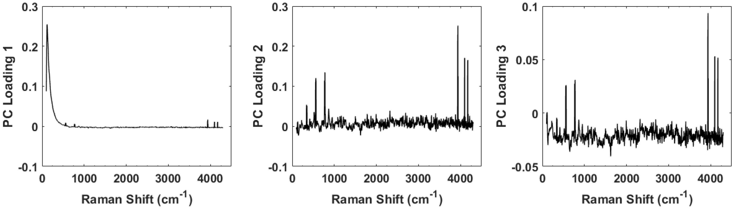
3. Principal Component Analysis
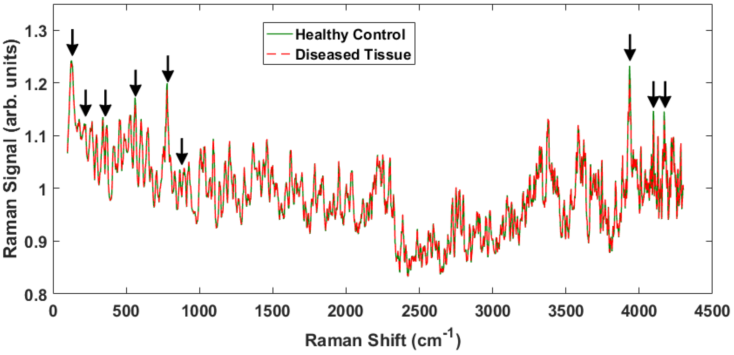
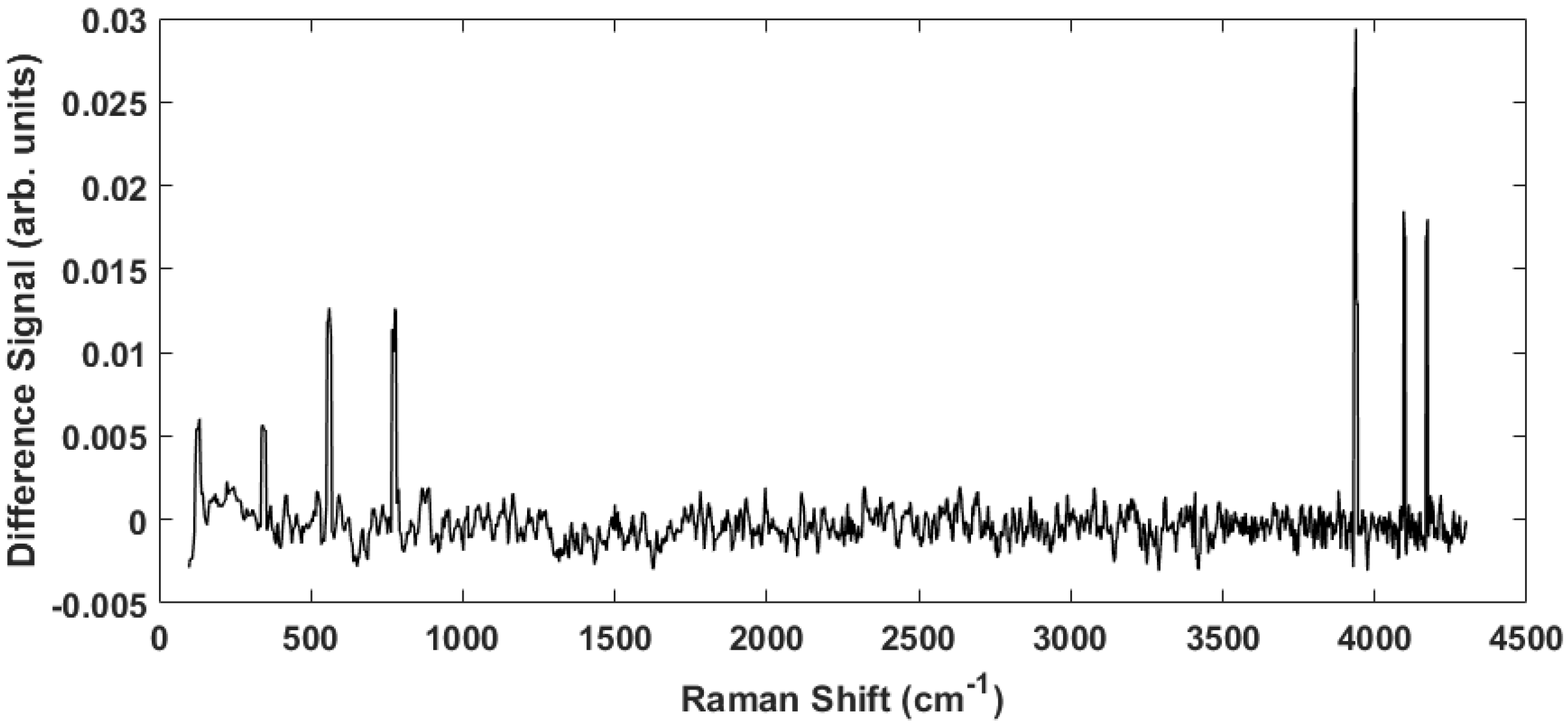
4. Results
5. Summary and Conclusions
Acknowledgments
Author Contributions
Conflicts of Interest
References and Note
- Jemal, A.; Bray, F.; Center, M.M.; Ferlay, J.; Ward, E.; Forman, D. Global cancer statistics. CA Cancer J. Clin. 2011, 61, 64–90. [Google Scholar] [CrossRef] [PubMed]
- Abogunrin, S.; DiTanna, G.L.; Keeping, S.; Carroll, S.; Iheanacho, I. Prevalence of human papillomavirus in head and neck cancers in European populations: A meta-analysis. BMC Cancer 2014, 14, 968. [Google Scholar] [CrossRef] [PubMed]
- Elrefaey, S.; Massaro, M.A.; Chiocca, S.; Chiesa, F.; Ansarin, M. HPV in oropharyngeal cancer: The basics to know in clinical practice. Acta Otorhinolaryngol. Ital. 2014, 34, 299–309. [Google Scholar] [PubMed]
- Calin, M.A.; Parasca, S.V.; Savastru, R.; Calin, M.R.; Dontu, S. Optical techniques for the noninvasive diagnosis of skin cancer. J. Cancer Res. Clin. Oncol. 2013, 139, 1083–1104. [Google Scholar] [CrossRef] [PubMed]
- Escobedo, J.O.; Rusin, O.; Lim, S.; Strongin, R.M. NIR Dyes for Bioimaging Applications. Curr. Opin. Chem. Bio. 2010, 14, 64–70. [Google Scholar] [CrossRef] [PubMed]
- Ardeshirpour, Y.; Chernomordik, V.; Capala, J.; Hassan, M.; Zielinsky, R.; Griffiths, G.; Achilefu, S.; Smith, P.; Gandjbakche, A. Using In-Vivo Fluorescence Imaging in Personalized Cancer Diagnostics and Therapy, an Image and Treat Paradigm. Technol. Cancer Res. Treat. 2011, 10, 549–560. [Google Scholar] [CrossRef] [PubMed]
- Harris, A.T.; Rennie, A.; Waqar-Uddin, H.; Wheatley, S.R.; Ghosh, S.K.; Martin-Hirsch, D.P.; Fisher, S.E.; High, A.S.; Kirkham, J.; Upile, T. Raman spectroscopy in head and neck cancer. Head Neck Oncol. 2010, 2, 26. [Google Scholar] [CrossRef] [PubMed]
- Krafft, C.; Dietzek, B.; Schmitt, M.; Popp, J. Raman and coherent anti-Stokes Raman scattering microspectroscopy for biomedical applications. J. Biomed. Opt. 2012, 17, 040801. [Google Scholar] [CrossRef] [PubMed]
- Knipfer, C.; Motz, J.; Adler, W.; Brunner, K.; Gebrekidan, M.T.; Hankel, R.; Agaimy, A.; Wil, S.; Braeuer, A.; Neukam, F.W.; et al. Raman difference spectroscopy: A non-invasive method for identification of oral squamous cell carcinoma. Biomed. Opt. Exp. 2014, 5, 3252–3265. [Google Scholar] [CrossRef] [PubMed]
- Wang, W.; Zhao, J.; Short, M.; Zeng, H. Real-time in vivo cancer diagnosis using Raman spectroscopy. J. Biophoton. 2015, 8, 527–545. [Google Scholar] [CrossRef] [PubMed]
- Tan, A.; Yildrimer, L.; Rajadas, J.; de la Pena, H.; Pastorin, G.; Seifalian, A. Quantum dots and carbon nanotubes in oncology: A review on emerging theranostic applications in nanomedicine. Nanomedicine 2011, 6, 1101–1114. [Google Scholar] [CrossRef] [PubMed]
- Mahadevan-Jansen, A.; Richards-Kortum, R. Raman spectroscopy for the detection of cancers and precancers. J. Biomed. Opt. 1996, 1, 31–70. [Google Scholar] [CrossRef] [PubMed]
- Su, L.; Sun, Y.F.; Chen, Y.; Chen, P.; Shen, A.G.; Wang, X.H.; Jia, J.; Zhao, Y.F.; Zhou, X.D.; Hu, J.M. Raman spectral properties of squamous cell carcinoma of oral tissues and cell. Laser Phys. 2011, 22, 311–316. [Google Scholar] [CrossRef]
- Devpura, S.; Thakur, J.S.; Sethi, S.; Naik, V.M.; Naik, R. Diagnosis of head and neck squamous cell carcinoma using Raman spectroscopy: Tongue tissues. J. Raman Spectrosc. 2012, 43, 490–496. [Google Scholar] [CrossRef]
- Singh, S.P.; Deshmukh, A.; Chaturvedi, P.; Murali Krishna, C. Raman spectroscopy in head and neck cancers: Toward oncological applications. J. Cancer Res. Ther. 2012, 8 (Suppl. 2), S126–S132. [Google Scholar] [PubMed]
- Guze, K.; Pawluk, H.C.; Short, M.; Zeng, H.; Lorch, J.; Norris, C.; Sonis, S. Pilot study: Raman spectroscopy in differentiating premalignant and malignant oral lesions from normal mucosa and benign lesions in humans. Head Neck 2014, 37, 511–517. [Google Scholar] [CrossRef] [PubMed]
- Valdés, R.; Stefanov, S.; Chiussi, S.; López-Alvarez, M.; González, P. Pilot research on the evaluation and detection of head and neck squamous cell carcinoma by Raman spectroscopy. J. Raman Spectrosc. 2014, 45, 550–557. [Google Scholar] [CrossRef]
- Cals, F.L.J.; Schut, T.C.B.; Hardillo, J.A.; de Jong, R.J.B.; Koljenović, S.; Puppels, G.J. Investigation of the potential of Raman spectroscopy for oral cancer detection in surgical margins. Lab. Invest. 2015, 95, 1186–1195. [Google Scholar] [CrossRef] [PubMed]
- Lin, K.; Zheng, W.; Lim, C.M.; Huang, Z. Real-time in vivo diagnosis of laryngeal carcinoma with rapid fiber-optic Raman spectroscopy. Biomed. Opt. Exp. 2016, 7, 3705–3715. [Google Scholar] [CrossRef] [PubMed]
- Lin, K.; Cheng, D.L.P.; Huang, Z. Optical diagnosis of laryngeal cancer using high wavenumber Raman spectroscopy. Biosens. Bioelectron. 2012, 35, 213–217. [Google Scholar] [CrossRef] [PubMed]
- Holler, S.; Wurtz, R.; Auyeung, K.; Auyeung, K.; Paspaley-Grbavac, M.; Mulroe, B.; Sobrero, M.; Miles, B.A. Ex-vivo holographic microscopy and spectroscopic analysis of head and neck cancer. In Proceedings of the SPIE 9328, Imaging, Manipulation, and Analysis of Biomolecules, Cells, and Tissues XIII, 93281L, San Francisco, CA, USA, 2 March 2015. [Google Scholar]
- The nonuniform thickness is a function of pathologic processing; these are real life samples from actual surgery, not controlled scientific samples. The thickness of the sections examined is at the discretion of the attending pathologist during the surgery and accounts for the variability.
- Andronie, L.; Mireşan, V.; Coroian, A.; Pop, I.; Raducu, C.; Rotaru, A.; Cocan, D.; Cîntă Pînzaru, S.; Domsa, I.; Coroian, C.O. Raman spectroscopy of the Hematoxylin-Eoisin stained tissue. ProEnvironment 2015, 8, 590–600. [Google Scholar]
- Johnson, R.A.; Wichern, D.W. Applied Multivariate Statistical Analysis; Prentice Hall: Upper Saddle River, NJ, USA, 1998. [Google Scholar]
- Rashid, N.; Nawaz, H.; Poon, K.W.C.; Bonnier, F.; Bakhiet, S.; Martin, C.; O’Leary, J.J.; Byrne, H.J.; Lyng, F.M. Raman microspectroscopy for the early detection of pre-malignant changes in cervical tissue. Exp. Molec. Path. 2014, 97, 554–564. [Google Scholar] [CrossRef] [PubMed]
- Ramos, I.R.M.; Malkin, A.; Lyng, F.M. Current Advances in the Application of Raman Spectroscopy for Molecular Diagnosis of Cervical Cancer. Biomed. Res. Int. 2015, 2015, 9. [Google Scholar] [CrossRef] [PubMed]
- Huang, Z.; McWilliams, A.; Lui, H.; Lam, S.; Zeng, H. Near-infrared Raman spectroscopy for optical diagnosis of lung cancer. Int. J. Cancer 2003, 107, 1047–1052. [Google Scholar] [CrossRef] [PubMed]
- Devpura, S. Raman Spectroscopy and Diffuse Reflectance Spectroscopy for Diagnosis of Human Cancer and Acanthosis Nigricans. Ph.D. Dissertation, Wayne State University, Detroit, MI, USA, 2012. [Google Scholar]
- Tuer, A.; Tokarz, D.; Prent, N.; Cisek, R.; Alami, J.; Dumont, D.J.; Bakueva, L.; Rowlands, J.; Barzda, V. Nonlinear multicontrast microscopy of hematoxylin-and-eosin-stained histological sections. J. Biomed. Opt. 2010, 15, 026018. [Google Scholar] [CrossRef] [PubMed]
- Bautista, P.A.; Yagi, Y. Digital simulation of staining in histopathology multispectral images: Enhancement and linear transformation of spectral transmittance. J. Biomed. Opt. 2012, 17, 056013. [Google Scholar] [CrossRef] [PubMed]
- Wang, H.; Boraey, M.A.; Williams, L.; Lechuga-Ballesteros, D.; Vehring, R. Low-frequency shift dispersive Raman spectroscopy for the analysis of respirable dosage forms. Int. J. Pharm. 2014, 469, 197–205. [Google Scholar] [CrossRef] [PubMed]
- Balandin, A.A.; Fonoberov, V.A. Vibrational Modes of Nano-Template Viruses. J. Biomed. Nanotech. 2005, 1, 90–95. [Google Scholar] [CrossRef]
- Talati, M.; Jha, P.K. Acoustic phonon quantization and low-frequency Raman spectra of spherical viruses. Phys. Rev. E 2006, 73, 011901. [Google Scholar] [CrossRef] [PubMed]
- Montagna, M. Brillouin and Raman scattering from the acoustic vibrations of spherical particles with a size comparable to the wavelength of the light. Phys. Rev. B 2008, 77, 045418. [Google Scholar] [CrossRef]
- Vehring, R.; Ivey, J.; Williams, L.; Joshi, V.; Dwivedi, S.K.; Lechuga-Ballesteros, D. High-sensitivity analysis of crystallinity in respirable powders using low frequency shift-Raman spectroscopy. In Proceedings of Respiratory Drug Delivery 2012; Dalby, R.N., Byron, P.R., Peart, J., Suman, J.D., Farr, S.J., Young, P.M., Eds.; Virginia Commonwealth University: Richmond, VA, USA, 2012; pp. 641–644. [Google Scholar]


| Patient | Tissue ID | Sex/Age | Diagnosis |
|---|---|---|---|
| 005094 | S01A | F/53 | Control |
| 005094 | S01B | F/53 | Tonsil SCC |
| 005112 | S01A | M/49 | Tonsil SCC |
| 005118 | S01A | M/49 | Tonsil SCC |
| 005120 | S01A | M/70 | Control |
| 005120 | S01B | M/70 | Control |
| 005120 | S01C | M/70 | SCC |
| 005120 | S01D | M/70 | SCC |
| 005120 | S01E | M/70 | SCC |
© 2017 by the authors. Licensee MDPI, Basel, Switzerland. This article is an open access article distributed under the terms and conditions of the Creative Commons Attribution (CC BY) license (http://creativecommons.org/licenses/by/4.0/).
Share and Cite
Holler, S.; Mansley, E.; Mazzeo, C.; Donovan, M.J.; Sobrero, M.; Miles, B.A. Raman Spectroscopy of Head and Neck Cancer: Separation of Malignant and Healthy Tissue Using Signatures Outside the “Fingerprint” Region. Biosensors 2017, 7, 20. https://doi.org/10.3390/bios7020020
Holler S, Mansley E, Mazzeo C, Donovan MJ, Sobrero M, Miles BA. Raman Spectroscopy of Head and Neck Cancer: Separation of Malignant and Healthy Tissue Using Signatures Outside the “Fingerprint” Region. Biosensors. 2017; 7(2):20. https://doi.org/10.3390/bios7020020
Chicago/Turabian StyleHoller, Stephen, Elaina Mansley, Christopher Mazzeo, Michael J. Donovan, Maximiliano Sobrero, and Brett A. Miles. 2017. "Raman Spectroscopy of Head and Neck Cancer: Separation of Malignant and Healthy Tissue Using Signatures Outside the “Fingerprint” Region" Biosensors 7, no. 2: 20. https://doi.org/10.3390/bios7020020