Article

Statistical Contact Angle Analyses with the High-Precision Drop Shape Analysis (HPDSA) Approach: Basic Principles and Applications

Department of Physical Chemistry, Saarland University, Saarbrücken 66123, Germany
*
Authors to whom correspondence should be addressed.
These authors contributed equally to this work.
Coatings 2016, 6(4), 57; https://doi.org/10.3390/coatings6040057
Submission received: 19 September 2016 / Revised: 20 October 2016 / Accepted: 28 October 2016 / Published: 6 November 2016
(This article belongs to the Special Issue Advances in Coatings Characterization)

Abstract

:
Surface science, which includes the preparation, development and analysis of surfaces and coatings, is essential in both fundamental and applied as well as in engineering and industrial research. Contact angle measurements using sessile drop techniques are commonly used to characterize coated surfaces or surface modifications. Well-defined surfaces structures at both nanoscopic and microscopic level can be achieved but the reliable characterization by means of contact angle measurements and their interpretation often remains an open question. Thus, we focused our research effort on one main problem of surface science community, which is the determination of correct and valid definitions and measurements of contact angles. In this regard, we developed the high-precision drop shape analysis (HPDSA), which involves a complex transformation of images from sessile drop experiments to Cartesian coordinates and opens up the possibility of a physically meaningful contact angle calculation. To fulfill the dire need for a reproducible contact angle determination/definition, we developed three easily adaptable statistical analyses procedures. In the following, the basic principles of HPDSA will be explained and applications of HPDSA will be illustrated. Thereby, the unique potential of this analysis approach will be illustrated by means of selected examples.

Graphical Abstract

1. Introduction and Brief Summary of Basic Wetting Theories

Investigating and analyzing the wetting behavior of solid surfaces has a long and controversially discussed history. Nowadays, drop shape analysis by contact angle determination of sessile drops is the preferred method to characterize solid surfaces in terms of wetting behavior [1,2,3,4], adhesion [5,6,7], surface topography and composition [8,9,10], superhydrophobicity [11,12,13], superolephobicity [14,15], wetting transitions [16,17], etc. Therefore, excellent summaries dealing with theoretical and practical aspects of contact angle determination and interpretation can be found in literature [18,19,20,21,22,23,24]. At the beginning of the 19th century, Thomas Young and Pierre Simon Laplace published their famous works “An essay on the Cohesion of Fluids [25]” and “Méchanique céleste [26]”, respectively, which resulted in two of the most famous equations in surface science, the Young equation and the Young–Laplace equation,
γ s , v Y o u n g = γ s , l + γ l , v × cos θ Y
Δ p L a p l a c e = Δ F A = γ α , β ( 1 R 1 + 1 R 2 )
The Young Equation (1) correlates the three interfacial tensions solid–vapor (s, v) solid–liquid (s, l) liquid–vapor (l, v) with the equilibrium contact angle θ Y in mechanical and thermodynamically equilibrium and the Young–Laplace Equation (2) depict the relationship between the difference in pressures between two phases α and β, which is given by the interfacial tension between the phases γ α , β and the curvature of the meniscus in terms of principal radii of curvature Ri. Both equations are strictly speaking only valid under mechanical and thermodynamically equilibrium conditions. Especially for droplets with small volumes and surfaces with low mechanic moduli such as polymer surfaces, additional parameters have to be considered, which were firstly introduced by Gibbs in his famous work “On the equilibrium of heterogeneous substances [27,28,29]” leading to the generalized Young and generalized Young–Laplace equation,
γ s , v g Y o u n g = γ s , v Y o u n g + ( κ s , l , v R 0 + d κ s , l , v d R 0 ) | cos φ s |
Δ p g L = Δ p L a p l a c e c 1 R 1 2 c 2 R 2 2 + Γ D × g × cos ϕ
λ i j = μ i j + z × g × M j
Equations (3)–(5) together form a dependent system of equations, which describe the mechanical and thermodynamically equilibrium of a three phase system at the three phase interphase (≡ triple line) (Equation (3)) with values of line tension κ s , l , v (≡ three phase interfacial tension) and the angle between the substrate surface and the local principal plane of the three phase contact line φ s , the shape of the two phase interphase (Equation (4)) with curvature constants ci, absolute adsorption Γ D , gravity acceleration g and the angle relative to the gravitational field ϕ and the influence on the chemical potential μ i j depending on the elevation in the gravitational field z (Equation (5)). Especially the influence of the gravitational potential on the shape of the two phase interphase and on the magnitude of the equilibrium contact angle is critically discussed in surface science community [30,31,32,33,34,35,36]. However, in every case, a contact angle is needed to get inside the thermodynamic theories. Due to the fact that wetting experiments by sessile drop techniques generally cannot be performed under mechanical and thermodynamically equilibrium conditions, the equilibrium contact angle cannot be measured directly. Indeed, the measured or apparent contact angles (APCA) differ considerably from each other, which is denoted as Contact Angle Hysteresis (CAH) [37,38,39,40,41] in surface science community. The contact angle hysteresis can be calculated by the experimental available advancing θa (wetting new surface) and receding θr (formerly wetted surface), which together determine the CAH,
Δ θ = θ a θ r 0
For real solid surfaces, the CAH given by Equation (6) is always larger than zero. Furthermore, the Young and generalized Young equation are only valid for “ideal” surfaces, which means isotropic, atomically flat, chemically non-reactive, rigid and non-deformable. However, real solid surfaces are generally rough and heterogeneous. First attempts to consider the real surface structure in terms of physical roughness and heterogeneity were introduced by Wenzel [42] and Cassie and Baxter [43] resulting in the Wenzel (Equation (7)) and Cassie–Baxter equations (Equation (8)),
cos θ W = r W × cos θ Y ;   r W = A r e a l A g e o m 1 ;   A g e o m = b × l
cos θ C B = r f × f × cos θ Y + f 1
Both equations are not easy to handle and a lot of experimental effort has to be spend to determine the roughness ratio of the surface rw or rf and the fraction of the solid surface wetted by the liquid f. The Wenzel equation refers to a homogeneous wetting state that means the liquid on the surface enters grooves and totally covers the wetted surface. This state is also denoted as “Wenzel wetting state” [44,45] and connects the measured contact angle θW with the equilibrium contact angle by defining a roughness factor rW. The Cassie–Baxter equation refers to a heterogeneous wetting state that means the liquid not totally wets the surface because air trapped grooves between the surface and liquid are present. This state is also denoted as “Cassie wetting state” [44,45]. Obviously, no distinction between wetting and dewetting of the surface is taken into account in both Equations (7) and (8), because the well-known experimentally observed advancing and receding contact angles were not considered. Therefore, the question to be answered is the connection between the experimental available advancing and receding contact angles and the equilibrium contact angle. Many efforts were spend to answer this question. For example, Tadmor [46] proposed Equation (9), which connects the equilibrium contact angel with the advancing and receding contact angles on a real smooth (finitely rigid surface) surface,
θ Y = arccos ( r A × cos ( θ A ) + r R × cos ( θ R ) r A + r R ) ;   r A , R = ( sin 3 θ A , R 2 3 × cos θ A , R + cos 3 θ A , R ) 1 / 3  
where θ A represents the advancing and θ R represents the receding contact angle. Kamusewitz and Possart [47] proposed an empirical model to determine the equilibrium contact by measuring advancing and receding contact angles on different rough low-energy surfaces. They proposed a linear relationship between surface roughness and contact angle hysteresis resulting in Equations (10) and (11),
θ a = θ Y + A a × Δ θ
θ r = θ Y + A r × Δ θ
By plotting the experimental data of θa, θr against ∆θ and linear extrapolation using Equations (10) and (11) to ∆θ = 0 (≡ corresponds to the y axis intercept), this “hysteresis-free” contact angle value is considered as thermodynamic equilibrium contact angle. In a more theoretical approach, Kamusewitz and Possart [48] derived a relationship between CAH and Wenzel’s contact angle by introducing the Wenzel equation into the Young equation, leading to Equation (12),
cos θ W = 0.5 × ( cos θ a + cos θ r )
By determine the roughness factor by, e.g., scanning force microscopy, the equilibrium contact angle can then be calculated by using the Wenzel Equations (1)–(7). At this point one critical fact has to be stressed that is the chemical heterogeneity of a real surface, which is also highlighted in the cited contributions. A real surface cannot generally be considered as homogeneous on the micro- or nanoscale. Surface defects, coating defects, different crystal structures, impurities, adsorption, different compounds, etc. generally lead to a surface with varying solid–vapor interfacial tension γs,v. According to Equations (1) and (3), a varying solid–vapor interfacial tension affects the force balance at the three phase interface and therefore the magnitude of the equilibrium contact angle. That means that generally more than one equilibrium contact angle exists on every real surfaces and the experimenter of contact angle measurements should therefore be very carefully before claiming that the measured or calculated contact angle by the above described approaches represents the equilibrium contact angle of the surface. The question of determination of a reproducible, representative CA (often referred as equilibrium, thermodynamic CA) is since today one of the most critically discussed and most interesting topics in surface science. Since today, the presence of local inhomogeneities and their influence on the contact angles or the motion behavior of the triple line are considerably less well understood. Some scientists spend a lot of effort and theoretically discussed the topic. For example, Joanny and de Gennes [49] proposed a theoretical model that related the contact angle hysteresis to local energy defects (patches with different surface energies) on a smooth surface. Shanahan [50] theoretically discussed the behavior of the triple line on a heterogeneous surface with randomly distributed circular flaws of high surface energy. Marmur [51] illustrated in great detail that the wide range of apparent contact angles on heterogeneous surfaces is caused by multiple local and global energy minima of the Gibbs energy curve for a liquid drop on such a surface and discussed theoretically the possibility to use the contact angle hysteresis to detect chemical nano-heterogeneities of the order of magnitude of 10 nm [52]. Generally, the influence of surface roughness and surface heterogeneity/varying interfacial tension on the measured contact angles cannot be separated. Another influencing factor, which is obviously often ignored, especially by people using contact angles as measuring tool, is “the way the contact angles were measured”. The procedure to determine, e.g., advancing and receding angles strongly depends on the used equipment and on several subjective criteria of the operator like frame rate of the video recording, resolution of the CCD-camera, drop volume, temperature, humidity, used specific contact angle definition (after or before the movement of the triple line), etc., which unfortunately are often not named in detail. Beside these critical parameters, the results and interpretation of contact angle measurements depend even on the measuring technique its selves (e.g., horizontal setup vs. inclined setup [53,54,55]). Especially the retention force, which is required to slide a drop on a surface and therefore contact angle variation, also depends on the resting time before the droplet starts to slide [56] and on the drop size [57]. Other critical points are the used image analysis fitting procedures to determine apparent contact angles. Beside the Young–Laplace or Bashford–Adams fitting, common software fit one circle/ellipse or polynomial functions (tangential) onto the macroscopic drop shape. These approaches work quite well for static and axisymmetric droplets, e.g., by axisymmetric drop shape analysis ADSA [58,59,60] in its various versions but fail if strongly non-axisymmetric droplets during contact angle measurements are evaluated. In addition, pixel resolutions and the generally performed discretization of the images affect the ADSA procedure [61]. Other more advanced approaches use direct image processing methods or are based on local edge interpolation or fitting [62]. As a result, it is not an easy task to determine the magnitude of the contact angle hysteresis for a solid surface in a reproducible manner. Thus, there exist many misleading concepts presented in the scientific literature concerning some aspects of contact angle topic, even in the highly cited papers. This fact was recently highlighted by Volpe et al. [63]. In this regard, we developed a special calculation and evaluation strategy for contact angle measurements and wetting experiments, which is named high-precision drop shape analysis (HPDSA) [64]. An intention of the complete procedure (the combination of HDPSA and CA analyses) was allowing the user to determine valid and reproducible contact angles, which are free of any subjectivity of the operator. A broad diversity of biological, physical, and chemical effects involve wetting events so that this question is most important for the small community itself but especially for all the multiple “users” of sessile drop experiments/of the optical observation of contact angles. The HPDSA was developed to be especially suitable for highly asymmetric drop shapes because no “physically sound” and really satisfactory technique for contact angle measurements in case of non-axisymmetric drops was at present available. Beside the high-precision contact angle calculation independent on drop symmetry, the complex transformation of drop shape images in Cartesian coordinates (non- or less discretization than edge determinations) makes using every known mathematical approach to calculate contact angles (even ADSA) possible. To analyze the set of measured contact angle data, we developed different statistical analyses strategies for contact angle measurements, which lead to characteristic wetting parameters and detailed information about the surface, instead of “just measuring an angle”. This information can be used, e.g., to enhance coating processes and qualities, to design surface applications, etc. Basic principles of the HPDSA procedure will be summarized in the following sections. The reader should note that the presented strategies for the contact angle analyses are not restricted to the HPDSA approach and of course can also be performed with commercial contact angle analysis software. Furthermore, the HPDSA technique can also be applied to asymmetric drops that are in a centrifugal adhesion balance [65,66,67,68,69], which is a very interesting and useful technique to measure, e.g., the lateral adhesion force at the solid–liquid interface. In the experimental section, selected examples for different applications of HPDSA will be presented. Thereby, drop shape extraction, static, dynamic and statistical contact angle analyzes will be presented by examples of real smooth surfaces, contact angle hysteresis, dynamics of wetting, wetting on rough and chemically heterogeneous surfaces, superhydrophobic and rose petal-surfaces, nonstick droplets and sticking droplets (ionic liquids).

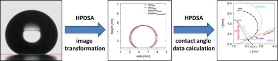
2. Basic Principles of HPDSA

The basic information about the HPDSA procedure can be found in publication [64]. To avoid confusion, a summary of all used symbols, variables and parameters within this contribution can be found in the Abbreviations Section. The used OCA20 contact angle measuring system leads to one avi video file per measurement, which is converted in loss-free bmp images using the freeware program VirtualDub v1.9.11 1998–2010 (vitualdub.org) by Avery Lee or a LabVIEW routine but every commercial software can be used to create an image sequence. The bmp image sequence is the starting point of the HPDSA software (M. Schmitt, Völklingen, Germany), in which the HPDSA procedure is implemented.

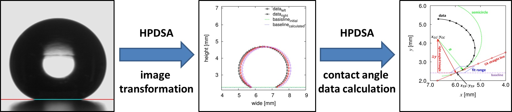
2.1. Image Transformation and Drop Shape Extraction

The bmp format/color code contains three hexadecimal numbers between “00” (≡ black) and “FF” (≡ white), which represent the color of a pixel. In a first step, the hexadecimal code is translated in x- and y- direction in the RGB color code, which ranges from please check “0 0 0” (≡ black) to “255 255 255” (≡ white). Afterwards, the sum of color values col is determined, which ranges from “0” (≡ black) to “765” (≡ white). Due to the fact that the used bmp image sequence contains only greyscale images, every greyscale has its defined sum of color value and different greyscales can never have the same sum of color value. This fact is the basis for the color/drop shape detection with HPDSA. The next step is a dynamic linear regression in x- and y- direction of three and of five neighboring points n = 3, P ε {0, 1, 2} and n = 5, P ε {0, 1, 2, 3, 4} to determine the rates of color p for every pixel using Equation (13),
d   c o l d   P = ( c o l i × P i ) × n c o l i × P i n × P i 2 ( P i ) 2 = p x , y
At this point, one grey-scale image is dynamically transferred in 440832 six-dimensional points. To detect the drop shape, only points with rate values that significantly differ from 0 in both regressions are considered. The detection limit (≡ resolution) of the procedure is manually definable by the user by setting a limit value lv (≡ minimal rate of color value). An example for different color transitions and corresponding color rate values is given in Table 1.
As illustrated by Table 1, the three-point regression is more specific to the position (Numbers 2–3, Numbers 12–13 ≡ white to black transitions) but is also more affected by noise (Numbers 7–9). The five-point regression is less specific to the position but is less affected by noise so that it is used for noise correction during the procedure. However, even in an ideal case (≡ white to black transition, Numbers 2–3 and Numbers 12–13), the procedure will result in at least two points for one step in color (Table 1, Numbers 4–5). Therefore, a weighting procedure depending on the color rates px and py in both directions is performed by applying Equation (14),
E ( x ) = ( x i × p x i ) p x i   ;   E ( y ) = ( y i × p y i ) p y i
resulting in color rate weighted expectation values E(x) and E(y). Furthermore, standard deviations are calculated using Equation (15),
σ ( x ) = p x i p x i × ( x i E ( x ) ) 2   ;   σ ( y ) = p y i p y i × ( y i E ( y ) ) 2
resulting in a converted drop shape, which is transferred by multiplying with the scale factor of the image in Cartesian coordinates with sub-pixel resolution (μm coordinates).

2.2. Baseline Detection and Triple “Point” Determination

The baseline (correctly speaking the projection of the triple line, see below) of a sessile drop is an important parameter for the contact angle calculation, triple point determination, etc. Hence, the accuracy of the baseline determination is a crucial step during the procedure. During the HPDSA process, the baseline is detected by fitting two linear functions per side of the droplet, one for the real drop shape and one for the mirrored drop shape/reflection from the surface, with a distance between 1 and 10 pixels (<200 μm) from a given initial baseline. The intersection points of both functions determine the baseline so that the baseline can be calculated for every drop image of the measurement. This dynamic control of the baseline is especially suitable, if, e.g., the drop shape is slightly shifted/tilted during the measurement (non-horizontal baseline). Alternatively, average values for the baseline from approximately 40% of the drop images can be calculated, which results in an average baseline. This is especially suitable if the measurement is strongly affected by image fluctuations like noisy signal processing. The determined points for the baseline can generally be used for the triple point detection (note that the notion “triple point” refers to the position of the 3D triple line in the 2D projection of the drop image). However, these coordinates can be slightly shifted in x-direction from the real triple points depending on the contact angle (curvature of the meniscus) and the resolution of the mirrored drop shape. Therefore, the coordinates of the triple points XTP and YTP are computed as intersection point of the extracted drop shape with the baseline, Equations (16)–(19),
T 1 = R 2 ( b Y M P ) 2 X M P 2 1 + m 2
T 2 = b × m Y M P × m X M P 1 + m 2
X T P = ± ( T 1 T 2 ) 2 T 2
Y T P = m × X T P + b
where m and b are the slope and the axis intercept of the baseline, respectively, and XMP,YMP define the mean radius R and the center of a fitting semi-circle (compare to Section 2.4). The physically practical signs in Equation (18) depend on the considered side of the droplet (+ ≡ right side of the droplet; − ≡ left side of the droplet).

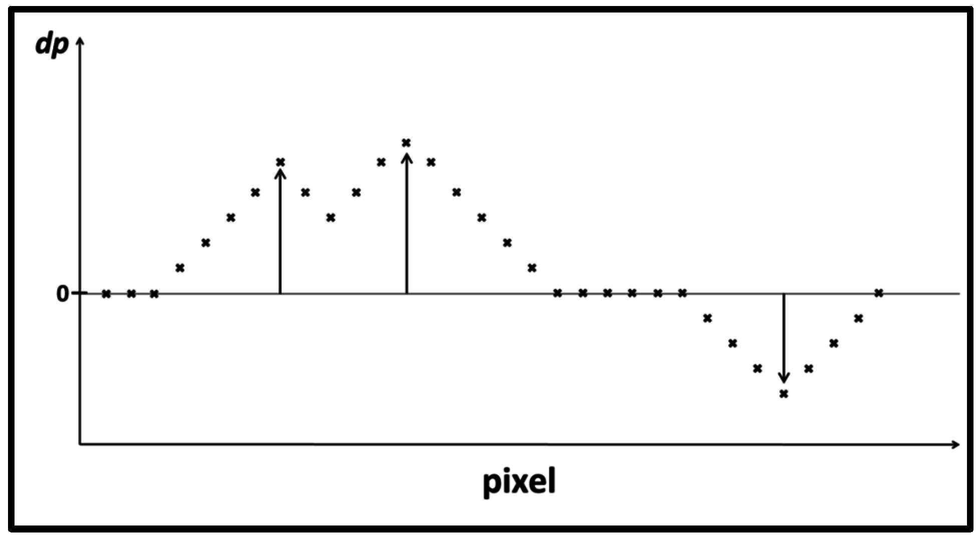
2.3. Noise Elimination

To be able to extract drop contours and to calculate contact angles with high-precision, the noise elimination, e.g., due to illumination effects, reflections, etc., is an important point. The inner reflection due to the illumination of the droplet is removed by a dynamic elliptical area using Equation (20),
Y 1 / 2 = Y E C ± R y 1 ( x X E C R x ) 2
with XEC;YEC being the center points of the ellipse and Rx;Ry being the radii of the ellipse, which can be defined by the user. More critical are noise and reflection effects, which occur distant from the center of the ellipse, e.g., at the drop contour. To remove noise near the drop contour, the HPDSA program contains an algorithm, which is based on the weighting procedure described in Section 2.1. Firstly, the maxima and minima of the color rate values pxi ≡ dp are identified Then, for every affected coordinate x, the ratio of distances from the minimum and the value of both maxima are taken into account. The influence of the second point W2 on the first point W1 = 1 − W2 before the minimum can be approximated applying Equations (21) and (23),
a ( x ) = P 2 m a x P 1 m i n P 2 m i n x
b = d p 2 m a x d p 1 m a x + d p 2 m a x
W 2 ( x ) = a ( x ) × b a ( x ) × b + ( 1 a ( x ) ) × ( 1 b )
By modifying the rate values pxi with the corresponding influencing factor Wi(x) and performing the weighting procedure explained in Section 2.1, this approach is able to separate adjacent points, as schematically illustrated in Figure 1.
Of course, hardware-restricted influences on the image quality cannot be fully compensated. Therefore, optical hardware with highest precision is mandatory for high-precision analyses but the procedure also can lead to better results for faster devices with lower precision. Currently, a complex image correction using an internal standard and a more sophisticated regression procedure (2D area regression) taking both directions simultaneously into consideration are tested, which might further enhance the noise elimination.

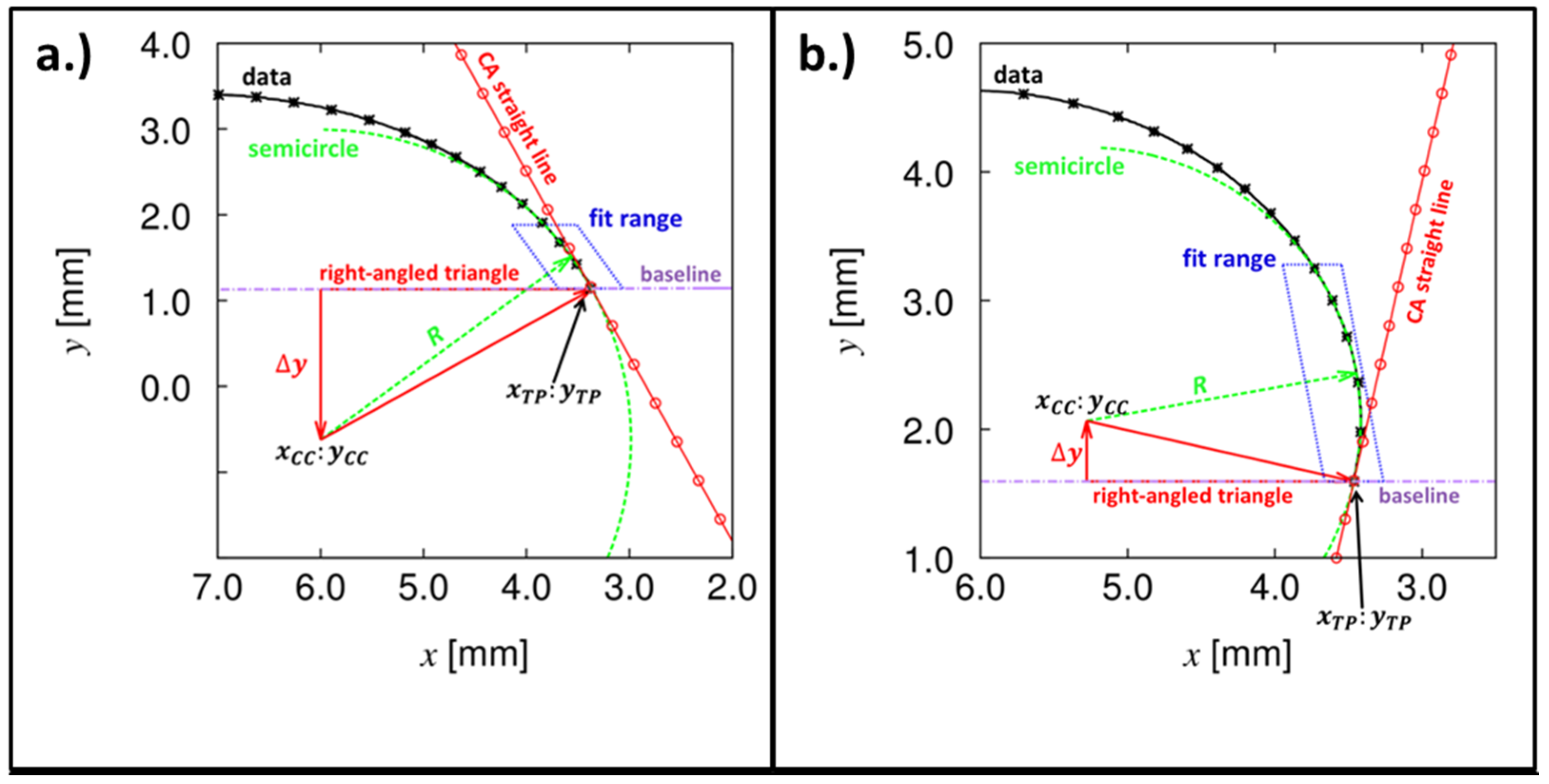
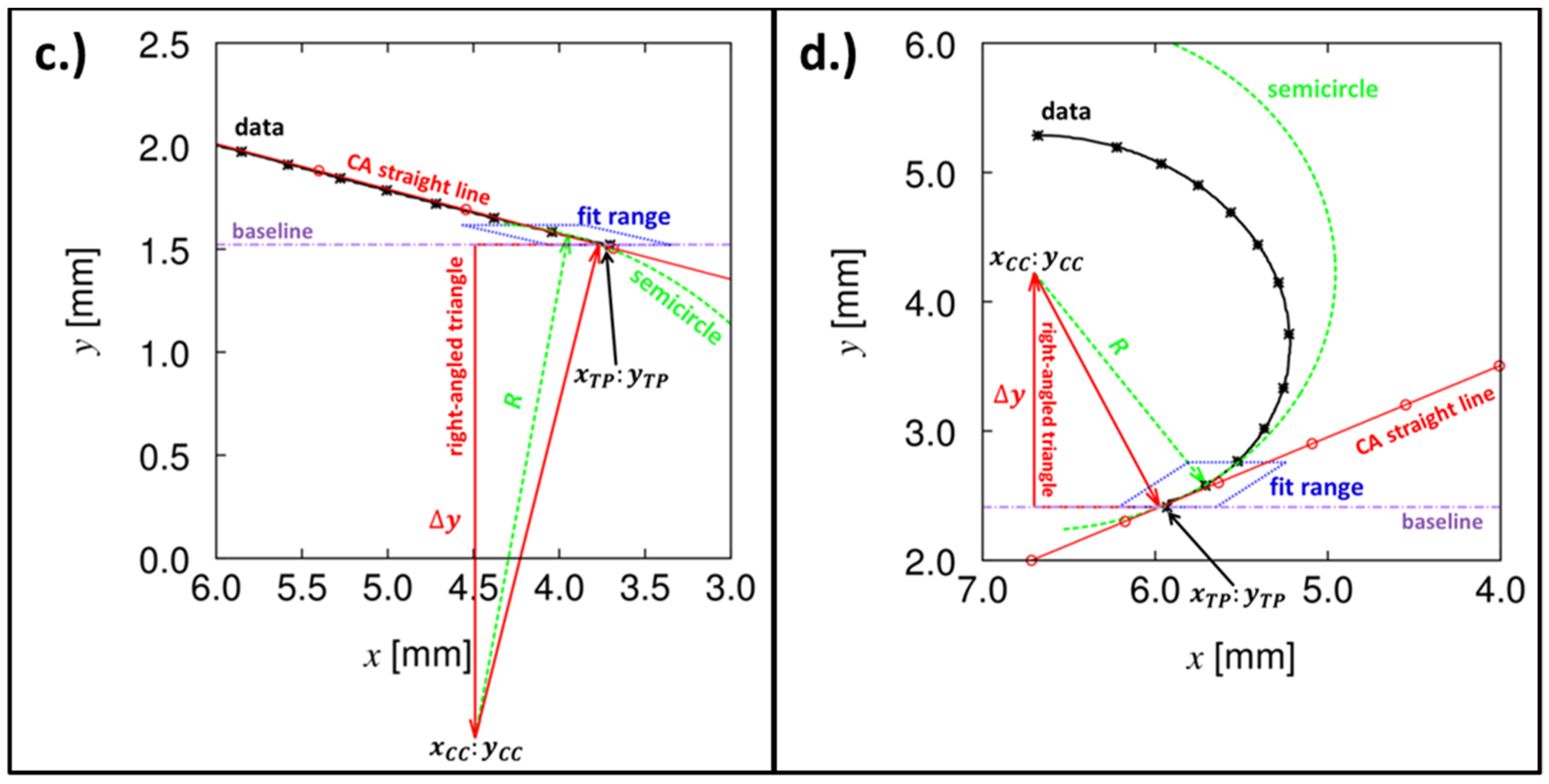
2.4. Fitting Procedure and Contact Angle Calculation

The theoretical drop shape is given by Laplace and generalized Laplace, Equations (1) and (4), respectively, which contain a circular function. According to Equations (2) and (4), the curvature of every single point of the drop is of interest. In this regard, a semi-circle function is used in HPDSA to adapt the radius R for one radius of curvature of the 2D projection using Equation (12),
y 1 / 2 = y c c ± R 2 ( x x c c ) 2
where xcc, ycc determine the center of a fitting-circle. To be able to calculate contact angles larger than 90°, exchanging of the x- and y-axes of the Cartesian coordinate system takes place (rotation by 90°). Otherwise, contact angles of 90° would result in rates tending towards ± infinity. During this procedure, the drop shape is split in two parts (right and left) at the highest point of the drop shape (xmax:ymax). The advantage is that both sides of the drop shape can be fitted individually, allowing the analysis of even highly non-asymmetric drop shapes of sticking droplets, e.g., during inclining-plate measurements. The least-squares fitting procedure takes place using a non-linear least-squares algorithm, which is, e.g., implemented in gnuplot software v.4.6 (www.gnuplot.info) 1986–2012. Because all parameters in Equation (24) are correlated, the convergence of the fitting procedure is a critical point and has to be carefully controlled. Therefore, the HPDSA use the variation of the minimal length of the calculation arc d arc , which is given by Equation (25),
d a r c = ( Y B 1 Y B 2 ) 2 + ( X B 1 X B 2 ) 2
which is definable by the user (≡ fitting range). The program calculates the boundary points XB1:YB1 and XB2:YB2 of the fitting procedure starting with the triple points XTP:YTP which leads to the real length of the calculation arc of every circle barc, Equation (26),
b a r c = 2 × π × R × β a r c 360 °
The angle β a r c is the angle between the vectors d B 1 : C C and d B 2 : C C (≡ vector from boundary points to the center of the circle) and can be calculated using the cosine theorem, Equation (27),
d a r c 2 = d B 1 : C C 2 + d B 2 : C C 2 2 d B 1 : C C 2 × d B 2 : C C 2 × cos β arc
with the lengths of the vectors equal to R. An additional benefit of the adaption of the primary radius of curvature R is the possibility for a tangent-free calculation of contact angles. Therefore, the sine theorem can be used in a right-angled triangle, Equation (28),
θ m = 90 ° + arcsin ( Δ y R ) ± α B L
where α B L is the inclination angle of the baseline (to correct non-horizontal baselines) and Δ y is the difference in height coordinates between the triple points and the center of the fitting circle. A schematical visualization of the fitting procedure and the contact angle calculation is illustrated in Figure 2.
To be able to calculate the whole range of practical contact angles ( 0 ° < θ m < 180 ° ), the newest version of HPDSA contains a “Fast-Circle-Fit” subroutine. Due to the nature of the circle function, Equation (29),
R 2 = ( x x c c ) 2 + ( y y c c ) 2
where three representative points are sufficient to calculate good starting values for the radius of the fitting circle to keep the time exposure of the main routine as low as possible. The computed points are the result of least squares multipoint polynomial (2nd order) regression of data points at the start, middle and end of the fitting range. The FCF-routine do not have the same accuracy as the main fitting routine in the “normal” contact angle range between ≈ 20° < θ m < 120° but is especially suitable for small contact angles ( θ m 20 ° ) and to analyze changes in curvature direction (convex to concave).

3. Materials and Methods

Detailed information about the experimental procedures and analyses can be found in the corresponding publications concerning contact angle measurements [64,71,72,73,74,75,76,77,78], the surface preparation by straight-forward gas phase silanization [71,73,74,75,76,78], AFM analyses [71,73,74,75,76,78], FTIR analyses [78] and spectroscopic ellipsometry analyses [75]. In the following, only the general procedure of contact angle measurements will be described.

Contact Angle Measurement

The general measurements of contact angles was performed as follows: Contact angle determination took place on horizontal surfaces by changing the drop volume (by adding and/or reducing) or continuously inclining the sample surfaces with and angular speed of φ = 0.59°/s (inclining-plate technique), using an OCA20 measuring system (Dataphysics, Filderstadt, Germany). The system is mounted on vibration-free desk to reduce the noise from natural building vibrations. Thereby, a sufficient volume of ultra-pure test-liquids (between 0.03 mL and 0.05 mL) under saturated vapor atmosphere of the test liquid (closed measuring chamber with definable measuring positions) was video recorded with a frame rate of 25 frames per second. To enlarge the population for statistical analysis and to ensure reproducibility, the measurements were repeated on ten defined measuring positions for each surface and with each liquid. To distinguish between horizontal and inclined measuring setup’s, the advancing angles θ a on an inclined plate are denoted as downhill angles θ d (measured at the right edge of the droplets) and the receding angles θ r are denoted as uphill angles θ u (measured at the left edge of the droplets).

4. Applications of HPDSA

In the following section, the application of HPDSA to different topics concerning contact angle analyses and data generation will be illustrated by using selected examples of our research activity during the last years. The scope of this section is to motivate the reader to perform contact angle measurements in a controlled and reproducible manner and to illustrate the potential of contact angle measurements in combination with a meaningful analysis strategy to extract additional information on the surface/coating, which can be used, e.g., to enhance coating processes and qualities, to design and enhance surface applications instead of just measuring “some contact angles”.

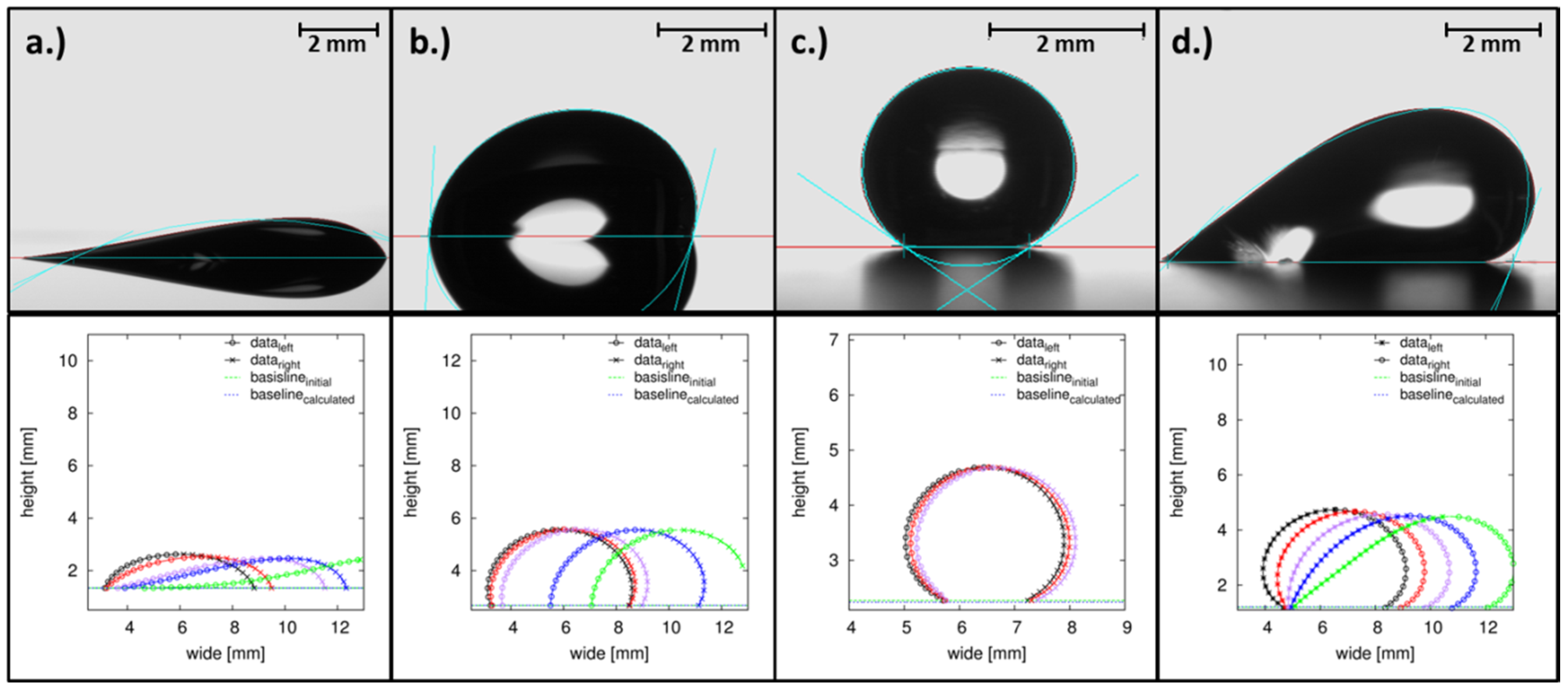
4.1. Drop Shape Extraction and Contact Angle Calculation

The reproducible extraction of the experimental drop shape is the basic but crucial factor for a meaningful contact angle calculation. Whereas generally axisymmetric drop shapes are uncomplicated, the reproducible characterization of non-axisymmetric drop shapes is much more complicated. The famous ADSA technique [58,59,60] and its various versions is the method of choice for axisymmetric drop shapes (e.g., pendant drop) but is due to its nature not applicable to non-axisymmetric drop shapes. Unfortunately, every real surface tents to lead to non-axisymmetric drops even without inclining the sample. Most coating applications involve extreme wetting situations such as extreme low contact angles near spreading (θm < 20°), non-sticking droplets on superhydrophobic surfaces with θm > 150° or sticking droplets on rose petal surfaces with extreme large contact angle hysteresis and therefore high asymmetry. Most of commercial contact angle analyzing procedures/software’s are not able to evaluate these quantities in a reproducible manner because the whole drop shape is considered for the analyses. Due to high-resolution coordinate’s transformation, drop splitting and definition of the fitting range near the triple line, HPDSA is able to extract drop shapes and to calculate contact angles over the entire practical contact angle range between 0° < θm < 180°. A few examples for different wetting situations are illustrated and compared to the commercial SCA20 analysis software in Figure 3. The images were recorded with the same magnification, whereas approximately 59 Pixels corresponds to a distance of 1 mm.
As illustrated in Figure 3, the SCA20 software results in a large error by calculating the contact angles, especially for the “extreme” wetting situations (Figure 3a,c,d) because the whole drop shape is considered to fit one ellipse function on the highly asymmetric drop contours. However, also in the more practical contact angle range (Figure 3b, θ d 115 ° ,   θ u 85 ° ), the SCA20 results in a small but optical visible error of about ±4°. Due to the fact that one ellipse function is fitted onto the drop shape, the contact angle determination on the right side strongly depends on the one on the left side. Therefore, highly asymmetric drop shapes, such as in Figure 3a,d, cannot be evaluated with the SCA20. This problem is solved in HPDSA by splitting the drop shape in two parts, which results in the possibility to individually fit the left-hand and right-hand side of the drop shape independent of each other. The corresponding contact angle calculations with HPDSA for the measurements in Figure 3 are illustrated in Figure 4.

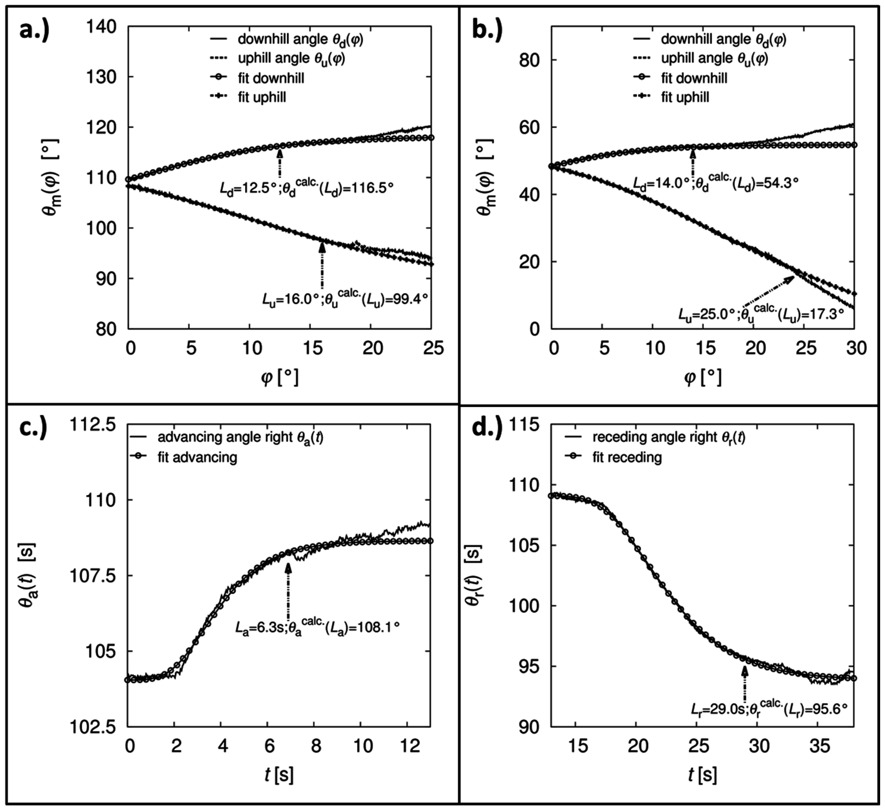
4.2. Static Contact Angle Analyses

A clear indication of the used notion of contact angles is important to avoid confusion. Due to the unknown local position of the triple line, all measured and calculated contact angles during contact angle analyses by drop shape detection are generally apparent contact angles (APCA). In this contribution, the notion “static” refers to the wetting situation without a moving contact line and should not be mixed up with the “as-placed” contact angle θAP [79]. The notion dynamic” in Section 4.3 and Section 4.4 also includes contact angles during the motion of the contact line. A common approach to characterize, e.g., pinning effects, coating quality, etc., is the determination of the contact angle hysteresis CAH by measuring the experimental available advancing θ a and receding θ r contact angles, which are essential static wetting characteristics. In literature, different procedures and definitions are used to obtain these angles. Generally, the identification of advancing and receding angles is performed by optical observation with the human eye and defining these angles depending on the triple line motion. The main problem of this procedure is that it depends of several criteria of the equipment (e.g., frame rate of video recording) and on the subjectivity of the operator. Different definitions for these angle are often used, e.g., “contact angle before, after or during the first observed triple line motion” from the same or different images. Unfortunately, these critical experimental conditions are rarely reported in literature resulting in poor comparability and reproducibility, especially for large CAH surfaces or surfaces with slip-stick behavior. To free this procedure from the subjectivity of the operator/optical observation and to enhance the comparability and reproducibility, the analysis procedures based on the data from HPDSA uses the coordinates of the triple points to identify advancing and receding angles. Due to the transformation in Cartesian coordinates and triple point detection (≡ chronologically first boundary points XB10), the shift of the boundary points ΔXB10 can be estimated, which corresponds to the covered distance of the triple line. The procedure is illustrated in Figure 5.
As illustrated in Figure 5, HPDSA leads to a subjective-free determination of static advancing and receding angles depending on the change of the triple point coordinates ΔXB10. This fact is especially interesting if more complicated surfaces are under investigation, e.g., such as slip-stick surfaces where multiple advancing θ d , e i and receding angles/motions θ u , e i depending on surface structure are observable (Figure 5c,d). The reproducible analysis of the motion behavior on such surfaces is quite a challenging task. However, due to the high sensitivity of the contact angle to the surface structure (a difference of few nm in roughness already changes the contact angle), this approach opens up the possibility to correlate the course of contact angles with local properties of the surface (roughness and/or heterogeneity) and to analyses the kinetics of the contact line dynamics, which was the main intention to develop the statistical contact angle analyses presented in Section 4.4.

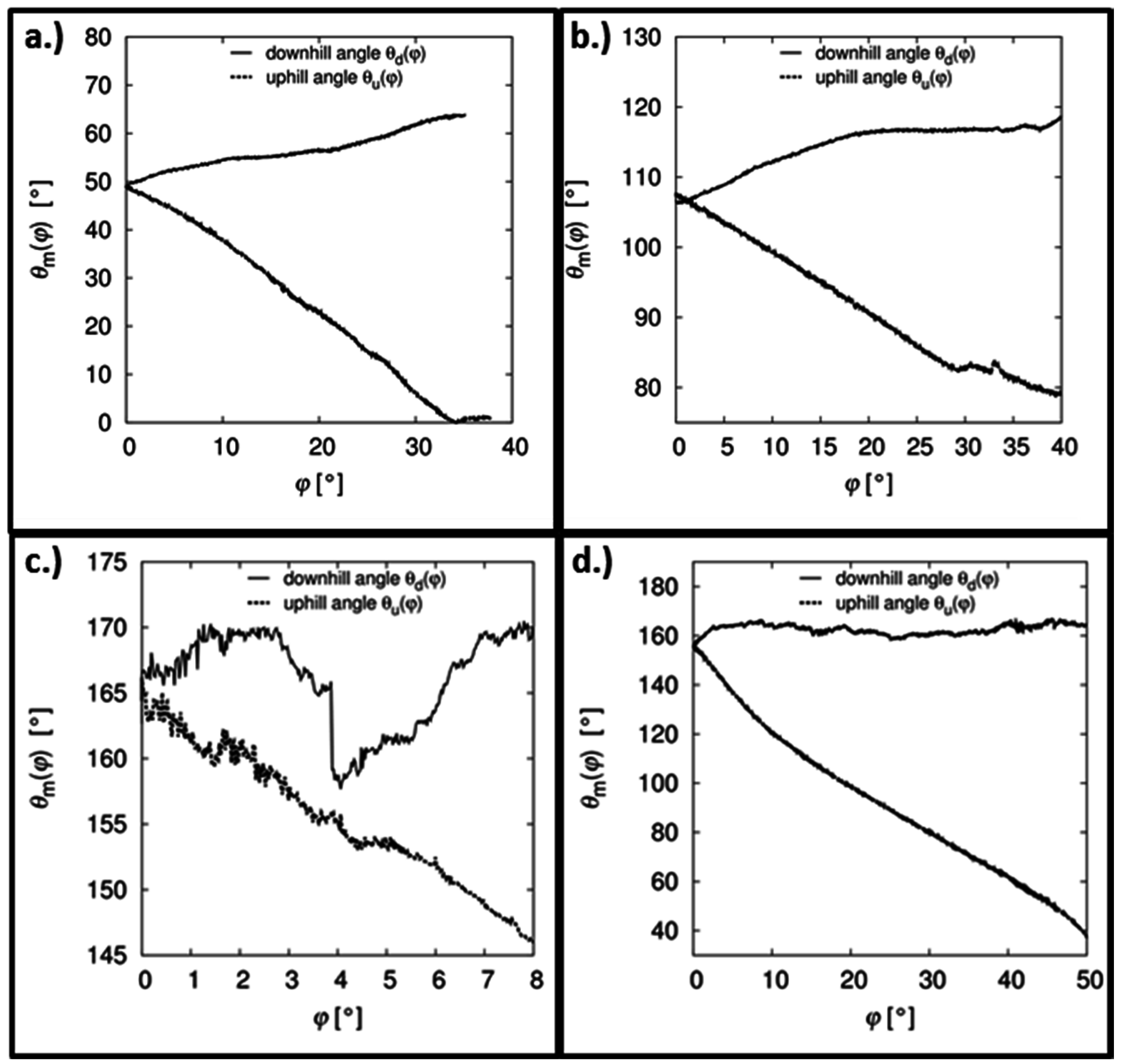
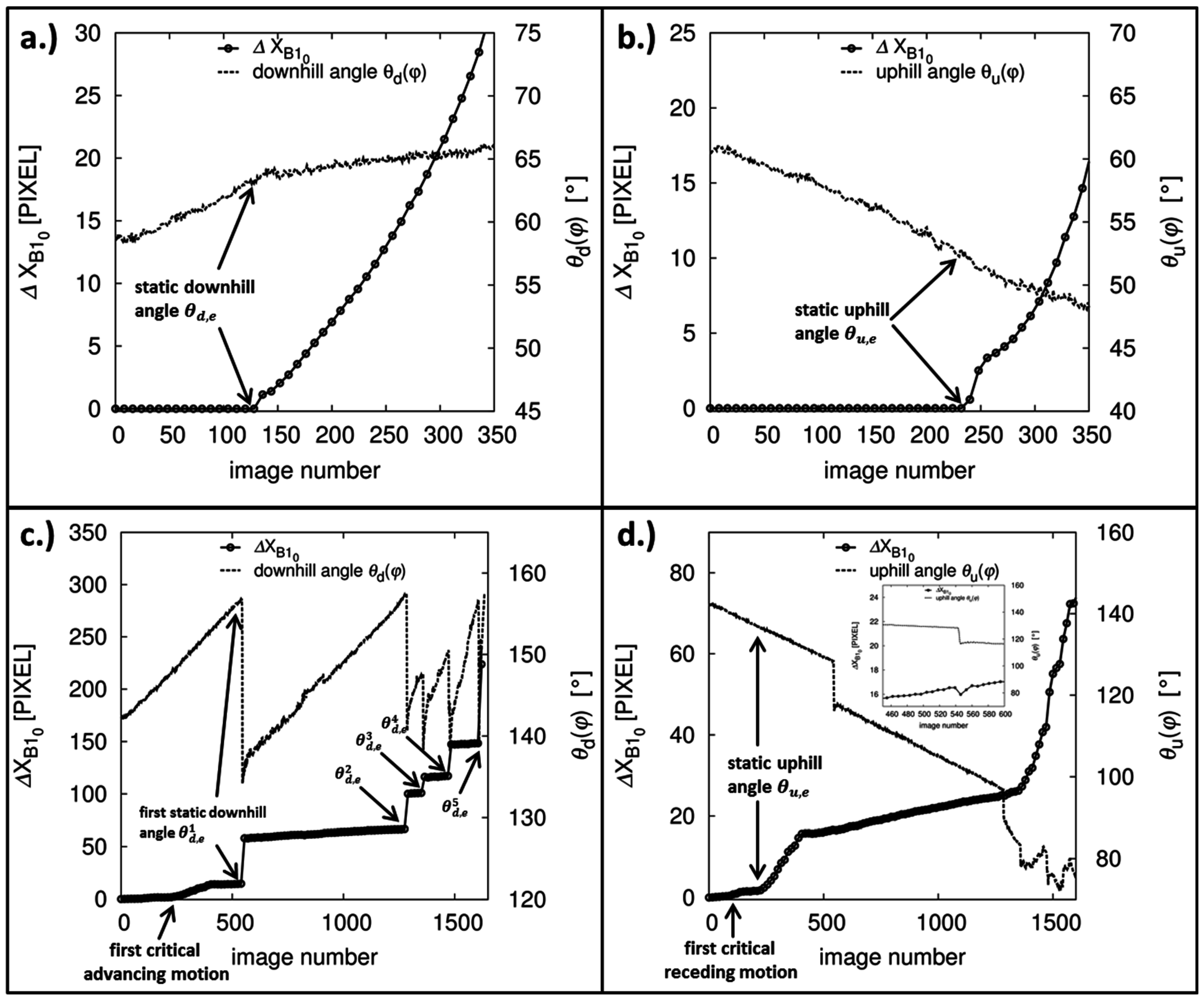
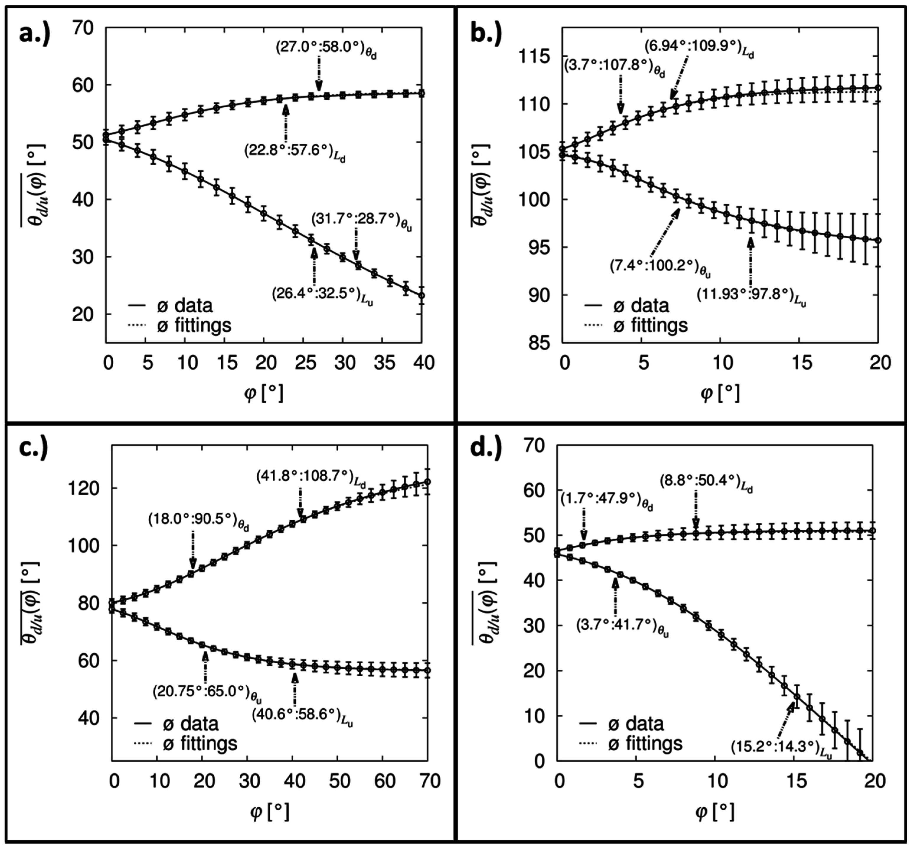
4.3. Dynamic Contact Angle Analyses: Individual and Overall Gompertzian Fitting Approach

The first step of the Gompertzian fitting approach is the fitting of a modified individual Gompertzian function onto the course of contact angles relative to a dependent parameter such as inclination angle φ (inclining-plate measurements) [71] or changing drop volume ΔV [72], respectively time t (horizontal-plate measurements) on an individual measuring position. The used Gompertzian functions are given by Equations (30)–(32),
f ( φ ) = θ m c a l c ( φ ) = θ s h i f t + A × exp [ exp ( k ( φ φ s h i f t ) ) ]
f ( Δ V ) = θ m c a l c ( Δ V ) = θ s h i f t + A × exp [ exp ( k ( Δ V Δ V s h i f t ) ) ]
f ( t ) = θ m c a l c ( t ) = θ s h i f t + A × exp [ exp ( k ( t t s h i f t ) ) ]
whereby θ s h i f t , A, k and φ s h i f t and ΔVshift or tshift, represent the fitting parameters and θ m c a l c is the contact angle calculated with the Gompertzian function in dependence on the inclination angle φ , change in drop volume ΔV or time t. Examples for Gompertzian fittings for inclining-plate and horizontal-plate measurements are illustrated in Figure 6.
The Gompertzian functions thereby simulate an “idealized steady course of contact angles relative to the dependent parameter without any unsteady behavior due to non-uniform pinning (e.g., slip-stick behavior, non-uniform slip behavior). The fitting limits for the downhill Ld and uphill Lu, respectively advancing La and receding Lr motion are manually definable and are generally defined at the point, when the motion transition from the slow-moving (triple line velocity 200   μ m / s ), which corresponds to a quasi-static wetting situation, to the high-velocity range (≡ macroscopic motion) is observed. In this range it can be assumed that the contact angles are almost independent of further parameters such as fluid dynamics and friction, resulting in significant differences from the idealized course of contact angles. To obtain more specific information about the wettability of a surface, the so-called Residual contact angles can be calculated by subtracting the individual Gompertzian function from the corresponding measured course of contact angles using Equations (33)–(35),
Δ θ d , u ( φ ) = θ d , u ( φ ) f ( φ ) = θ d , u ( φ ) θ d , u c a l c ( φ )
Δ θ a , r ( Δ V ) = θ a , r ( Δ V ) f ( Δ V ) = θ a , r ( Δ V ) θ a , r c a l c ( Δ V )
Δ θ a , r ( t ) = θ a , r ( t ) f ( t ) = θ a , r ( t ) θ a , r c a l c ( t )
whereas Equation (33) refers to the situation on an inclined-plate and Equations (34) and (35) refer to the situation on a horizontal plate depending on the chosen parameter ΔV of t. The corresponding Residual contact angles for the examples presented in Figure 6 are illustrated in Figure 7.
In the next step, the individual data are averaged, leading to averaged overall Gompertzian data, which can also be represented by an average Gompertzian function. This approach is effective to describe the evolution of dynamic contact angles with only one equation and a reduced set of parameters from a huge amount of contact angle data (between ≈ 10,000 and 35,000 considered contact angles per measurement series, resulting in four average parameters). Examples for averaged Gompertzian functions are illustrated in Figure 8.
The averaged data in Figure 8 describe the average behavior of liquid droplets on different positions on the surfaces during inclining-plate measurements, which strongly reduce the effect of the displacement of the droplets (the evaluation of horizontal measurements is also possible). It can be assumed that in an ideal case, an intersection point of all individual Gompertzian functions for all measuring positions should exist. On real surfaces, additional parameters such as surface roughness, heterogeneity, drop displacement, etc. lead to deviations from the “idealized behavior”. Therefore, to identify contact angles/ranges θ d / u with smallest standard deviations is reasonable to characterize the overall wettability of a surface.
Beside the identification of contact angle with lowest standard deviation, the overall curve shape analysis by Gompertzian fitting can be used to analyze the pinning and drain-off behavior of liquids on solid surfaces. In contrast to static contact angle analyses, the Gompertzian analyses also consider the quasi-static and dynamic movement of droplets during contact angle measurements. In particular, the fitting parameters A (amplitude of the contact angles ≡ difference between the theoretical smallest and largest contact angle) and k (rate constant of the data points) determine the course of the averaged Gompertzian function [80]. That means that weak pinning results in small amplitudes A and large slopes k, whereas strong pinning results in large amplitudes and small slopes of the data points. An example is illustrated in Figure 9. Note that the maximal slope/gradient of the Gompertzian function is proportional to k × A, which is reached if the exponential functions are one and 1/e, respectively. Hence, individual analyses of both parameters seem to be more reasonable but future investigations are in schedule.
The presented examples illustrate the plot of the k- and A-values against number of carbon atoms in the side chain of anionic fluorinated ionic liquids (black), cationic fluorinates ionic liquids (red) and non-fluorinated alkyl ionic liquids (blue), which were used as contact angle test liquids on different modified silicon surfaces [73,74]. Within the cited study, the pinning behavior of these liquids depending on the molecular structures was analyzed. Thereby, it was illustrated that the Gompertzian fitting approach is very effective to characterize these quantities and to classify solid–liquid combinations in terms of their A- and k-values, which are important parameters when, e.g., liquids or solid–liquid interface are involved in processes. In a recent study [75], this approach was used to investigate and analyze the wetting behavior on flat coated silicon wafers with different chemical surface textures. Thereby, it was illustrated that this approach might be useful to detect nano-heterogeneities (coating defects) and opens up to use contact angle measurements as a sensitive probe for surface characterization.

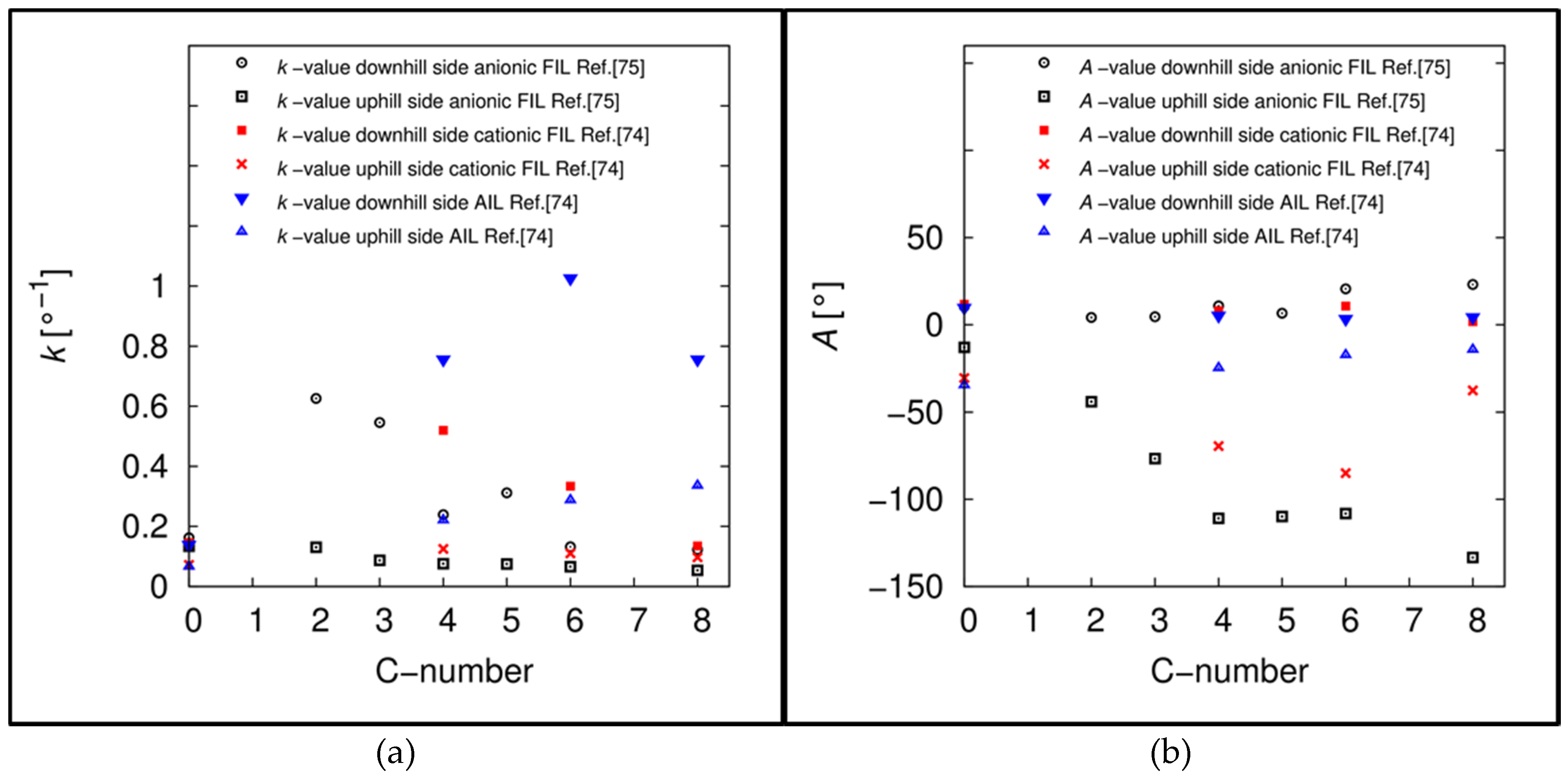
4.4. Statistical Contact Angle Analyses: Independent and Dependent Analyses

The statistical contact angle analyses [76,77,78] are based on the velocity determination of the triple line movement. The velocity or its change is normally used to define specific contact angles. Commonly performed analyses do not evaluate the whole range of the measurement but only determine one advancing and one receding angle as described in Section 4.2. Thus, we ask ourselves three questions: (1) “How is the reproducibility of determine just one advancing and one receding angle per measurement?” (2) “Why losing all the information about the surface, which is hidden in the triple line motion (acceleration/deceleration)?” (3) “Can the triple line motion be correlated with the microscopic surface structure?” On real surfaces (rough and/or heterogeneous), more than one triple line motion (acceleration/deceleration) can be observed due to the high sensitivity of the contact angle to the surface structure. In this regard, the first step of the analysis strategy is the determination of the triple line velocity using Equations (36)–(38),
( d x d φ ) No . = N o . 1 N o . + 1 ( x i φ i ) × 3 N o . 1 N o . + 1 ( φ i ) N o . 1 N o . + 1 ( φ i 2 ) × 3 ( N o . 1 N o . + 1 ( φ i ) ) 2
( d y d φ ) No . = N o . 1 N o . + 1 ( y i φ i ) × 3 N o . 1 N o . + 1 ( φ i ) N o . 1 N o . + 1 ( φ i 2 ) × 3 ( N o . 1 N o . + 1 ( φ i ) ) 2
where ( d x , d y / d φ ) No . are the rates of the x- and y-coordinates (No. = image number) obtained by three point linear regression of neighboring points. The total velocity of the triple points is the given as,
v e l ( φ ) No . = f × ( d x d φ ) No . 2 + ( d y d φ ) No . 2 × φ ˙
where φ ˙ is the inclination rate of the sample desk ( ° / s ) and f is +1 for downhill movement and −1 for uphill movement. To define the spectrum of contact angles that will be considered, the contact angles are classified by two conditions: contact angles during a constant velocity (zero or limited) and contact angles during an acceleration/deceleration event. In the second case, the angles are defined before, during and after the acceleration/deceleration, which corresponds to common definitions for specific contact angles. Thereby, the contact angle data for every measuring position are considered as independent random experiments. To identify the contact angle events, the change of the triple line velocity between two neighboring images is calculated by Equation (39),
Δ v e l No . / No . ± 1 = ± [ v e l ( φ ) No . ± 1 v e l ( φ ) No . ]
which has to be larger than a definable limit value lv. This procedure is integrated in an automatic processing routine, which uses the conditions in Table 2 for the automatic read-out.
The core of the statistical analyses is a counting and calculation algorithm of the obtained contact angle events. The four investigated parameters p for every event are the inclination angle φ , the contact angle θ , the velocity of the triple point vel and the covered distance of the triple point relative to the chronological first triple point dis. As a practical tip, it is recommended to restrict the upper-limit to the slow-moving range (quasi-static wetting situation), which is less affected by flow dynamics, see Figure 10.
During the Independent statistical analysis, independent expectation values and standard deviations of the former obtained contact angle events were calculated using Equations (40) and (41),
E ( p ) = n = 1 i p i n
σ ( p ) = n = 1 i [ ( n 1 ) 1 × ( p i E ( p ) ) 2 ]
with n the number of considered events leading to the so-called “global values” for every investigated parameter. An example for the independent statistical contact angle analysis on a flat hydrophobic modified silicon wafer is illustrated in Table 3 [78].
In the cited study [78], the wetting behavior on a flat hydrophobic modified and on a defined rough ( R a 20   nm ;   R q 26   nm ) silicon wafer were investigated and compared. Thereby, ten inclining-plate measurements per surface were performed resulting in overall ≈ more than 18,000 considered contact angels for the statistical analyses. As illustrated in Table 3, the automatic read-out resulted in a large number for every considered contact angle events. This example illustrates that the determination of only one specific contact angle pair is insufficient and neither reliable nor reproducible. Because the determination of just one advancing and receding contact angle strongly depends on factors such as frame rate of the video recording, resolution in time and space, etc. In contrast, the independent contact angle analysis illustrates that there exists a relative large range of advancing and receding angles ( σ (advancing) ≈ 3.5°; σ (receding) ≈ 7.5°) even on a “simple” surface (flat, hydrophobic modified) so that the commonly performed procedures do identify advancing and receding angles does not lead to a sufficient statistical accuracy. If the correlation between the different parameters p is taken into account, the investigation of contact angle distributions in more detail is possible. This approach is called “dependent statistical contact angle analysis”. In a first step, the former obtained contact angle events were allocated into classes relative to the standard deviation of the independent analysis. The class size can be manually defined but was in general between σ(p) × 0.125 and σ(p) × 0.5. The counting of every value within the classes leads to density distributions relative independent parameter, which can be presented in histograms as illustrated in Figure 11. Overall, this approach is able to investigate 96 distributions for every event, Table 2.
As explained within the cited study [78] and illustrated in Figure 11, this approach has a fine local resolution and is especially reasonable to analyze the different wetting behavior with regard to different microscopic surface topographies. The physical and chemical heterogeneity of a surface is the main reason for the pinning of the triple line which induces the acceleration/deceleration motions during a dynamic measurement. To analyze these motions and their dependencies in detail, expectation values and standard deviations for the inclination angle φ, the contact angle θ, the triple line velocity vel and the covered distance relative to the first intersection point dis can be calculated. Depending on the parameter that is investigated, this approach results in density distributions which are specific for the investigated surface. As demonstrated, within the cited study [78] the density distributions on the patterned surface are monomodal and symmetric with smaller velocities and covered distances of the acceleration events in comparison to the monomodal asymmetric distributions with larger velocities and covered distances of the flat coated silicon surface coated with the same siloxane. Hence, it is possible to analyze surface properties with high resolution and to correlate the motion behavior of liquid drops with the local properties of the surface.

5. Summary

Static and dynamic wetting behaviors of liquid droplets on solid surfaces are strongly influenced by the physical and chemical properties resulting in a range of possible apparent and equilibrium contact angles. Thus, the meaningful analysis and interpretation of contact angle measurements still remain a challenging task and is less simple than it had appeared to be. Beside some experimental influence quantities such as drop displacement, drop volume, horizontal or inclined set-up, etc., contact angle determination also depends on the image analysis and the used fitting procedure to extract the contact angle from the experimental drop shape. Due to the generally non-axisymmetric drop profiles on real surfaces, commercial analyses strategies such as ellipse-fitting, circle-fitting or tangent-fitting approaches, which mostly consider the whole drop shape, result in large inaccuracies, especially for extreme wetting situations such as low contact angle surfaces, superhydrophobic and rose petal surfaces, which might lead in the worst case even in misinterpretations and misleading concepts presented in the scientific literature. The developed high-precision drop shape analysis (HPDSA) procedure (HPDSA and statistical analyses) is a concept to enhance the reproducibility of contact angle analysis and to free the procedure from several subjective criteria of the operator. Therefore, drop images are transformed to Cartesian coordinates, which opens up to use every meaningful physical and mathematical approach. According to the Laplace equation, a circular function for the left-hand and right-hand side of the drop shape is used for the fitting algorithm, where only the region near the three phase interphase (≡ often called triple point) is considered resulting in a high-precision contact angle calculation. Furthermore, the triple points can be detected and the baseline can be dynamically monitored so that moving baselines are analyzable. In this regard, static wetting properties (advancing and receding angles) can be identified on a mathematical base instead of optical observation with human eye. Simple, static analysis without discretization was demonstrated but because contact angles are very sensitive to surface properties and “starting conditions”, three analysis strategies, which are the individual and overall Gompertzian fitting, the independent statistical contact angle analysis and the dependent statistical contact angle analysis, were developed to analyze contact angle measurements more in detail. The Gompertzian fitting approaches are based on the fitting of a modified sigmoid function onto the course of contact angles relative to a dependent parameter such as inclination angle, drop volume or time. This function is very effective to describe the progression of contact angles and can be used for Residual/Individual analysis by subtraction of the fit function from the measured course of contact angles. Then, the surface wettability can be analyzed with a fine local resolution. Averaging of the individual Gompertzian functions lead to the overall Gompertzian function, which is able to describe the overall wettability from a huge amount of contact angle data (≈10,000 to 35,000 considered contact angles per measurement) with only four fitting parameters. By calculating standard deviations, contact angles and contact angle ranges with lowest standard deviation can be identified, which are statistical robust and characteristic quantities for the overall wettability of the surface. Furthermore, the fitting parameters k and A, which determine the course of the Gompertzian function, can be used to characterize the “uniform” pinning (or hysteresis) behavior of a liquid droplet onto a surface. The independent and dependent statistical contact angle analyses are based on the determination of the change of triple line velocity and the automatic read out of contact angle events depending on the velocity change. Due to aspects like local heterogeneities on real surfaces, more than one advancing and receding contact angle can be observed during the slip-stick motion of the triple line depending on the degree of roughness and heterogeneity. On the one hand, the statistical approaches lead to the “global-values”, which are statistically reproducible expectation values. On the other hand, the contact angle behavior can be correlated with local surface properties on the few-nanometer scale because the hysteresis is a sensitive tool for detecting heterogeneities of surface. Hence, contact angle measurements using droplets with base diameters more than 5 mm can even be used as a sensitive probe like for detecting differences in the structure of 20 nm in height [78]. At this point it should be noted that the presented analyses strategies are not restricted to the high-precision drop shape analysis calculation. In addition, contact angle data obtained from commercial analysis equipment can be used but generally with reduced sensitivity. Using these approaches lead, in our opinion, to contact angle data with enhanced reproducibility and help to avoid misinterpretations of wetting experiments. In this regard, we want to encourage not just the small community of specialists but especially the multiple users of sessile drop experiments to perform meaningful contact angle measurements and analyses instead of just measuring some angles in-between the advancing and receding angle. Especially, naming and storing of the experimental conditions such as drop volume, inclination rate, vapor atmosphere, contact angle definition, frame rate, etc., as illustrated in our investigations [53,54,64,71,72,73,74,75,76,77,78], are mandatory to ensure reproducibility and comparability of sessile drop experiments.

Acknowledgments

We want to thank Wulff Possart for his scientific guidance and especially for his perfect lessons, which led us deeper into the topic of surface analysis. Furthermore, we want to thank Rolf Hempelmann, Daniel Rauber (experimental support concerning ionic liquids), Sven Ingebrandt and Walid-Madhat Munief (preparation and surface modification), Dan Durneata (assistance and programming), Katja Groß and Julia Grub (experimental support), Rudolf Richter, Jens Wiegert and Norbert Ochs (mechanical workshop).

Author Contributions

Florian Heib conceived, designed and performed the wetting experiments, analyzed the data and wrote the paper. Michael Schmitt contributed equally to the manuscript, supported the data analysis, did the programming of the HPDSA routine and corrected the paper.

Conflicts of Interest

The authors declare no conflict of interest.

Abbreviations

The following abbreviations are used in this manuscript:
α B L Inclination angle of the baseline
Γ D Absolute adsorption
γ l , v Interfacial tension between the liquid and vapor interfaces
γ s , l Interfacial tension between the solid and liquid interfaces
γ s , v g Y o u n g Interfacial tension between the solid and liquid interface according to the generalized Young equation
γ s , v Y o u n g Interfacial tension between the solid and liquid interface according to the Young equation
Δ θ Contact angle hysteresis
Δ θ a ( φ ) 
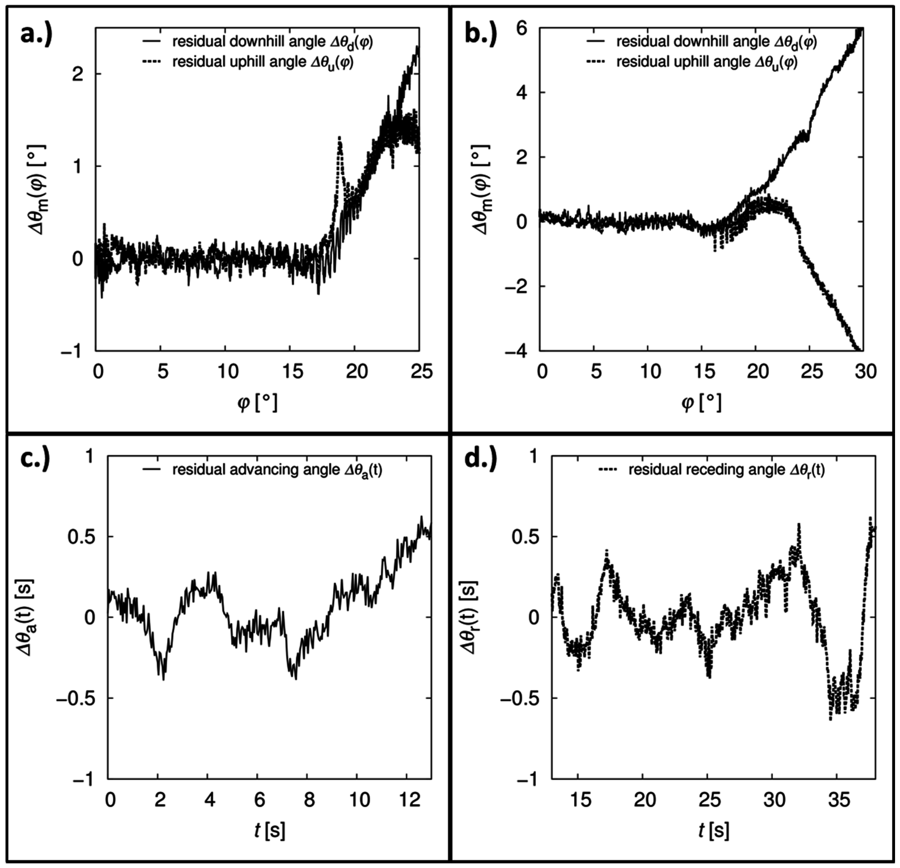
Residual advancing angle depending on the inclination angle
Δ θ a ( t ) Residual advancing angle depending on the time
Δ θ a ( Δ V ) Residual advancing angle depending on the change of drop volume
Δ θ d ( φ ) Residual downhill angle depending on the inclination angle
Δ θ d ( t ) Residual downhill angle depending on the time
Δ θ d ( Δ V ) Residual downhill angle depending on the change of drop volume
Δ θ r ( φ ) Residual receding angle depending on the inclination angle
Δ θ r ( t ) Residual receding angle depending on the time
Δ θ r ( Δ V ) Residual receding angle depending on the change of drop volume
Δ θ u ( φ ) Residual uphill angle depending on the inclination angle
Δ θ u ( t ) Residual uphill angle depending on the time
Δ θ u ( Δ V ) Residual uphill angle depending on the change of drop volume
Δ F Difference in forces
Δ p g L Difference in pressure between the convex and concave side of an interface according to the generalized Young–Laplace equation
Δ p L a p l a c e Difference in pressure between the convex and concave side of an interface according to the Young–Laplace equation
Δ V Change of drop volume during contact angle measurements
Δ V s h i f t Fitting parameter of the Gompertzian function
Δ v e l No . / No . ± 1 Change of triple line velocity between two neighboring images
Δ X B 10 Shift of the boundary/triple points
Δ y Difference in height coordinates between the triple points and center of the fitting circle
θ a Advancing contact angle
θ A P As-placed contact angle
θ C B Cassie–Baxter contact angle
θ d Downhill contact angle during inclining-plate experiments
θ d , e Static downhill angle
θ d / u Downhill and uphill angles with lowest standard deviation
θ m Measured/apparent contact angle
θ m c a l c . ( φ ) Contact angle calculated with a Gompertzian function depending on the inclination angle
θ m c a l c . ( t ) Contact angle calculated with a Gompertzian function depending on the time
θ m c a l c . ( Δ V ) Contact angle calculated with a Gompertzian function depending on the change of drop volume
θ r Receding contact angle
θ s h i f t Fitting parameter of the Gompertzian function
θ u Uphill angle during inclining-plate experiments
θ u , e Static uphill angle
θ W Wenzel contact angle
θ Y Equilibrium/Young contact angle
κ s , l , v Three phase interfacial tension/line tension
λ i j Gravitational corrected chemical potential of component i in the phase j
μ i j Chemical potential of component i in the phase j
σ ( p ) Standard deviation of the chosen parameter p
σ ( x ) Standard deviation of color rate weighted expectation value in x-direction
σ ( y ) Standard deviation of color rate weighted expectation value in y-direction
φ Inclination angle of the sample desk during inclining-plate measurements
φ ˙ Inclination rate of the sample desk
φ s Angle between the substrate surface and the local principal plane of the three phase contact line
φ s h i f t Fitting parameter of the Gompertzian function
ϕ Angle relative to the gravitational field
A Area
A Fitting parameter of the Gompertzian function
A a Slope of the linear regression for the advancing angle
A g e o Geometrically modeled surface area
A r Slope of the linear regression for the receding angle
A r e a l Real surface area
ADSAAxisymmetric drop shape analysis
APCAApparent contact angle
APSMono-aminopropylsiloxane
b a r c Real length of an calculation arc
c i Curvature constants
CAHContact angle hysteresis
c o l Sum of color values for one pixel
d a r c Minimal length of an calculation arc
d i s Covered distance of the triple point
E ( p ) Expectation value of the chosen parameter p
E ( x ) Color rate weighted expectation value in x-direction
E ( y ) Color rate weighted expectation value in y-direction
FCFFast circle fit
f Fraction of the solid surface wetted by the liquid
g Gravity acceleration
HPDSAHigh-precision drop shape analysis
k Fitting parameter of the Gompertzian function
L a Fitting limit of the Gompertzian function for the advancing motion
L d Fitting limit of the Gompertzian function for the advancing/downhill motion
L u Fitting limit of the Gompertzian function for the receding/uphill motion
L r Fitting limit of the Gompertzian function for the receding motion
l v Limit value
M i Molar mass of the component i
p Rate of color value for every pixel
p x i Rate of color value in x-direction
p y i Rate of color value in y-direction
R i Principle radii of curvature
R x Radius of an ellipse in x-direction
R y Radius of an ellipse in y-direction
r A Specific factor in the Tadmor equation for the advancing angle
r R Specific factor in the Tadmor equation for the receding angle
r f Roughness ration in the Cassie–Baxter equation
r w Roughness ratio in the Wenzel equation
t s h i f t Fitting parameter of the Gompertzian function
v e l ( φ ) No . Velocity of the triple line
w i ( x ) Influencing factors for noise correction
x B i x-Coordinate of the boundary/triple points
x C C x-Coordinate of the center of a fitting circle
x E C x-Coordinate of the center point of an ellipse
x M P x-Coordinate of the center of a fitting circle
x T P x-Coordinate of the triple point
y B i y-Coordinate of the boundary/triple points
y C C y-Coordinate of the center of a fitting circle
y E C y-Coordinate of the center point of an ellipse
y M P y-Coordinate of the center of a fitting circle
y T P y-Coordinate of the triple point
z Elevation in the gravitational field

References

  1. Wang, X.; Chen, L.; Bonaccurso, E.; Venzmer, J. Dynamic wetting of hydrophobic polymers by aqueous surfactant and superspreader solutions. Langmuir 2013, 29, 14855–14864. [Google Scholar] [CrossRef] [PubMed]
  2. Tonooka, K.; Kikuchi, N. Super-hydrophilic and solar-heat-reflective coatings for smart windows. Thin Solid Films 2013, 532, 147–150. [Google Scholar] [CrossRef]
  3. Bormashenko, E.; Stein, T.; Whyman, G.; Pogreb, R.; Sutovsky, S.; Danoch, Y.; Shoham, Y.; Bormashenko, Y.; Sorokov, B.; Auerbach, D. Superhydrophobic metallic surfaces and their wetting properties. J. Adhes. Sci. Technol. 2008, 22, 379–385. [Google Scholar] [CrossRef]
  4. Marmur, A. Solid-surface characterization by wetting. Annu. Rev. Mater. 2009, 39, 473–489. [Google Scholar] [CrossRef]
  5. Kamusewitz, H.; Possart, W. The Thermodynamics and wetting of real surfaces and their relationship to adhesion. Int. J. Adhes. Adhes. 1993, 13, 77–84. [Google Scholar]
  6. Good, R.J. Contac-Angle, Wetting, and adhesion—A critical review. J. Adhes. Sci. Technol. 1993, 6, 1269–1302. [Google Scholar] [CrossRef]
  7. Amirfazli, A. Interpretation of contact angle data to estimate drop adhesion onto solid surfaces. Am. Chem. Soc. 2010, 240, 1155. [Google Scholar]
  8. Wu, J.B.; Zhang, M.Y.; Wang, X.; Li, S.B.; Wen, W.J. A simple approach for local contact angle determination on a heterogeneous surface. Langmuir 2011, 27, 5705–5708. [Google Scholar] [CrossRef] [PubMed]
  9. Ryan, B.J.; Poduska, K.M. Roughness effects on contact angle measurements. Am. J. Phys. 2008, 76, 1074–1077. [Google Scholar] [CrossRef] [Green Version]
  10. Giljean, S.; Bigrelle, M.; Anselme, K.; Haidara, H. New insights on contact/roughness dependence on high surface energy materials. Appl. Surf. Sci. 2011, 257, 9631–9638. [Google Scholar] [CrossRef]
  11. Marmur, A. Superhydrophobic and superhygrophobic surfaces: From understanding non-wettability to design considerations. Soft Matter 2013, 9, 7900–7904. [Google Scholar] [CrossRef]
  12. Krumpfer, J.W.; Bian, P.; Zheng, P.W.; Gao, L.C.; McCarthy, T.J. Contact angle hysteresis on superhydrophobic surfaces: An ionic liquid probe fluid offers mechanistic insights. Langmuir 2011, 27, 2166–2169. [Google Scholar] [CrossRef] [PubMed]
  13. Yan, Y.Y.; Gao, N.; Barthlott, W. Mimicking natural superhydrophobic surfaces and grasping the wetting process: A review on recent progress in preparing superhydrophobic surfaces. Adv. Colloid Interface Sci. 2011, 169, 80–105. [Google Scholar] [CrossRef] [PubMed]
  14. Bormashenko, E.; Grynyov, R.; Chaniel, G.; Taitelbaum, H.; Bormashenko, Y. Robust technique allowing manufacturing superolephobic surfaces. Appl. Surf. Sci. 2013, 270, 98–103. [Google Scholar] [CrossRef]
  15. Grynyov, R.; Bormashenko, E.; Whyman, G.; Bormashenko, Y.; Musin, A.; Pogreb, R.; Starostin, A.; Valtsifer, V.; Strlnikov, V.; Schechter, A.; et al. Superoleophobic surfaces obtained via hierarchical metallic meshes. Langmuir 2016, 32, 4134–4140. [Google Scholar] [CrossRef] [PubMed]
  16. Whyman, G.; Bormashenko, E. Wetting Transitions on Rough Substrates: General Considerations. J. Adhes. Sci. Technol. 2012, 26, 207–220. [Google Scholar]
  17. Bormashenko, E.; Musin, A.; Whyman, G.; Zinigrad, M. Wetting transitions and depinning of the triple line. Langmuir 2012, 28, 3460–3464. [Google Scholar] [CrossRef] [PubMed]
  18. Bormashenko, E.Y. Wetting of Real Surfaces; deGryter Verlag: Berlin, Germany, 2013. [Google Scholar]
  19. Kamusewitz, H.; Possart, W.; Paul, D. Measurements of solid-water contact angles in the presence of different vapors. Int. J. Adhes. Adhes. 1993, 13, 143–149. [Google Scholar] [CrossRef]
  20. Kwok, D.Y.; Neumann, A.W. Contact angle measurements and contact angle interpretation. Adv. Colloid Interface Sci. 1999, 81, 167–249. [Google Scholar] [CrossRef]
  21. De Gennes, P.-G.; Brochart-Wyart, F.; Quéré, D. Capillarity and Wetting Phenomena: Drops, Bubbles, Pearls, Waves; Springer: Berlin, Germany, 2004. [Google Scholar]
  22. Erbil, H.Y. Surface Chemistry of Solid and Liquid Interfaces; Blackwell Publishing Ltd.: Malden, MA, USA, 2006. [Google Scholar]
  23. Kwok, D.Y.; Gietzelt, T.; Grundke, K.; Jacobasch, H.J.; Neumann, A.W. Contact angle measurements and contact angle interpretation: 1. Contact angle measurements by axisymmetric drop shape analysis and a goniometer sessile drop technique. Langmuir 1997, 13, 2880–2894. [Google Scholar] [CrossRef]
  24. Marmur, A. Hydro- hygro- oleo- omnio-phobic? Terminology of wettability classification. Soft Matter 2012, 8, 6867–6870. [Google Scholar] [CrossRef]
  25. Young, T. An essay on the Cohesion of Fluids. Philos. Trans. Royal Soc. Lond. 1805, 95, 65–87. [Google Scholar] [CrossRef]
  26. Laplace, P.S. Méchanique Céleste. Available online: https://archive.org/details/mcaniquecles03lapl (accessed on 31 October 2016).
  27. Gibbs, G.W. On the equilibrium of heterogeneous substances. Am. J. Sci. 1878, 3, 441–458. [Google Scholar] [CrossRef]
  28. Rusanov, A.I. Surface thermodynamics revisited. Surf. Sci. Rep. 2005, 58, 111–239. [Google Scholar] [CrossRef]
  29. Rusanov, A.I. Thermodynamics of solid surfaces. Surf. Sci. Rep. 1996, 23, 173–247. [Google Scholar] [CrossRef]
  30. Ward, C.A.; Sasges, M.R. Effect of gravity on contact angle: A theoretical investigation. J. Chem. Phys. 1998, 109, 3651–3660. [Google Scholar] [CrossRef]
  31. Sasges, M.R.; Ward, C.A. Effect of gravity on contact angle: An experimental investigation. J. Chem. Phys. 1998, 109, 3661–3670. [Google Scholar] [CrossRef]
  32. Fuji, H.; Nakae, H. Effect of gravity on contact angle. Philos. Mag. A 1995, 72, 1505–1512. [Google Scholar] [CrossRef]
  33. Ward, C.A.; Rahimi, P.; Sasges, M.R.; Stanga, D. Contact angle hysteresis generated by the residual gravitational field of the Space Shuttle. J. Chem. Phys. 2000, 112, 7195–7202. [Google Scholar] [CrossRef]
  34. Voltcu, O.; Elliot, A.W. Equilibrium of multi-phase systems in gravitational fields. J. Phys. Chem. B 2008, 112, 11981–11989. [Google Scholar]
  35. Blokhuis, E.M.; Shikrot, Y.; Widom, B. Young’s law with gravity. Mol. Phys. 1995, 86, 891–899. [Google Scholar] [CrossRef]
  36. Brutin, D.; Zhu, Z.Q.; Rahli, O.; Xie, J.C.; Liu, Q.S.; Tadrist, L. Sessile drop in microgravity: Creation, Contact angle and interface. Microgravity Sci. Technol. 2009, 21, 67–76. [Google Scholar] [CrossRef]
  37. Marmur, A. Measures of wettability of solid surface. Eur. Phys. J. Spec. Top. 2011, 197, 193–198. [Google Scholar] [CrossRef]
  38. Shanahan, M.E.R.; Di Meglio, J.M. Wetting hysteresis: Effects due to shadowing. J. Adhes. Sci. Technol. 1994, 8, 1371–1380. [Google Scholar] [CrossRef]
  39. Bormashenko, E.; Bormashenko, Y.; Whyman, G.; Pogreb, R.; Musin, A.; Jager, R.; Barkay, Z. Contact angle hysteresis on polymer substrates established with various experimental techniques, its interpretation, and quantitative characterization. Langmuir 2008, 24, 4020–4025. [Google Scholar] [CrossRef] [PubMed]
  40. Grundke, K.; Poschel, K.; Synytska, A.; Frenzel, R.; Drechsler, A.; Nitschke, M.; Cordeiro, A.L.; Uhlmann, P.; Welzel, P.B. Experimental studies of contact angle hysteresis phenomena on polymer surfaces—Toward the understanding and control of wettability for different applications. Adv. Colloid Interface Sci. 2015, 222, 350–376. [Google Scholar] [CrossRef] [PubMed]
  41. Starov, V. Static contact angle hysteresis on smooth, homogeneous solid substrates. Colloid Polym. Sci. 2013, 291, 261–270. [Google Scholar] [CrossRef]
  42. Wenzel, R.N. Resistance of solid surfaces to wetting by water. Ind. Eng. Chem. 1936, 28, 988–994. [Google Scholar] [CrossRef]
  43. Cassie, A.B.D.; Baxter, S. Wettability of porous surfaces. Trans. Faraday Soc. 1944, 40, 546–551. [Google Scholar] [CrossRef]
  44. Bormashenko, E. Progress in understanding wetting transitions on rough surfaces. Adv. Colloid Interface Sci. 2015, 222, 92–103. [Google Scholar] [CrossRef] [PubMed]
  45. David, R.; Neumann, W.A. Energy barriers between the Cassie and Wenzel wetting states on random superhydrophobic surfaces. Colloids Surf. A 2013, 425, 51–58. [Google Scholar] [CrossRef]
  46. Tadmor, R. Line energy and the relation between advancing, receding and Young contact angles. Langmuir 2004, 20, 7659–7664. [Google Scholar] [CrossRef] [PubMed]
  47. Schulze, R.-D.; Possart, W.; Kamusewitz, H.; Bischof, C. Young’s equilibrium contact angle on rough solid surfaces. Part I. An empirical determination. J. Adhes. Sci. Technol. 1989, 3, 39–48. [Google Scholar] [CrossRef]
  48. Kamusewitz, H.; Possart, W. Wetting and scanning force microscopy on rough polymer surfaces: Wenzel’s roughness factor and the thermodynamic contact angle. Appl. Phys. A 2003, 76, 899–902. [Google Scholar]
  49. Joanny, J.F.; De Gennes, P.G. Model for contact angle hysteresis. J. Chem. Phys. 1984, 81, 552–562. [Google Scholar] [CrossRef]
  50. Shanahan, M.E.R. Effect of surface flaws on the wettability of solids. J. Adhes. Sci. Technol. 1992, 6, 489–501. [Google Scholar] [CrossRef]
  51. Marmur, A. Soft contact: Measurements and interpretation of contact angle. Soft Matter 2006, 2, 12–17. [Google Scholar] [CrossRef]
  52. Bittoun, E.; Marmur, A. Chemical nano-heterogeneities detection by contact angle hysteresis: Theoretical feasibility. Langmuir 2010, 25, 1277–1281. [Google Scholar] [CrossRef] [PubMed]
  53. Schmitt, M.; Hempelmann, R.; Heib, F. Experimental Investigation of dynamic contact angles on horizontal and inclined surfaces part I: Flat silicon oxide surfaces. Z. Phys. Chem. 2014, 228, 11–25. [Google Scholar] [CrossRef]
  54. Schmitt, M.; Hempelmann, R.; Heib, F. Experimental Investigation of dynamic contact angles on horizontal and inclined surfaces part II: Rough homogeneous surfaces. Z. Phys. Chem. 2014, 228, 629–648. [Google Scholar] [CrossRef]
  55. Krasovitski, B.; Marmur, A. Drops down the hill: Theoretical study of limiting contact angles and the hysteresis range on a tilted plate. Langmuir 2005, 21, 3881–3885. [Google Scholar] [CrossRef] [PubMed]
  56. Tadmor, R.; Chaurasia, K.; Yadav, P.S.; Leh, A.; Bahadur, P.; Dang, L.; Hoffer, W.R. Drop retention force as a function of resting time. Langmuir 2008, 24, 9370–9374. [Google Scholar] [CrossRef] [PubMed]
  57. Yadav, P.S.; Bahadur, P.; Tadmor, R.; Chaurasia, K.; Leh, A. Drop retention force as a function of drop size. Langmuir 2008, 24, 3181–3184. [Google Scholar] [CrossRef] [PubMed]
  58. Del Rio, O.I.; Kwok, D.Y.; Wu, R.; Alvarez, J.M.; Neuman, A.W. Contact angle measurements by axisymmetric drop shape analysis and an automated polynomial program. Colloids Surf. A 1998, 143, 197–210. [Google Scholar] [CrossRef]
  59. Kalantarian, A.; David, R.; Neumann, A.W. Methodology for high accuracy contact angle measurement. Langmuir 2009, 25, 14146–14154. [Google Scholar] [CrossRef] [PubMed]
  60. Kalantarian, A.; David, R.; Chen, J.; Neumann, A.W. Simultaneous measurement of contact angle and surface tension using axisymmetric drop-shape analysis-no apex (ADSA-NA). Langmuir 2011, 27, 3485–3495. [Google Scholar] [CrossRef] [PubMed]
  61. Emelyanenko, A.M.; Boinovich, L.B. The role of discretization in video image processing of sessile and pendant drop profiles. Colloids Surf. A 2001, 189, 197–202. [Google Scholar] [CrossRef]
  62. Biole, D.; Wang, M.; Bertola, V. Assessment of direct image processing methods to measure the apparent contact angle of liquid drops. Exp. Therm. Fluid Sci. 2016, 76, 296–305. [Google Scholar] [CrossRef]
  63. Volpe, D.C.; Siboni, S. Use, abuse, misuse and proper use of contact angles: A critical review. Rev. Adhes. Adhes. 2015, 3, 365–385. [Google Scholar] [CrossRef]
  64. Schmitt, M.; Heib, F. High-precision drop shape analysis on inclining flat surfaces: Introduction and comparison of this special method with commercial contact angle analysis. J. Chem. Phys. 2013, 139, 134201. [Google Scholar] [CrossRef] [PubMed]
  65. Tadmor, R.; Bahadur, P.; Leh, A.; N’guessan, H.E.; Jaini, R.; Dang, L. Measurement of lateral adhesion forces at the interface between a liquid drop and a substrate. Phys. Rev. Lett. 2009, 103, 266101. [Google Scholar] [CrossRef] [PubMed]
  66. N’guessan, H.E.; Leh, A.; Cox, P.; Bahadur, P.; Tadmor, R.; Patra, P.; Vajtai, R.; Ajayan, P.M.; Wasnik, P. Water tribology on graphene. Nat. Commun. 2012, 3, 1242. [Google Scholar] [CrossRef] [PubMed]
  67. Tadmor, R. Misconceptions in wetting phenomena. Langmuir 2013, 29, 15474–15475. [Google Scholar] [CrossRef] [PubMed]
  68. Leh, A.; N’guessan, H.E.; Fan, J.; Bahadur, P.; Tadmor, R.; Zhao, Y. On the role of the three-phase contact line in surface deformation. Langmuir 2012, 28, 5795–5801. [Google Scholar] [CrossRef] [PubMed]
  69. Tadmor, R. Drops that pull themselves up. Surf. Sci. 2014, 628, 17–20. [Google Scholar] [CrossRef]
  70. Schmitt, M.; Hempelmann, R.; Groß, K.; Heib, F. Introduction in the high-precision drop shape analysis (HPDSA). In Proceedings of the European Adhesion Conference (EURADH), Alicante, Spain, 22–25 April 2014.
  71. Schmitt, M.; Hempelmann, R.; Ingebrandt, S.; Munief, W.-M.; Groß, K.; Grub, J.; Heib, F. Statistical contact angle analyses: “Slow moving” drops on inclining flat mono-aminopropylsiloxane surfaces. J. Adhes. Sci. Technol. 2015, 29, 1796–1806. [Google Scholar] [CrossRef]
  72. Schmitt, M.; Grub, J.; Heib, F. Statistical contact angle analyses; “slow moving” drops on a horizontal silicon-oxide surface. J. Colloid Interface Sci. 2015, 447, 248–253. [Google Scholar] [CrossRef] [PubMed]
  73. Rauber, D.; Heib, F.; Schmitt, M.; Hempelmann, R. Influence of perfluoroalkyl-chains on the surface properties of 1-methylimidazolium bis(trifluoromethanesulfonyl imide ionic liquids. J. Mol. Liq. 2016, 216, 246–258. [Google Scholar] [CrossRef]
  74. Heib, F.; Rauber, D.; Dier, T.; Volmer, D.A.; Hempelmann, R.; Schmitt, M. On the physicochemical and surface properties of 1-alkyl 3-methylimidazolium bis(nonafluorobutylsulfonyl)imide ionic liquids. J. Mol. Liq. 2016. submitted. [Google Scholar]
  75. Heib, F.; Munief, W.M.; Ingebrandt, S.; Hempelmann, R.; Schmitt, M. Influence of different chemical surface patterns on the dynamic wetting behavior on flat and silanized silicon wafers during inclining-plate measurements: An experimental investigation with the high-precision drop shape analysis approach. Colloids Surf. A 2016, 508, 274–285. [Google Scholar] [CrossRef]
  76. Schmitt, M.; Hempelmann, R.; Ingebrandt, S.; Munief, W.; Durneata, D.; Groß, K.; Heib, F. Statistical approach for contact angle determination on inclining surfaces: “Slow-moving” analyses of non-axisymmetric drops on a flat silanized silicon wafer. Int. J. Adhes. Adhes. 2014, 55, 123–131. [Google Scholar] [CrossRef]
  77. Schmitt, M.; Groß, K.; Grub, J.; Heib, F. Detailed statistical contact angle analyses; “slow moving” drops on inclining silicon-oxide surfaces. J. Colloid Interface Sci. 2015, 447, 229–239. [Google Scholar] [CrossRef] [PubMed]
  78. Heib, F.; Hempelmann, R.; Munief, W.M.; Ingebrandt, S.; Fug, F.; Possart, W.; Groß, K.; Schmitt, M. High-precision drop shape analysis (HPDSA) of quasistatic contact angles on silanized silicon wafers with different surface topographies during inclining-plate measurements: Influence of the surface roughness on the contact line dynamics. Appl. Surf. Sci. 2015, 342, 11–25. [Google Scholar] [CrossRef]
  79. Tadmor, R.; Yadav, P.S. As placed contact angles for sessile drops. J. Colloid Interface Sci. 2008, 317, 241–246. [Google Scholar] [CrossRef] [PubMed]
  80. Schmitt, M.; Shultze-Pilot, R.; Hempelmann, R. Kinetics of bulk polymerization and Gompertz’s law. Phys. Chem. Chem. Phys. 2011, 13, 690–695. [Google Scholar] [CrossRef] [PubMed]
Figure 1. Example for a possible progression of the color rate values in one dimension. The obtained points by noise elimination are marked with arrows. For identification, calculations of the absolute values are considered. Note that events like the first two are often a result of an overlapping reflection, which is identified by different color changes [70].
Coatings 06 00057 g001
Figure 2. Schematically illustration of the fitting procedure and the contact angle calculation using HPDSA, where, for the sake of visualization, only every 20th data point is marked: (a) water droplet on silicon wafer θ m = 61.2 ° , fitting range 0.75 mm; (b) water droplet on hydrophobic modified silicon wafer θ m = 102.9 ° , fitting range 1.50 mm; (c) ionic liquid droplet on silicon wafer θ m = 16.2 ° , fitting range 0.50 mm; and (d) water droplet on superhydrophobic surface θ m = 161.9 ° , fitting range 0.50 mm.
Coatings 06 00057 g002aCoatings 06 00057 g002b
Figure 3. Examples for different wetting situations on real surfaces during inclining-plate measurements. Illustration of the experimental drop shape and contact angle calculation with SCA20 (top) and examples for drop shape extraction with HPDSA for different inclination angles (bottom) for: (a) ionic liquid on low contact angle surface; (b) water droplet on hydrophobic modified silicon wafer; (c) water droplet on superhydrophobic surface; and (d) water droplet on rose petal surface.
Coatings 06 00057 g003
Figure 4. Contact angle calculation with HPDSA for: (a) ionic liquid on low contact angle surface; (b) water droplet on hydrophobic modified silicon wafer; (c) water droplet on superhydrophobic surface; and (d) water droplet on rose petal surface. The reader should not be confused about the apparent inaccuracy of the contact angle determination in Figure 4c. This is due to motor vibrations of the sample desk during the measurement that result in smeared drop shapes/images and vibrating drop shapes/images, which is a known problem for superhydrophobic surfaces.
Coatings 06 00057 g004
Figure 5. Example for the determination of the static downhill θd,e (a,c) and static uphill θu,e angle (b,d) in dependence on the shift of the triple point coordinates ΔXB10 with the high-precision drop shape analysis on: a non-sticking surface ((a,b) mono-aminopropylsiloxane (APS) coated silicon surface); and on a slip-stick surface ((c,d) line structured hydrophobic modified silicon surface).
Coatings 06 00057 g005
Figure 6. Examples for the fitting of modified Gompertzian functions onto the course of contact angles for: (a) inclining-plate measurement on a non-sticking surface; (b) inclining-plate measurements on a sticking surface; (c) advancing angle; and (d) receding angle during a horizontal-plate measurement.
Coatings 06 00057 g006
Figure 7. Corresponding Residual contact angles for the examples in Figure 6: (a) inclining-plate measurement on a non-sticking surface; (b) inclining-plate measurements on a sticking surface; (c) advancing angle; and (d) receding angle during a horizontal-plate measurement.
Coatings 06 00057 g007
Figure 8. Examples for different averaged Gompertzian functions with standard deviations for: (a) inclining-plate measurements with water as test liquid on an aged silicon wafer; (b) inclining-plate measurements with water as test liquid on a hydrophobic modified silicon wafer; (c) inclining-plate measurements with water as test liquid on a modified silicon wafer with varying solid–vapor surface tension [75]; and (d) inclining-plate measurements with ionic liquid as test liquid on a hydrophobic modified silicon wafer [73].
Coatings 06 00057 g008
Figure 9. Plot of the k-values (a) and plot of the A-values (b) from the averaged Gompertzian functions against the number of carbon atoms in the side chain of the anionic fluorinated ionic liquids (black, [74]), cationic fluorinated ionic liquids (red, [73]) and the non-fluorinated alkyl ionic liquids (blue, [73]) as contact angle test liquids on hydrophobic modified silicon surfaces. The C number = 0 refers to the contact angle measurements with water as test liquid.
Coatings 06 00057 g009
Figure 10. Plot of the downhill angle θ d ( φ ) and the triple line velocity relative to the inclination angle φ (a). Plot of the coordinates of the triple points XB10 and the triple line velocity relative to the inclination angle φ (b). The slow-moving range (vel ≤ 200 μm/°) is visualized in both figures.
Coatings 06 00057 g010
Figure 11. Example for a density distributions with inclination angle φ as independent parameter and contact angle θ as dependent paramter for contact angle measurements on (a) a flat hydrophobic modified silicon wafer, and (b) defined rough and hydrophobic modified silicon wafer. Example for a density distribution with inclination angle φ as independent parameter and triple line velocity vel as dependent parameter for contact angle measurements on (c) a flat hydrophobic modified silicon wafer, and (d) defined rough and hydrophobic modified silicon wafer [78].
Coatings 06 00057 g011
Table 1. Example for possible color rate value p. The three-point regression is more sensitive to the position (Numbers 2–3 and Numbers 12–13) but more affected by noise (Numbers 7–9). The five-point regression is less sensitive to the position but less affected by noise.
Pixel NumberSum of Color ValueRate of Five-Point RegressionRate of Three-Point Regression
1765−153.00.0
2765−229.5−382.5
30−229.5−382.5
40−153.00.0
5000.0
6020.00.0
7010.0−50.0
81000.00.0
90−10.0−50.0
10020.00.0
110153.00.0
120229.5382.5
13765229.5382.5
14765153.00.0
Table 2. Conditions for the automatic read-out of specific contact angle events in dependence on the limit value lv for the triple line velocity.
Contact Angle EventConditionsNote
before acceleration Δ v e l No . / No . + 1 > l v sensitive to acceleration
| Δ v e l No . / No . 1 | < l v
during acceleration | Δ v e l No . / No . 1 | > l v sensitive to deceleration and acceleration
after acceleration | Δ v e l No . / No . + 1 | < l v
| Δ v e l No . / No . + 2 | < l v deceleration followed by constant velocity
Δ v e l No . / No . 1 < l v
constant velocity | Δ v e l No . / No . 2 | < l v
| Δ v e l No . / No . 1 | < l v
| Δ v e l No . / No . + 1 | < l v
| Δ v e l No . / No . + 2 | < l v
Table 3. Summary of global values from the independent statistical contact angle analysis on a flat hydrophobic modified silicon wafer [78].
Contact Angle Event (Downhill) E ( φ )   ( ° ) σ ( φ )   ( ° ) Count Number
E ( θ )   ( ° ) σ ( θ )   ( ° )
E ( v e l )   ( μ m / ° ) σ ( v e l )   ( μ m / ° )
E ( d i s )   ( μ m ) σ ( d i s )   ( μ m )
before acceleration16.006.891156
114.673.261156
96.86288.881156
461.29467.161156
during acceleration16.337.593612
114.413.503612
206.65648.483612
550.82599.003612
after acceleration14.886.07744
114.413.19744
38.2275.97744
336.06268.48744
constant velocity8.446.064170
112.293.624170
16.8143.664170
120.18195.534170
Contact Angle Event (Receding) E ( φ )   ( ° ) σ ( φ )   ( ° ) Count Number
E ( θ )   ( ° ) σ ( θ )   ( ° )
E ( v e l )   ( μ m / ° ) σ ( v e l )   ( μ m / ° )
E ( d i s )   ( μ m ) σ ( d i s )   ( μ m )
before acceleration16.827.74791
90.207.78791
119.13331.75791
292.97412.47791
during acceleration16.998.162996
90.168.072996
217.27617.472996
369.22504.902996
after acceleration14.867.22408
92.207.55408
31.6685.84408
148.52166.84408
constant velocity10.446.126126
96.957.026126
8.5747.276126
65.9581.936126

