A Novel Image Segmentation Approach for Microstructure Modelling


Mechanical Engineering Department, University of Sheffield, Sir Frederick Mappin Building, Mappin St, Sheffield S1 3JD, UK
*
Author to whom correspondence should be addressed.
Coatings 2017, 7(10), 166; https://doi.org/10.3390/coatings7100166
Submission received: 30 August 2017
/
Revised: 16 September 2017
/
Accepted: 29 September 2017
/
Published: 4 October 2017
Abstract
:Microstructure models are used to investigate bulk properties of a material given images of its microstructure. Through their use the effect of microstructural features can be investigated independently. Processes can then be optimised to give the desired selection of microstructural features. Currently automatic methods of segmenting SEM images either miss cracks leading to large overestimates of properties or use unjustifiable methods to select a threshold point which class cracks as porosity leading to over estimates of porosity. In this work, a novel automatic image segmentation method is presented which produces maps for each phase in the microstructure and an additional phase of cracks. The selection of threshold points is based on the assumption that the brightness values for each phase should be normally distributed. The image segmentation method has been compared to other available methods and shown to be as or more repeatable with changes of brightness and contrast of the input image than relevant alternatives. The resulting modelling route is able to predict density and specific heat to within experimental error, while the expected under predictions for thermal conductivity are observed.
1. Introduction
Thermally sprayed materials have been the subject of numerous works focusing on methods for modelling based on images of their microstructures [1,2,3,4,5]. In general these studies aim to predict the bulk properties of the material to validate the modelling route before using the model to investigate underlying mechanics and directions for future materials or processing parameters. In addition some studies have attempted to computationally generate equivalent images of microstructures so individual parts of the structure can be optimised [1,6,7].
There are several steps in this process which introduce error into the final model [2]. The imaging method and settings, image segmentation and processing method, mesh generation, model formulation, boundary conditions and domain size must all be carefully considered for a representative model. Unfortunately some of these steps, notably the image segmentation and processing contain hidden parameters which can be tuned by the user to fit the desired result. The resulting modelling route is therefore not necessarily generally applicable.
Several of the above parameters have been previously investigated and best practice established. Imaging methods were considered by Deshpande et al. [8] who concluded back scattered SEM should be used with low electron energies for 2D models. This method has been used in the majority of studies since. Mesh generation has been considered by Bolot et al. [9] and Coffman et al. [10]. In general two methods are accepted, either pixels can be converted directly into elements, resulting in a very large mesh, or a representative mesh generated through programs such as OOF2, which again introduce tunable parameters and results in very long mesh generation times.
1.1. Image Segmentation
Accurate methods for segmenting SEM images into maps describing the location of each phase in the microstructure are of key importance in generating accurate models [11]. Standard threshold methods, such as described by Otsu [12], can be used. These are designed to separate between normally distributed peaks on the histogram however if many cracks are present in the material these do not belong to either the metal peak or the porosity peak instead they have an intermediate brightness and are not normally distributed [13]. If standard threshold methods are used the resulting model greatly over predicts mechanical and thermal properties [11], however accurate predictions of density are possible [8,14]. In order to compensate for this problem semi automatic methods can be used or alternative automatic methods, some works have also used a manually selected threshold point.
With semi automatic selection the threshold value is chosen to enforce a certain ratio between the phases, this value is normally determined experimentally [13,15]. In the alternative automatic method suggested by Bolot et al. [9] the threshold level is determined as the intercept between the X axis of the histogram with a line fitted to the straight portion of the Gaussian like peak representing the matrix phase. This method produces higher threshold values and thus higher porosity contents in two phase materials than the Otsu method [11]. Additionally Deshpande et al. [8] and Dorvaux et al. [16] used a threshold point at which the number of isolated bright pixels in the binary image abruptly increases. However what constitutes an abrupt increase is not specified and it is unclear weather this method is performed manually or automatically.
The sensitivity and repeatability of the threshold method used are of key importance, this was investigated by Dorvaux et al. [16]. They showed that for their images a change of 20 units (on a 0–255 scale) from the value determined by the Otsu method resulted in a 5% change in the resulting thermal conductivity. They concluded that the results were not sensitive to small changes in the threshold value around the value determined by Otsu. No works have been identified which consider the sensitivity or repeatability of non standard techniques, however this result is unlikely to be mirrored.
The problem with selecting a threshold level was highlighted by Zivelonghi et al. [13]. They showed that accurate property estimates could be obtained by using a semi automatic threshold value and manually finding cracks. Changing the conductivity of the crack phase from that of the matrix material to air produced a reduction in the resulting thermal conductivity by a factor of three. The cracks present in the microstructure have previously been shown to be responsible for the majority of the loss of thermal conductivity from the bulk value by Dorvaux et al. [16]. Hence there is a clear need for an automatic threshold method which is able to separate out cracks in the microstructure as a separate phase. Several methods to identify cracks or defects based on images have been developed for inspection purposes [17,18], however, these methods do not consider SEM images and are typically focused on identifying single cracks in simple uniform bodies rather than extracting a crack network from a cross section.
Based on the limitations identified above, the aim of this work is to develop a justifiable, repeatable, automatic, method which builds on the work of Zivelonghi et al. [13] to segment the image into phases including a phase of cracks. The method will be compared to other image segmentation options commonly used in the field.
2. Methodology
The necessary steps in the modelling route outlined above are described below. In each case current best practice is used.
2.1. Materials
Given the number of tunable parameters it is clear that modelling a single property for a single material cannot confirm that a modelling route is generally reliable. For this reason the proposed modelling route will be applied to multiple spray batches of two separate thermally sprayed materials. The properties of density, specific heat and thermal conductivity will be estimated.
The two modelled materials are composite abradable materials, these consist of a metal matrix with a dislocator and some porosity. They are typically used to maintain seals at the blade tips in gas turbine compressors and are the subject of several previous microstructure modelling studies [1,2,3,4,5]. Specifically these materials are a aluminium silicon polyester and an aluminium silicon hexagonal boron nitride (hBN) composite. These are available as powders from oerlikon metco (Pfäffikon, Freienbach, Switzerland) as 601 and 320 respectively, for the remainder of this work they will be referred to as 601 and 320.
These materials can be sprayed at different hardnesses by altering spray parameters. This allows more variations of the materials to be investigated, trends to be observed and the modelling route further validated. A total of five spray batches are investigated. These are identified by the material number described above and the superficial hardness (HR15Y) number which is commonly used to classify these coatings. As such 601-55 refers to material 601 (AlSi polyester) with a superficial hardness of 55.
2.2. Image Acquisition
In line with best practice, as discussed in the introduction, images were acquired by backscattered SEM at 5 keV, a reduced vacuum was used to control charge on the surface of non conductive areas. Sets of fifteen images were taken at several different magnifications to allow for RVE estimation. Images taken at the lowest magnification were consecutive (the left edge of the first image was the right edge of the second etc.) to ensure non biased image selection. For higher magnifications the magnification was increased without moving the sample: such that, for example, the third image of each set is centred on the same area. The magnifications used and the resulting model sizes are given in Table 1.
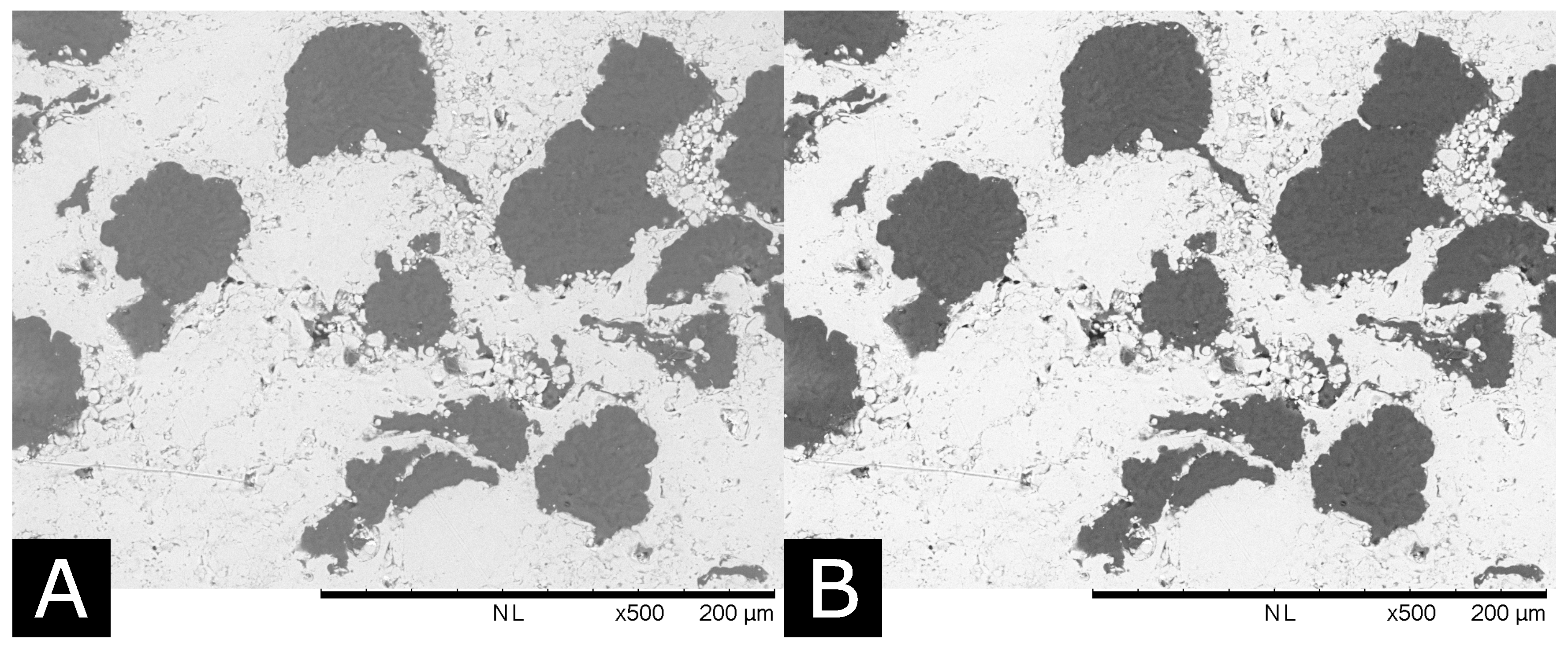
In addition to this, two further sets of images were taken for three of the samples tested. For these images the brightness and contrast of the images were varied. The samples were not moved between images and the magnification used was constant. Examples of the extremes of each set are shown in Figure 1A,B for brightness and Figure 2A,B for contrast, these images will be used to evaluate the repeatability of the image segmentation procedure compared to other methods.
2.3. Proposed Image Segmentation Procedure
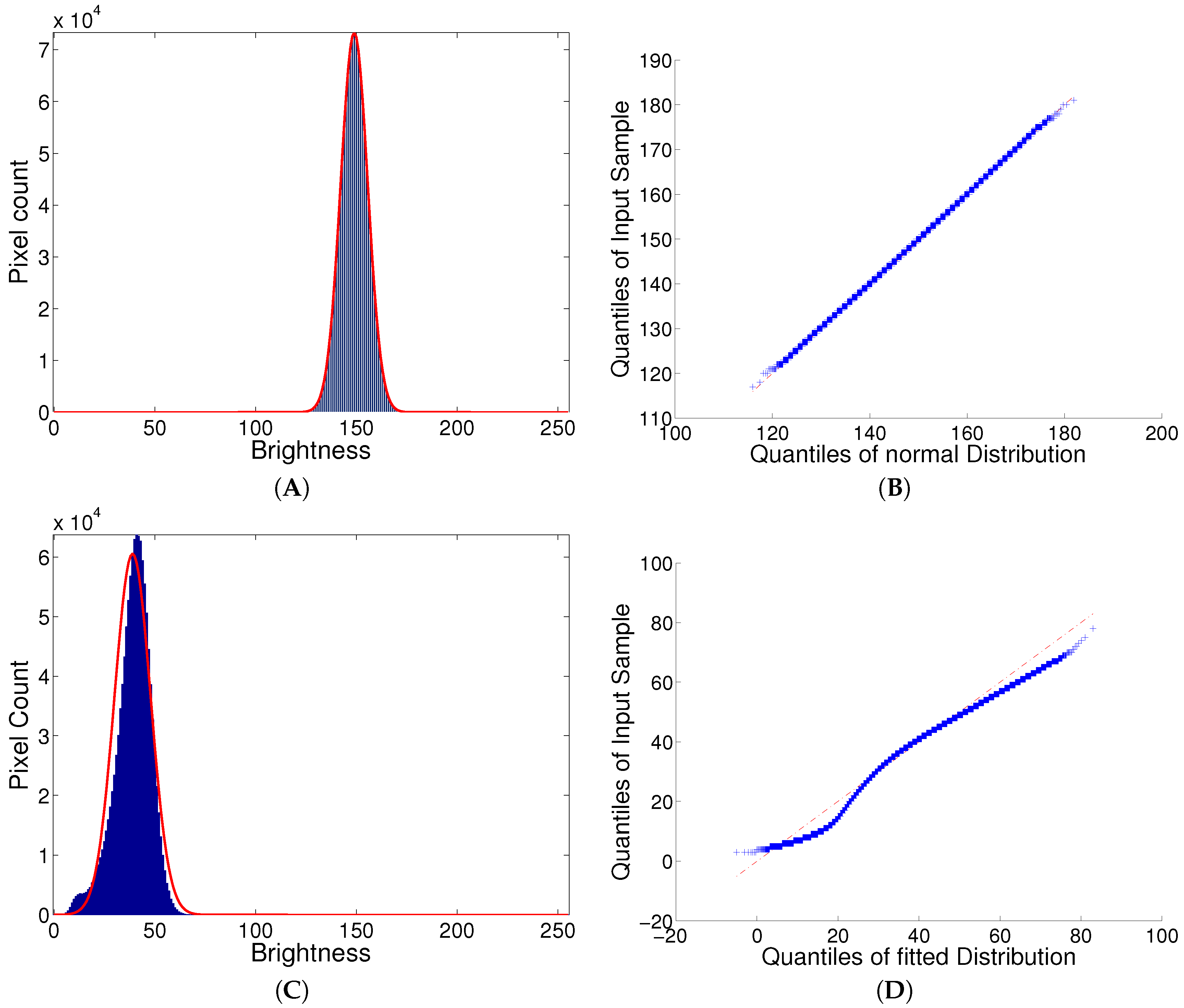
Each phase in the micrograph should be represented by normally distributed brightness values in the final image. This assumption has been verified by acquiring images with the settings as described above but with a magnification of 10,000×. These images were taken so a single phase was present in the frame. A histogram of one of these images with a normal distribution fitted to it is shown in Figure 3A while Figure 3B shows a quartile-quartile plot of the data and the fitted normal distribution.
Compliance to normal distributions is observed for metal phases in both 601 and 320, and polyester in 601. hBN in 320 has not been shown to follow a normal distribution as the tail on the dark side is too large as shown in Figure 3C,D. Matějíček et al. [14] showed that the hBN phase in these coatings contains some porosity, it is thus assumed that the hBN in these areas is normally distributed and the additional material in the darker tail is porosity. This assumption allows a general procedure to be developed, as described below. This assumption should be verified for any new material the process is used for.
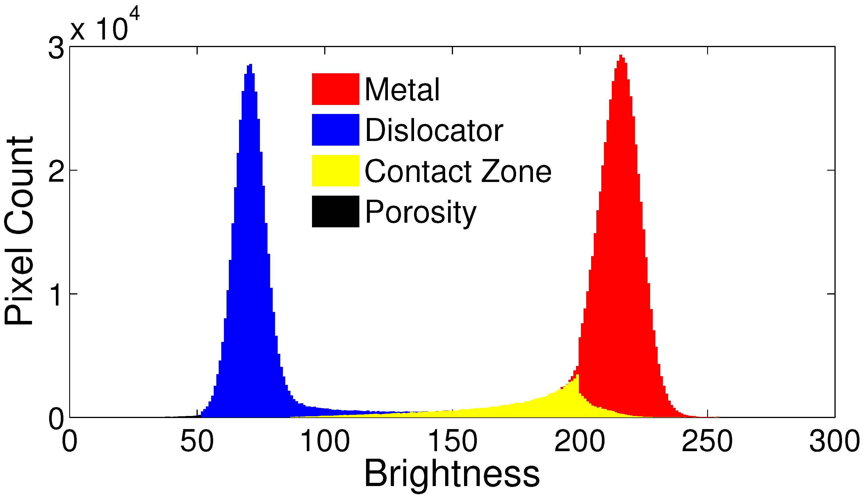
Figure 4 shows a histogram from a full image of an example microstructure (601-55). As shown the histogram consists of two peaks which approximate normal distributions. Between the peaks the level is higher than would be expected if the histogram were simply a combination of normal distributions. As each phase should be represented by a normal distribution optimum threshold points can be found by fitting normal distributions to each of these peaks.
The equation describing a normal distribution is given in Equation (1). In which S is a scale parameter. is the mean of the distribution and, as the distribution is symmetrical, the centre of the peak. is the standard deviation of the distribution. This curve is fitted to the histogram of the image by setting the above parameters.
The centre of each peak can be found by splitting the histogram at a point given by Otsu’s method and taking a weighted average of the top 11 points in each region (excluding any over exposed pixels). With this as the mean, the maximum value of the line is scaled to the the peak by setting the scale parameter S in Equation (1) to the maximum value from the histogram for that peak. The deviation parameter is set by minimising the least squares error between the line described by Equation (1) and the points from to again excluding overexposed pixels.
Figure 4 shows the histogram with scaled Gaussian curves for the dislocator and metal phase fitted as described above. The blue line in the figure shows the number of pixels not described by the fitted curves. As shown for the central section and the darkest area of the histogram this is more than 50% of the pixels at some brightness levels.
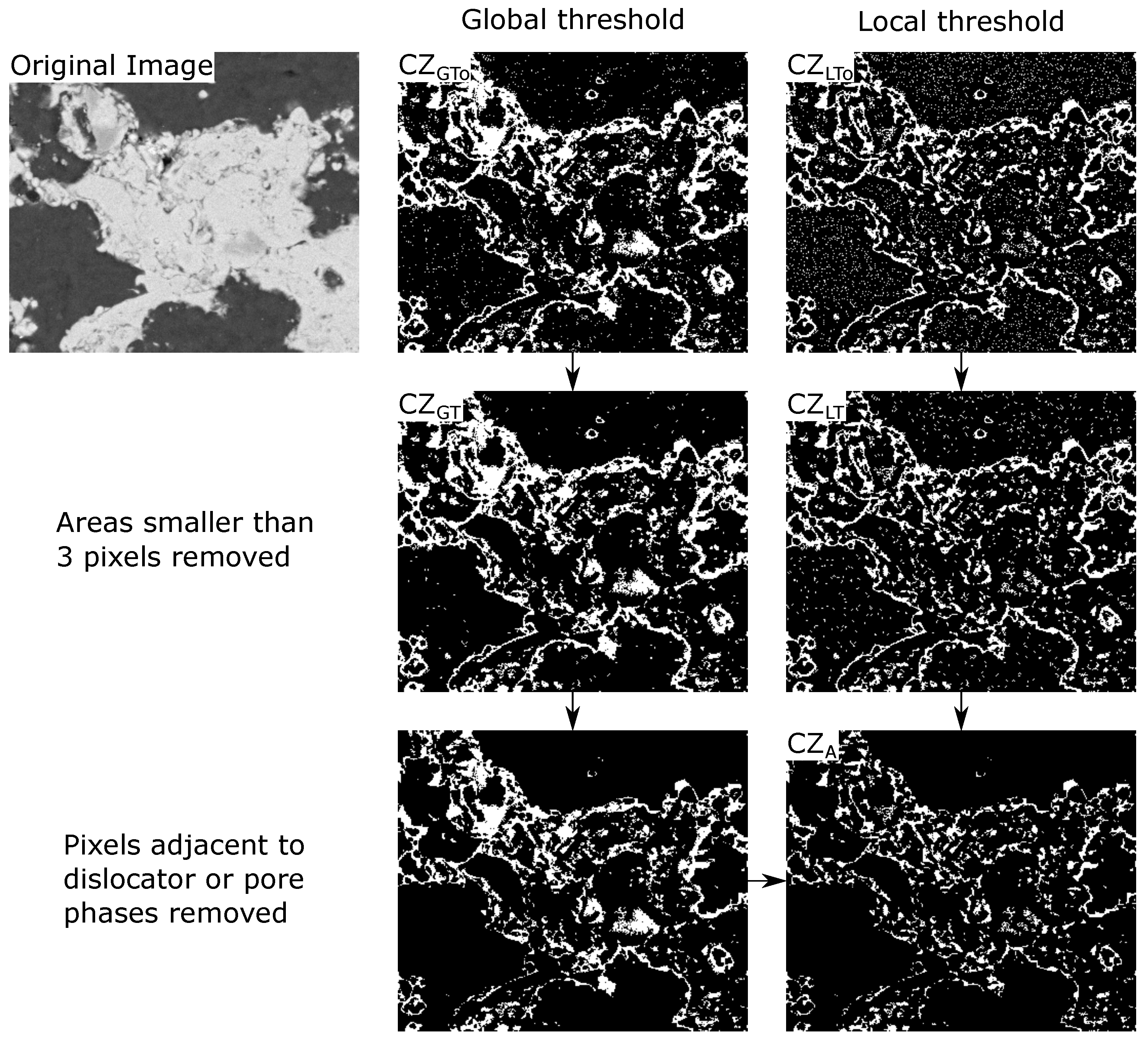
Pixels at brightness levels that are not well explained by either normal distribution (>) are considered as porosity if they are darker than the peak for the dislocator phase. If they are brighter than this they form the set of pixels: , an example of this set is shown in Figure 5. The resulting pixel set contains several features which are not cracks. Smudge type areas, transitions from the metal phase to the dislocator phase and some isolated pixels are included in this set. The following image processing steps remove these areas.
In order to remove smudge type areas a local threshold is used. A new image is created from the original with pixels belonging to the pore and dislocator phases replaced by random values from the distribution that describes the metal phase. The deviation from the local (15 by 15 pixels) mean is calculated for each pixel in this image. Pixels which deviate from the local mean by or less form the set of pixels: , an example of this set is shown in Figure 5. This includes some random pixels from the dislocator and pore phases but these are removed in a later step.
Isolated areas smaller than three pixels are then removed from the pixel sets and resulting in two new pixel sets: and respectively.
To remove pixels surrounding the dislocator and pore phases, these phases are dilated by a single pixel in each direction and the result removed from . This results in none of the cracks extending to the dislocator phase. The contact zone or cracks phase () is then found as the intersection between the sets: . This process is summarised in Figure 5.
To reconnect the contact zone phase with the dislocator and pore phases, the union of the pore, dislocator and cracks phases is dilated by a single pixel in each direction and thinned to a minimally connected stroke. These pixels are added to the cracks phase if they were originally members of either or . Pixels originally belonging to the dislocator phase are then removed from this set. This is described by Equation (2).
Pixels are then added to to force 4-connectivity (shared pixel edge) in previously 8-connected (shared pixel corner) bodies, while this step is technically un-physical it is necessary to produce physical behaviour for diagonal cracks. Lastly, is skeletalised and pixels which were originally part of the dislocator or pore phase are removed resulting in the contact zone phase (). Pixels removed from the crack phase are allocated to the metal phase if they are brighter than the threshold determined by Otsu’s method, otherwise they are allocated to the dislocator phase. The process of reconnecting the cracks to other phases and the subsequent processing is summarised in Figure 6.
2.4. Model Formulation
The processed phase maps were converted to a finite element mesh by the direct pixel to element method, giving one element per pixel with nodes at the corners. Boundary conditions of and C are applied to the top and bottom boundaries respectively, thus giving a temperature gradient through the material, the sides of the material are considered insulated. The static thermal problem was then solved by a purpose written matlab program. Using a uniform square mesh with purpose written code provides substantial improvements over commercial codes, not least as the model does not have to be exported after image segmentation. The finite element code is provided in the additional material of this work. Typical time for image processing, mesh generation and solution was around 2 min for a 900 by 900 pixel area.
2.4.1. Material Models
The material models used for each phase of the microstructure are summarised in Table 2. These are taken from values measured from large scale samples and are used without modification. Pixels belonging to the crack phase are assumed to be metallic with a crack much smaller than the pixel size. Thus the density and specific heat of the crack phase set the same as the metal phase. The effect of varying the conductivity of this phase will be investigated.
2.4.2. Other Threshold Methods
The image to model process has been repeated using the Otsu [12] and Bolot [9] methods for image segmentation. As the materials used consist of three phases and the alternative methods are for use with two phase materials for the comparative sections of this work the novel method will be used to segment into a phase of metal and a single phase of cracks, porosity and dislocator which is given the properties of porosity. Alternative methods will also split the image into two phases which will be assigned the properties for the metal matrix and the porosity as given in Table 2.
2.5. RVE Estimation
The method of RVE estimation described by Kanit et al. [22] will be used. This is simply the modelled areas and number of models which produces a standard error for the properties of interest of less than 5%. Although other methods exist these are less conservative. Hence, This approach was chosen because it provided the most robust assessment of the segmentation method proposed.
2.6. Experimental Methods
The density of the samples has been measured by the water displacement method using an Archimedes balance apparatus. Five measurements were taken from separate samples ( mm) for each material.
For each material investigated three diffusivity measurements were taken from separate samples. Measurements were taken at 40 C as this is the closest to room temperature possible. Measurements were taken on a flashline 3000 laser flash diffusivity apparatus (Anter Corporation, Pittsburgh, PA, USA). This has been calibrated to output both diffusivity and heat capacity of the sample with confidence bounds at . Combined with the density measurements this allows the thermal conductivity to be calculated.
3. Results
3.1. RVE Validation
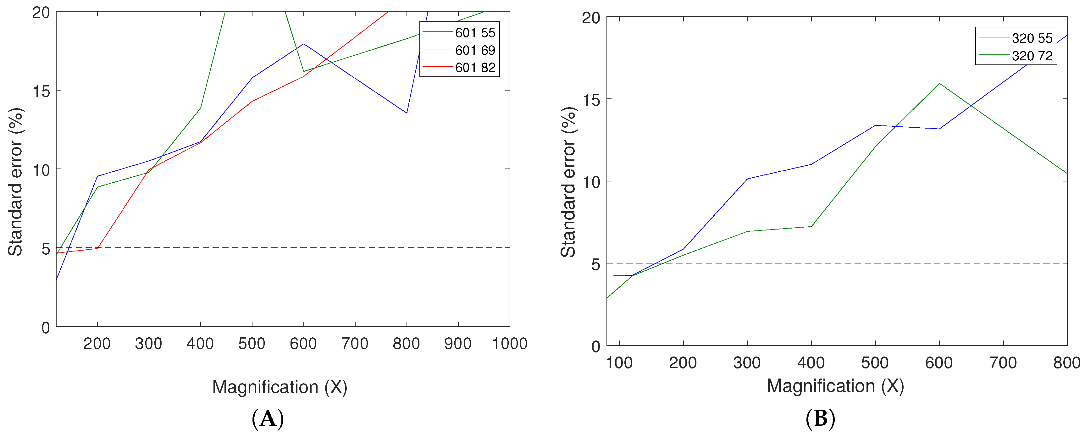
The Results from the RVE estimation are shown in Figure 9A,B for 601 and 320 respectively. As shown the standard error is below the 5% error threshold for 15 images taken at 120× for both 601 and 320. This means that a set of fifteen images is adequate to estimate the bulk properties with 5% random error at the given magnification. As such, where property estimates are made in this work, they will be the average from 15 models at a magnification of 120×.
3.2. Comparison to Experiment
3.2.1. Specific Heat and Density
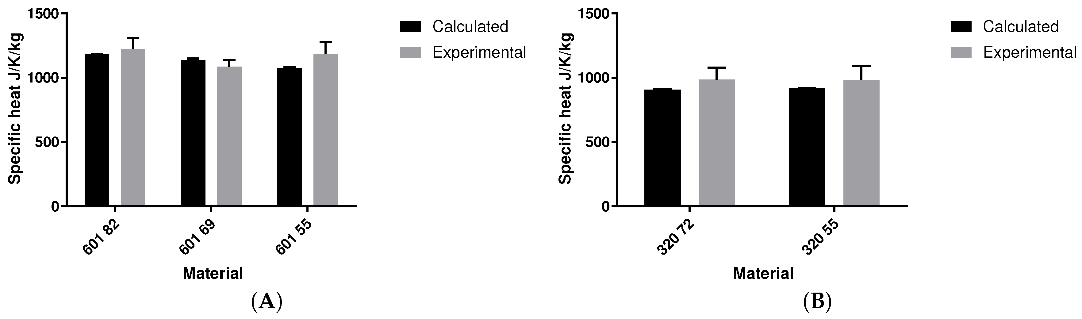
The modelled specific heat and density are outputs of the image segmentation procedure as they are simply the average of the phase properties weighted by their composition. These results are shown in Table 3 for each coating and each hardness. Modelled densities are shown in the context of the experimental results in Figure 10. The calculated specific heats are shown in Figure 11.
As shown the image segmentation procedure is able to produce estimates for the density and specific heats of the samples to within experimental error for 601. For 320 the density is over estimated, this may be due to difficulty in separating porosity from hBN or due to retained binder (latex) around the hBN.
3.2.2. Thermal Conductivity Results
As only a single reference provides an estimate for the conductivity of the contact zone phase the effect of varying its conductivity is investigated here. Figure 12A,B show the change in overall conductivity with changes in conductivity of the contact zone. As seen by Zivelonghi et al. [13] insulating behaviour is seen below with little additional effect with lower conductivities.
As with Zivelonghi et al. [13] the closest match to the measured values is found for however as an underestimate is expected for the 2D case this value should not be used. Since the exact value is unknown, the essentially insulating case of will be used for future modelling. This is compared to the experimental value in Figure 13 below.
For the AlSi polyester the model under predicts the thermal properties as expected. This under prediction is larger as a percentage of the actual value for softer batches with poor connectivity of the metal phase. For the AlSi hBN abradable a large over prediction is seen. Matějíček et al. and others have noted that residual binder surrounds the hBN particles [14,23,24]. This isolates the hBN from the heat flow in the metal matrix. If the conductivity of the hBN phase is reduced to that of the binder used the calculated conductivity gives the expected under prediction as shown in Figure 13B labelled no hBN.
3.3. Comparison to Alternative Techniques
For this section of the work, the image segmentation technique is used in a two phase mode. The contact zone, dislocator and porosity are grouped into a single phase which is given the properties of porosity. Results in this section should only be used to compare between techniques, not to provide absolute estimates.
Figure 14 shows the mean conductivity results from the ‘brightness’ set of images (described in Section 2.2 paragragh 2) for each threshold method tested. As these are binary models of three phase materials comparison to experimental data is not relevant. For each material the Otsu method gives the highest prediction indicating as others have concluded that this method is unable to identify cracks leading to over predictions of material properties [11].
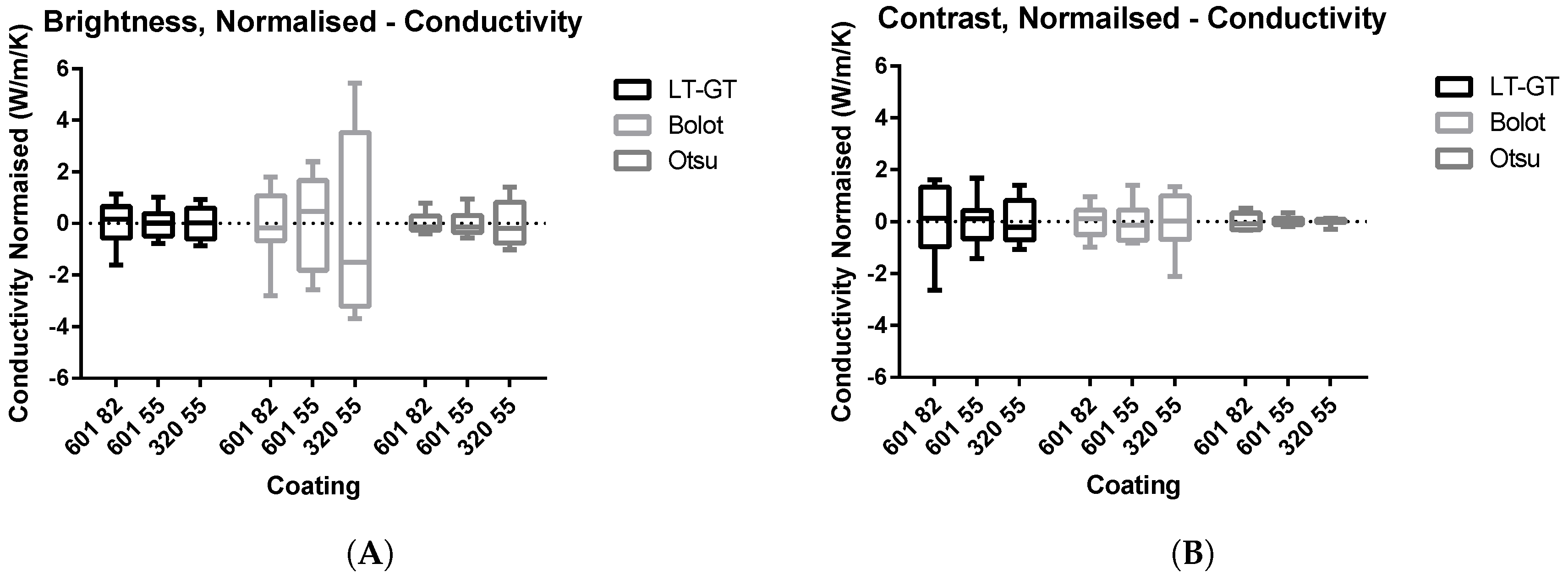
The repeatability of each method has also been investigated. Figure 15 shows box plots of the conductivity results for each threshold method and each coating tested. These results have been normalised by subtracting the mean result of each set. Figure 15A shows that the proposed segmentation technique is repeatable despite changes in brightness of the input image. The proposed method out performs the relevant alternative method proposed by Bolot et al. [3] in this respect. Adequate repeatability is found with changes in contrast (Figure 15B) although the range of results is slightly larger than those generated by the Bolot method. Although the range of results generated by the Otsu method is smaller in both cases, this method is inappropriate for property estimation due to over predictions discussed above.
The systematic error produced with changes in brightness or contrast can be investigated by linear regression of the results. Table 4 summarises these results, ideally there would be no significant trend in the results with respect to changes in brightness or contrast of the input image. As shown the suggested method has no significant bias in five out of six of the conditions tested, in this respect it outperforms both the Otsu and Bolot methods of image segmentation. However it should be noted that changes in the result from the Otsu method are small and not of practicable importance.
4. Discussion
An automatic method for image segmentation has been developed which is capable of automatically extracting a phase of cracks from the microstructure as described by Zivelonghi et al. [13]. The method has been compared to other current methods and is shown to be as or more repeatable than alternatives [3] which threshold in the same region with changes in brightness or contrast of the input image. In addition the method has physical underpinnings which justify the selection of threshold points for this application.
This segmentation method produced estimates of density and specific heat that were within experimental error of measured values. This extends the work on porosity of Deshpande et al. [8] and Matějíček et al. [14] to other properties which are simply a volumetric mean of the components of the composite.
Under predictions were seen for modelled thermal conductivity results as is to be expected of two dimensional models due to the loss of connectivity in the third dimension. As with Zivelonghi et al. [13] the overall conductivity was strongly dependent on the contact zone or crack conductivity. The proper value to be used for this variable remains unknown.
Separately these results also explain some phenomena seen in high speed wear testing of these materials. Variation in wear behaviour is seen across the width of the rub track of the same scale as variation between the spray batches shown here [24]. Models made from m images showed standard deviation in thermal conductivity results of between 46% and 66% of the mean value (Figure 9). Thus roughly 30% of such areas will have properties equal to the bulk properties of one of the adjacent batches (50% change in value, one standard deviation). This rate decreases as the sampled area increases, 2% of mm sections are expected to vary from the bulk mean by 50% or more. As such local variation in the abradables is in the same scale as variation between batches and can be expected to produce the same changes in wear mechanism.
5. Conclusions
An automatic image segmentation method has been developed which allows automatic separation of a phase of cracks from a microstructure image. Estimates of the density and the specific heat capacity of the material could be made to within experimental error and expected under predictions for thermal conductivity were observed.
The segmentation method was shown to have less systematic bias with brightness and contrast than other available methods. Random error was also lower than seen for competing methods for changes in brightness of input image and was similar to competing methods for changes in contrast of the input image.
Supplementary Materials
The following are available online at https://www.mdpi.com/2079-6412/7/10/166/s1, LtGt: the image segmentation code, small_FE: the finite element code. The image segmentation code and the finite element code for static heat transfer are avalible online in the matlab file exchange.
Author Contributions
Michael Watson conceived the segmentation method and the methods to test it, implemented the method, carried out the experiments analysed the data and wrote the paper with additional guidance and help in method development form Matthew Marshall.
Conflicts of Interest
The authors declare no conflict of interest.
References
- Faraoun, H.; Seichepine, J.; Coddet, C.; Aourag, H.; Zwick, J.; Hopkins, N.; Sporer, D.; Hertter, M. Modelling route for abradable coatings. Surf. Coat. Technol. 2006, 200, 6578–6582. [Google Scholar] [CrossRef]
- Bolot, R.; Seichepine, J.; Vucko, F.; Coddet, C.; Sporer, D.; Fiala, P.; Bartlett, B. Thermal Conductivity of AlSi/Polyester Abradable Coatings. In Proceedings of the Thermal Spray 2008: Crossing Borders (DVS-ASM), Maastricht, The Netherlands, 2–4 June 2008; pp. 1056–1061. [Google Scholar]
- Bolot, R.; Seichepine, J.; Qiao, J.; Coddet, C. Predicting the thermal conductivity of AlSi/polyester abradable coatings: effects of the numerical method. J. Therm. Spray 2011, 20, 39–47. [Google Scholar] [CrossRef]
- Fizi, Y.; Yamina, M.; Lahmar, H. Modeling of the Mechanical Behaviour of Abradable Coatings for the Aeronautical Industry. In Proceedings of the 2nd International Conference on Aeronautics Sciences, ICAS 2015, Oran, Algeria, 3–4 November 2015. [Google Scholar]
- Bolelli, G.; Candeli, A.; Koivuluoto, H.; Lusvarghi, L.; Manfredini, T.; Vuoristo, P. Microstructure-based thermo-mechanical modelling of thermal spray coatings. Mater. Des. 2015, 73, 20–34. [Google Scholar] [CrossRef] [Green Version]
- Gupta, M. Establishment of Relationships between Coating Microstructure and Thermal Conductivity in Thermal Barrier Coatings by Finite Element Modelling. Master’s Thesis, University West, Gothenburg, Sweden, 2010. [Google Scholar]
- Qiao, J.H.; Bolot, R.; Liao, H.L.; Bertrand, P.; Coddet, C. A 3D finite-difference model for the effective thermal conductivity of thermal barrier coatings produced by plasma spraying. Int. J. Therm. Sci. 2013, 65, 120–126. [Google Scholar] [CrossRef]
- Deshpande, S.; Kulkarni, A.; Sampath, S.; Herman, H. Application of image analysis for characterization of porosity in thermal spray coatings and correlation with small angle neutron scattering. Surf. Coat. Technol. 2004, 187, 6–16. [Google Scholar] [CrossRef]
- Bolot, R.; Qiao, J.H.; Bertrand, G.; Bertrand, P.; Coddet, C. Effect of thermal treatment on the effective thermal conductivity of YPSZ coatings. Surf. Coat. Technol. 2010, 205, 1034–1038. [Google Scholar] [CrossRef]
- Coffman, V.R.; Reid, A.C.E.; Langer, S.A.; Dogan, G. OOF3D: An image-based finite element solver for materials science. Math. Comput. Simul. 2012, 82, 2951–2961. [Google Scholar] [CrossRef]
- Qiao, J.H.; Bolot, R.; Liao, H. Finite element modeling of the elastic modulus of thermal barrier coatings. Surf. Coat. Technol. 2013, 220, 170–173. [Google Scholar] [CrossRef]
- Otsu, N. A threshold selection method from gray-level histograms. Automatica 1975, 9, 62–66. [Google Scholar] [CrossRef]
- Zivelonghi, A.; Cernuschi, F.; Peyrega, C.; Jeulin, D.; Lindig, S.; You, J. Influence of the dual-scale random morphology on the heat conduction of plasma-sprayed tungsten via image-based FEM. Comput. Mater. Sci. 2013, 68, 5–17. [Google Scholar] [CrossRef]
- Matějíček, J.; Kolman, B.; Dubský, J.; Neufuss, K.; Hopkins, N.; Zwick, J. Alternative methods for determination of composition and porosity in abradable materials. Mater. Charact. 2006, 57, 17–29. [Google Scholar] [CrossRef]
- Wiederkehr, T.; Klusemann, B.; Gies, D.; Müller, H.; Svendsen, B. An image morphing method for 3D reconstruction and FE-analysis of pore networks in thermal spray coatings. Comput. Mater. Sci. 2010, 47, 881–889. [Google Scholar] [CrossRef]
- Dorvaux, J.; Lavigne, O.; Mevrel, R. Modelling the Thermal Conductivity of Thermal Barrier Coatings; NASA: Washington, DC, USA, 1998.
- Leo, M.; Looney, D.; Orazio, T.D.; Mandic, D.P.; Member, S. Identification of Defective Areas in Composite Materials by Bivariate EMD Analysis of Ultrasound. IEEE Trans. Instrum. Measur. 2012, 61, 221–232. [Google Scholar] [CrossRef]
- Chen, S.-H.; Perng, D.-B. Automatic optical inspection system for IC molding surface. J. Intell. Manuf. 2016, 27, 915–926. [Google Scholar] [CrossRef]
- Material Properties for hBN. Available online: http://www.matweb.com/search/datasheet.aspx?matguid=8fbbb7d47809493e9afbb7778657d5bb&ckck=1 (accessed on 21 November 2016).
- Material Properties for Polyester. Available online: http://www.professionalplastics.com/professionalplastics/ThermalPropertiesofPlasticMaterials.pdf (accessed on 15 October 2016).
- Material Properties for Air. Available online: http://www.engineeringtoolbox.com/air-properties-d_156.html (accessed on 10 October 2016).
- Kanit, T.; Forest, S.; Galliet, I.; Mounoury, V.; Jeulin, D. Determination of the size of the representative volume element for random composites: Statistical and numerical approach. Int. J. Solids Struct. 2003, 40, 3647–3679. [Google Scholar] [CrossRef]
- Johnston, R.; Evans, W. Freestanding abradable coating manufacture and tensile test development. Surf. Coat. Technol. 2007, 202, 725–729. [Google Scholar] [CrossRef]
- Fois, N.; Watson, M.; Marshall, M. The influence of material properties on the wear of abradable materials. Proc. Inst. Mech. Eng. Part J J. Eng. Tribol. 2016, 231, 240–253. [Google Scholar] [CrossRef]
Figure 1.
(A) The brightest and (B) darkest images from an example set used to evaluate the image segmentation algorithms.
Figure 1.
(A) The brightest and (B) darkest images from an example set used to evaluate the image segmentation algorithms.
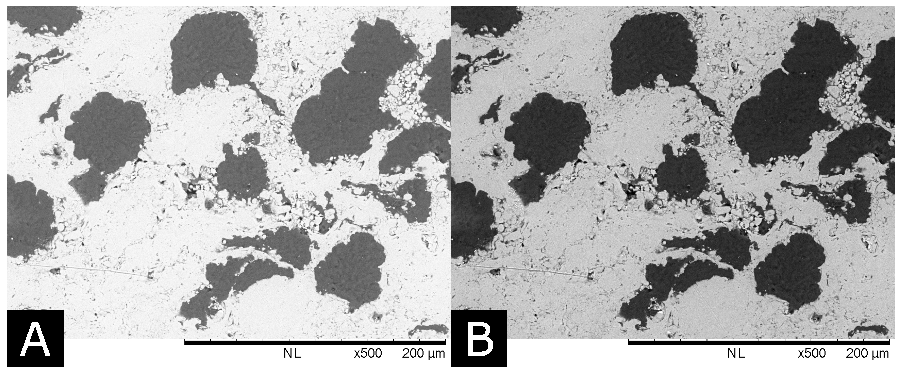
Figure 2.
(A) The lowest and (B) highest contrast images from an example set used to evaluate the image segmentation algorithms.
Figure 2.
(A) The lowest and (B) highest contrast images from an example set used to evaluate the image segmentation algorithms.

Figure 3.
(A) A histogram of an image containing only metal phase (601); (B) quartile-quartile plot of the data in A vs. the fitted distribution; (C) a histogram of an image containing only hBN phase (320); (D) quartile-quartile plot of the data in C vs. the fitted distribution.
Figure 3.
(A) A histogram of an image containing only metal phase (601); (B) quartile-quartile plot of the data in A vs. the fitted distribution; (C) a histogram of an image containing only hBN phase (320); (D) quartile-quartile plot of the data in C vs. the fitted distribution.

Figure 4.
A histogram of an image of the 601-55 microstructure with normal distributions fitted to both peaks.
Figure 4.
A histogram of an image of the 601-55 microstructure with normal distributions fitted to both peaks.
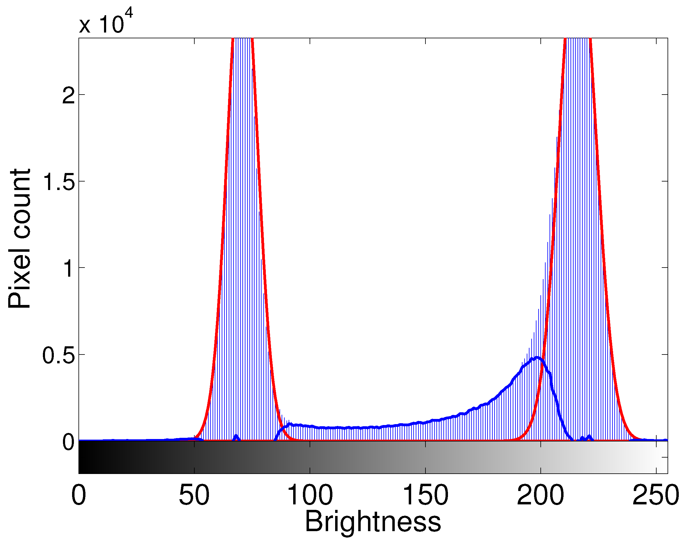
Figure 5.
The threshold methods used and their combination to generate the pixel set , the example shown is from an image of a 601-82 microstructure.
Figure 5.
The threshold methods used and their combination to generate the pixel set , the example shown is from an image of a 601-82 microstructure.

Figure 6.
The process of reconnecting the cracks to other phases and subsequent image processing, the example shown is from an image of a 601-82 microstructure.
Figure 6.
The process of reconnecting the cracks to other phases and subsequent image processing, the example shown is from an image of a 601-82 microstructure.
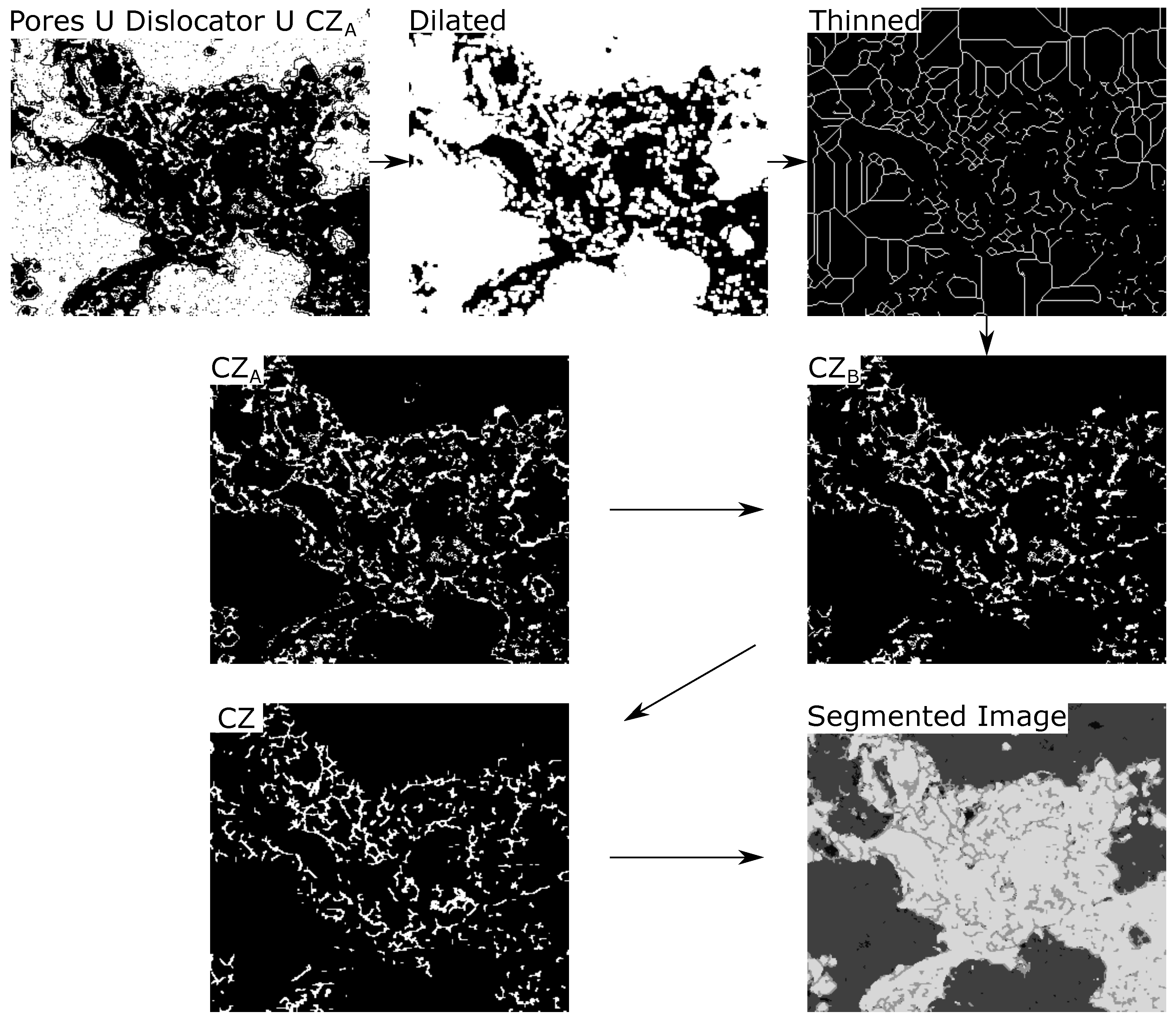
Figure 7.
A histogram of the brightness of pixels in each phase as segmented by the image analysis described above, the original image is of a 601-55 microstructure.
Figure 7.
A histogram of the brightness of pixels in each phase as segmented by the image analysis described above, the original image is of a 601-55 microstructure.

Figure 8.
Side by side comparison of an original microscope image of a 601-82 microstructure and the result of the image segmentation procedure.
Figure 8.
Side by side comparison of an original microscope image of a 601-82 microstructure and the result of the image segmentation procedure.
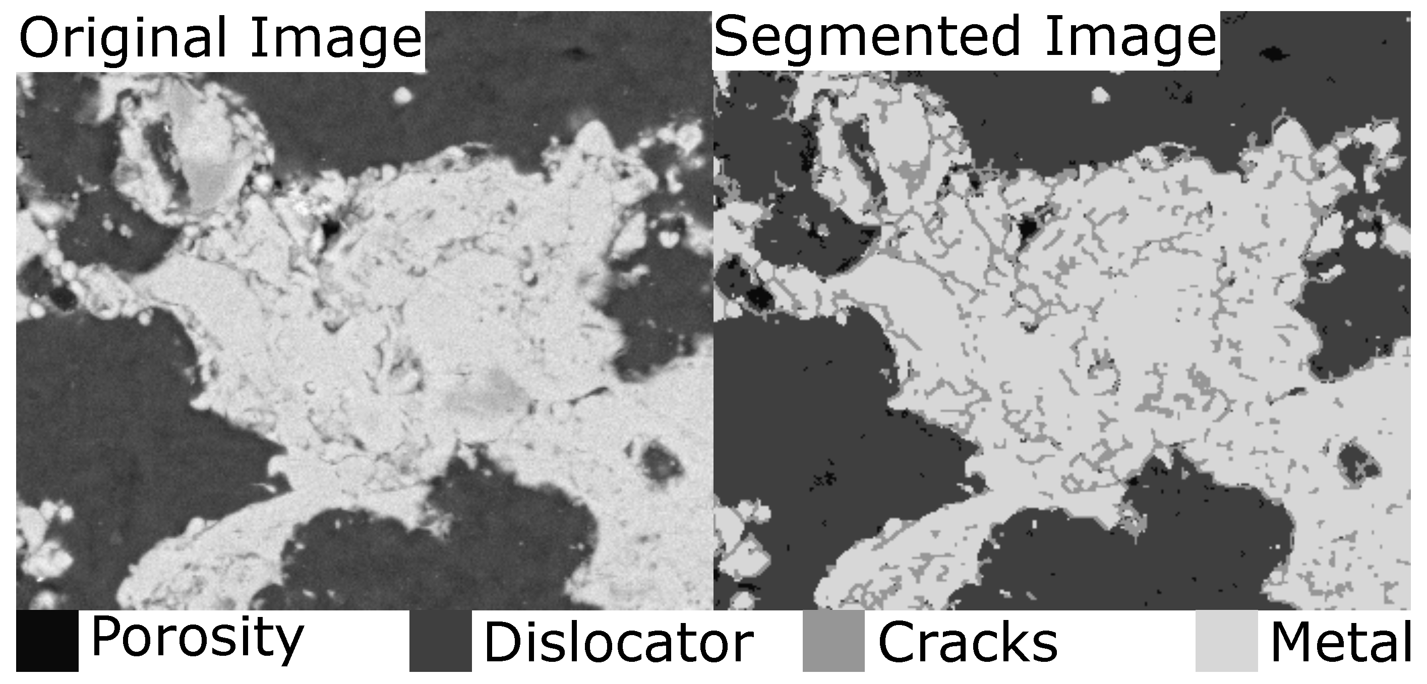
Figure 9.
Standard error vs magnification of input image for the conductivity results from (A) 601 (AlSi-polyester) and (B) 320 (AlSi-hBN) respectively.
Figure 9.
Standard error vs magnification of input image for the conductivity results from (A) 601 (AlSi-polyester) and (B) 320 (AlSi-hBN) respectively.

Figure 10.
Calculated vs. measured density for (A) 601 (AlSi-polyester) and (B) 320 (AlSi-hBN) respectively.
Figure 10.
Calculated vs. measured density for (A) 601 (AlSi-polyester) and (B) 320 (AlSi-hBN) respectively.
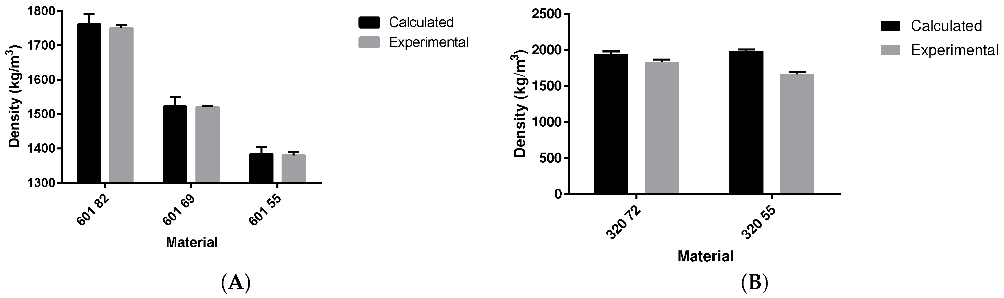
Figure 11.
Calculated vs. measured specific heat capacity for (A) 601 (AlSi-polyester) and (B) 320 (AlSi-hBN) respectively.
Figure 11.
Calculated vs. measured specific heat capacity for (A) 601 (AlSi-polyester) and (B) 320 (AlSi-hBN) respectively.

Figure 12.
The overall conductivity when the conductivity of the contact zone phase is changed up to that of the metal phase in (A) 601 and (B) 320. Error bars represent standard error.
Figure 12.
The overall conductivity when the conductivity of the contact zone phase is changed up to that of the metal phase in (A) 601 and (B) 320. Error bars represent standard error.
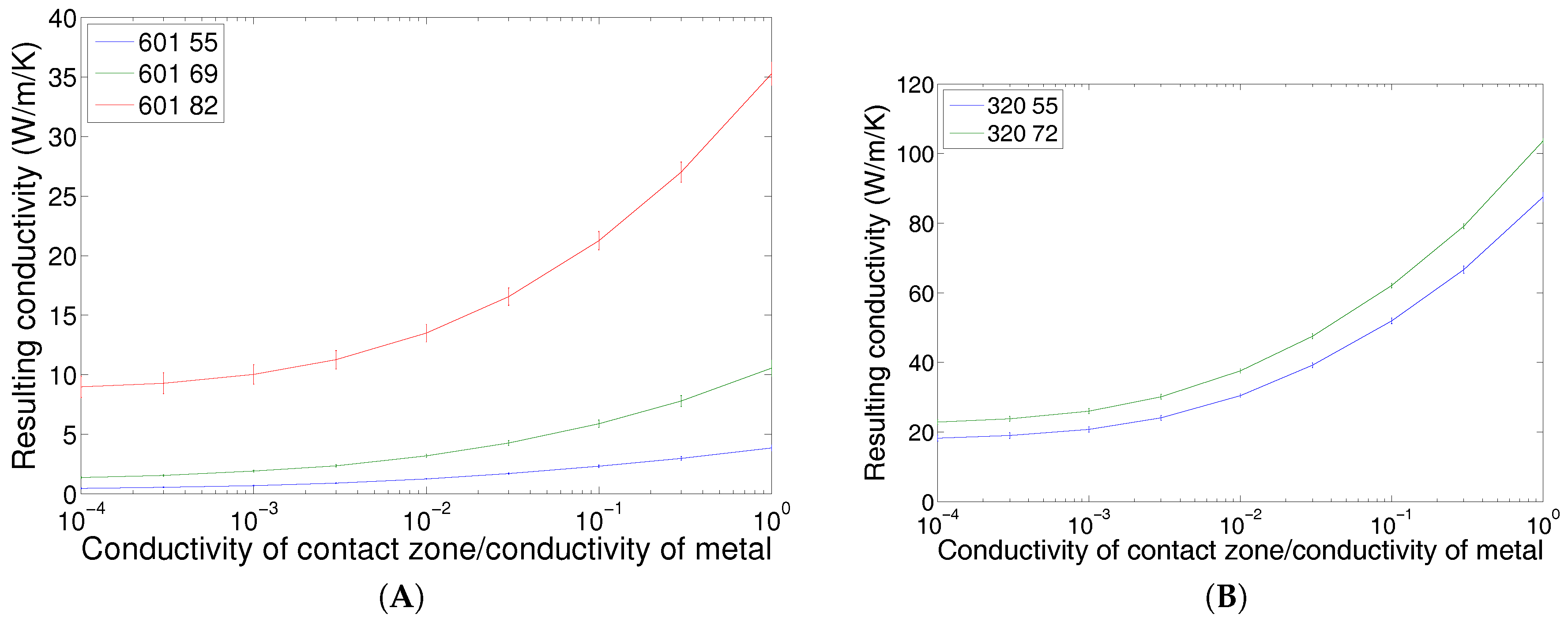
Figure 13.
Calculated and experimental values for the thermal conductivity of the (A) AlSi polyester and (B) AlSi hBN abradables. Error bars represent standard error.
Figure 13.
Calculated and experimental values for the thermal conductivity of the (A) AlSi polyester and (B) AlSi hBN abradables. Error bars represent standard error.
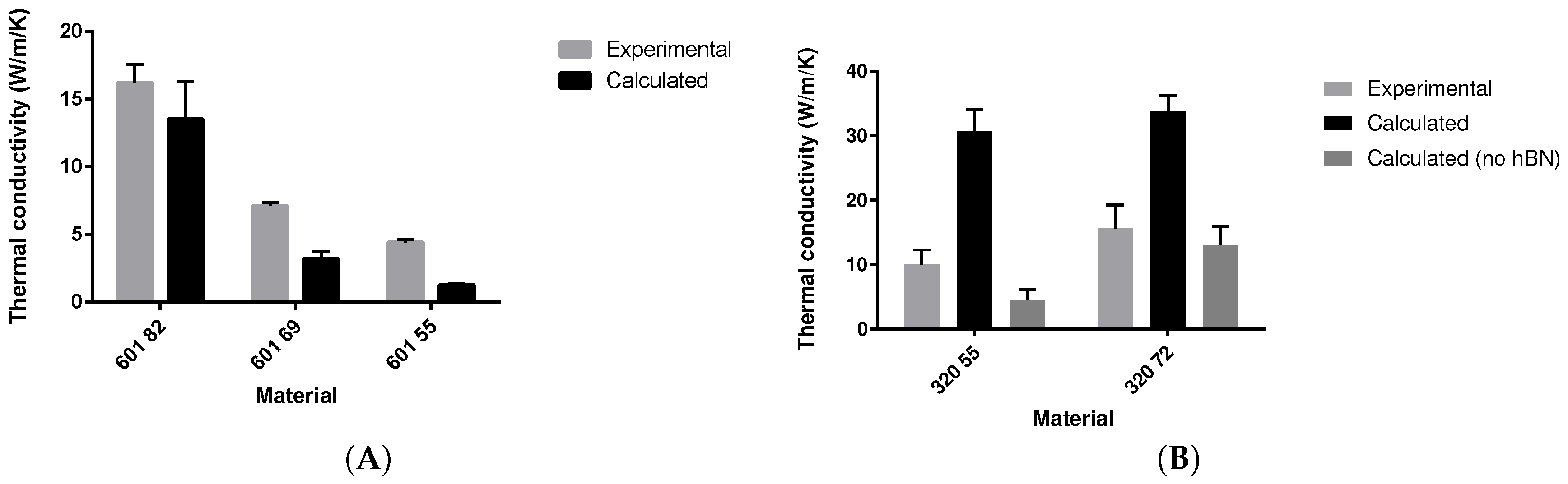
Figure 14.
The mean calculated conductivity results for each of the threshold methods tested over the brightness set of images.
Figure 14.
The mean calculated conductivity results for each of the threshold methods tested over the brightness set of images.
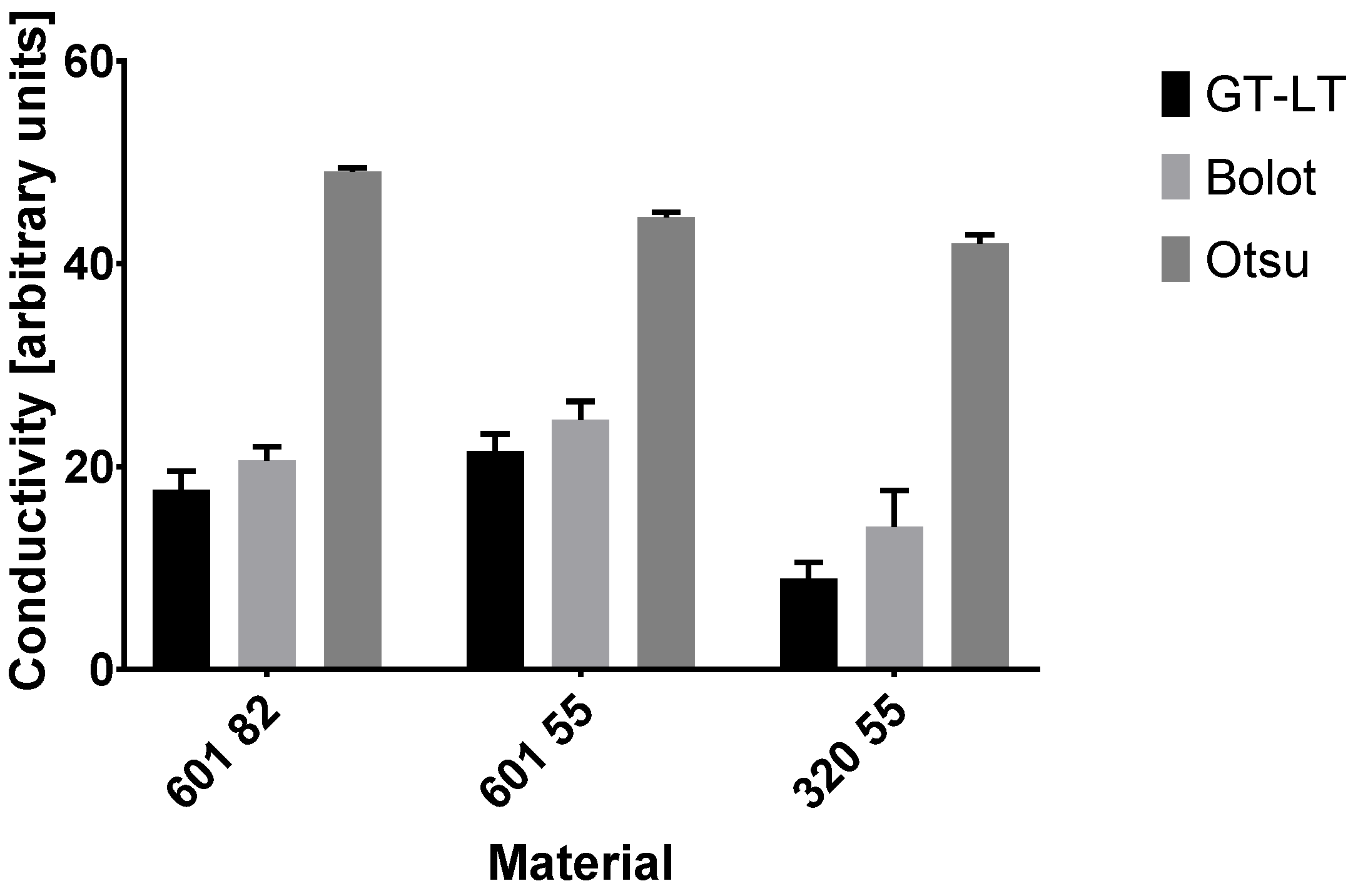
Figure 15.
The variation of conductivity results from different threshold methods with changes in (A) brightness and (B) contrast.
Figure 15.
The variation of conductivity results from different threshold methods with changes in (A) brightness and (B) contrast.

Table 1.
Magnifications of images taken and the corresponding edge length of the 900 by 900 pixel square used for modelling.
Table 1.
Magnifications of images taken and the corresponding edge length of the 900 by 900 pixel square used for modelling.
| Magnification (×) | Model Size (m) |
|---|---|
| 80 | 1223 |
| 120 | 815 |
| 200 | 489 |
| 300 | 326 |
| 400 | 245 |
| 500 | 196 |
| 600 | 163 |
| 800 | 122 |
Table 2.
Material properties used in the finite element models.
| Material | Conductivity W/m/K | Specific Heat Capacity Cp J/kg/K | Density kg/m | Reference |
|---|---|---|---|---|
| AlSi(12%) | 130 | 910 | 2700 | [9] |
| hBN | 33 | 808 | 2100 | [19] |
| Polyester | 0.15 | 1350 | 900 | [20] |
| Pores | 0.0257 | 1005 | 1.205 | [21] |
| Cracks | - | 910 | 2700 | [9] * |
| Dimensionality | - |
* Specific heat capacity and density of the metal phase is used for the crack phase as discussed in main text.
Table 3.
Calculated composition and material properties of the coatings based on image analysis of 15 micrographs from each image at 120X magnification with standard error ().
Table 3.
Calculated composition and material properties of the coatings based on image analysis of 15 micrographs from each image at 120X magnification with standard error ().
| Coating-HR15Y | Metal (%) | CZ (%) | Dislocator (%) | Porosity (%) | Density (kg/m) | (J/K/kg) |
|---|---|---|---|---|---|---|
| 601-82 | ||||||
| 601-69 | ||||||
| 601-55 | ||||||
| 320-72 | ||||||
| 320-55 |
Table 4.
Significance of non zero slope from linear regression of conductivity results from different threshold methods with changes in brightness and contrast.
Table 4.
Significance of non zero slope from linear regression of conductivity results from different threshold methods with changes in brightness and contrast.
| Coating | Variable | LT-GT | Bolot | Otsu |
|---|---|---|---|---|
| 601 55 | Brightness | NS | **** | * |
| 601 82 | Brightness | NS | * | *** |
| 320 55 | Brightness | NS | * | *** |
| 601 55 | Contrast | NS | ** | NS |
| 601 82 | Contrast | NS | *** | **** |
| 320 55 | Contrast | * | * | ** |
* NS stands for not significant and *, **, ***, **** indicate significance at the and levels respectively.
© 2017 by the authors. Licensee MDPI, Basel, Switzerland. This article is an open access article distributed under the terms and conditions of the Creative Commons Attribution (CC BY) license (http://creativecommons.org/licenses/by/4.0/).
Share and Cite
MDPI and ACS Style
Watson, M.; Marshall, M. A Novel Image Segmentation Approach for Microstructure Modelling. Coatings 2017, 7, 166. https://doi.org/10.3390/coatings7100166
AMA Style
Watson M, Marshall M. A Novel Image Segmentation Approach for Microstructure Modelling. Coatings. 2017; 7(10):166. https://doi.org/10.3390/coatings7100166
Chicago/Turabian StyleWatson, Michael, and Matthew Marshall. 2017. "A Novel Image Segmentation Approach for Microstructure Modelling" Coatings 7, no. 10: 166. https://doi.org/10.3390/coatings7100166
Note that from the first issue of 2016, this journal uses article numbers instead of page numbers. See further details here.