
Marching-on-in-Degree Time-Domain Integral Equation Solver for Transient Electromagnetic Analysis of Graphene


1
Department of Communication Engineering, Nanjing University of Posts and Telecommunications, Nanjing 210003, China
2
State Key Laboratory of Millimeter Waves, Southeast University, Nanjing 210096, China
3
Qualcomm Business Management (Shanghai) Co., Ltd., Shanghai 201203, China
4
Department of Information Engineering, Hefei University of Technology, Hefei 230009, China
*
Author to whom correspondence should be addressed.
Coatings 2017, 7(10), 170; https://doi.org/10.3390/coatings7100170
Submission received: 30 August 2017
/
Revised: 28 September 2017
/
Accepted: 13 October 2017
/
Published: 17 October 2017
(This article belongs to the Special Issue Modelling and Simulation of Coating)
Abstract
:The marching-on-in-degree (MOD) time-domain integral equation (TDIE) solver for the transient electromagnetic scattering of the graphene is presented in this paper. Graphene’s dispersive surface impedance is approximated using rational function expressions of complex conjugate pole-residue pairs with the vector fitting (VF) method. Enforcing the surface impedance boundary condition, TDIE is established and solved in the MOD scheme, where the temporal surface impedance is carefully convoluted with the current. Unconditionally stable transient solution in time domain can be ensured. Wide frequency band information is obtained after the Fourier transform of the time domain solution. Numerical results validate the proposed method.
1. Introduction
A single layer of graphite, i.e., the monolayer graphene sheet, has many ideal properties and considerable potential in terahertz communications [1], stealth technologies [2], solar cells [3], etc. The transfer matrix method (TMM) [2] and rigorous coupled wave analysis (RCWA) [4] are very efficient for some particular graphene structures. As for more general full-wave numerical simulation, various methods are available, including but not limited to the finite integration technique (FIT) [5], the finite element method (FEM) [6], the method of moments (MOM) [7,8], and the Nyström method [9,10]. For transient electromagnetic analysis, time domain techniques are preferred, e.g., the finite-difference time-domain (FDTD) [11,12,13], discontinuous Galerkin time domain (DGTD) method [14,15,16], and the time-domain integral equation (TDIE) method [17,18].
The TDIE method has been more and more popular in solving transient electromagnetic problems. The marching-on-in-degree (MOD) scheme [19,20,21,22,23,24,25] uses weighted Laguerre polynomials (WLPs) as the temporal basis functions, and involves no late-time instability, which may be encountered in the marching-on-in-time (MOT) scheme [26,27,28]. Generally, when handling resonant structures with a long tail current, many more degrees of WLPs are required. In this case, the frequency domain methods are recommended, but they may suffer from the ill-conditioned impedance matrix as well. When handling the potential internal resonance problems, the MOD scheme [19] and augmented electric field integral equation [22] might be the remedy.
In this paper, the MOD TDIE solver for the transient electromagnetic scattering of the graphene sheet is developed. The TDIE is based on the surface impedance boundary condition. The surface impedance is approximated by a vector fitting (VF) method, which has since its first introduction in 1999 widely applied for its robustness and efficiency [11,12,13,14,15,16,17,18,29,30,31,32,33,34]. Convolution of the temporal surface impedance and current is derived from properties of Laguerre polynomials.
2. Formulation
2.1. Modeling of Graphene and VF Method
The Kubo formula-based graphene sheet dispersive frequency domain intraband and interband conductivity are as follows:
where ω is the angular frequency, μc is the chemical potential, Γ is the phenomenological scattering rate (or relaxation time), T is the temperature, e is the electron charge, kB is the Boltzmann constant, and h is the Planck constant.
VF computes a rational approximation from the frequency domain data, using expressions in terms of complex conjugate pole-residue pairs. Graphene’s frequency domain surface impedance is as follows:
where al and cl are poles and residues, respectively. The real parts of al should be negative for causality and stability.
Calculating ρ(ω) at several frequencies with a set of starting poles presents the over-determined linear problem, which can be solved with the least squares method. It is repeated using new poles as starting poles in an iterative procedure until the convergence is achieved [29,30,31].
Graphene’s time domain surface impedance is [17]
denotes inverse Fourier transform, and u(t) is the unit step function.
2.2. TDIE and Temporal Convolution
Enforcing the surface impedance boundary condition, the TDIE is
|tan stands for tangential electric fields, S’ is the surface of graphene sheet illuminated by the transient electric field Einc(r,t), r and r’ are field and source point position vectors, , ∆tR = R/c, is the first derivative of current with respect to time t, * is the temporal convolution, and c, ε0, and μ0 are light velocity, permittivity and permeability in free space, respectively.
The j-th degree Laguerre polynomial is
The weighted Laguerre polynomial (WLP) is
s is the temporal scaling factor, and converges to zero. The highest degree of WLP is
t0 is the time delay of the signal, and B is the bandwidth of the incident pulse.
Given real (ai) < 0, we have [23]
NL is the highest degree of WLP, bl = al/s − 1/2, and al and cl are poles and residues in the VF method, respectively.
In the computer model, the infinitely thin graphene sheet is built as a plane (zero-thickness) with a triangle mesh. The induced current of graphene is expressed by both spatial and temporal basis functions as
NS is the number of inner edges of the triangles, Jn,j is the unknown coefficient, and fn(r) is the RWG basis function defined by the triangle mesh. Using WLPs as temporal basis functions eliminates the late-time oscillation.
With Equations (9) and (10),
where
Together with the property
we get
where
2.3. MOD Scheme
If the temporal derivative and integration terms [20] of the coefficients Jn,j and Equation (16) is substituted into Equation (5), we get
where
Following the Galerkin’s method with spatial testing functions fm(r), Equation (17) can be rewritten as
where
If a temporal testing procedure with is performed, we obtain the matrix equation of the i-th degree:
where
and
Rmn is the distance between centroids of the two triangles related to fm(r) and fn(r’).
The matrix equation is solved degree by degree (0 ≤ i ≤ NL), and the surface current can be obtained by Equations (10) and (28). After that, electromagnetic parameters, e.g., far field scattering, can be computed from the current.
3. Results and Discussion
Consider a 1 mm × 1 mm graphene sheet of μc = 0.01 eV and Γ = 5 × 10¹² s−1 at T = 300 K. Following Equations (1)–(4), poles al and residues cl of graphene’s surface impedance computed with VF when p = 2 are listed in Table 1. Negative real parts of al are required to ensure casualty and stability. Graphene’s surface impedances are computed and compared in Figure 1, where the results of VF are identical to those computed by the Kubo formula.
The graphene sheet is illuminated by the modulated Gaussian pulse
The central frequency f0 and frequency bandwidth fbw are 0.204 THz and 0.408 THz, respectively, and , is the unit vector of the incidence direction and along the –z direction in this example, tp = 3.5η, η = 6/(2πfbw).
The transient electromagnetic problem is solved using the MOD TDIE solver presented in Section 2. The graphene surface current is expressed by 313 RWGs and 80 WLPs. The scaling factor s is 9.0 × 10¹¹.
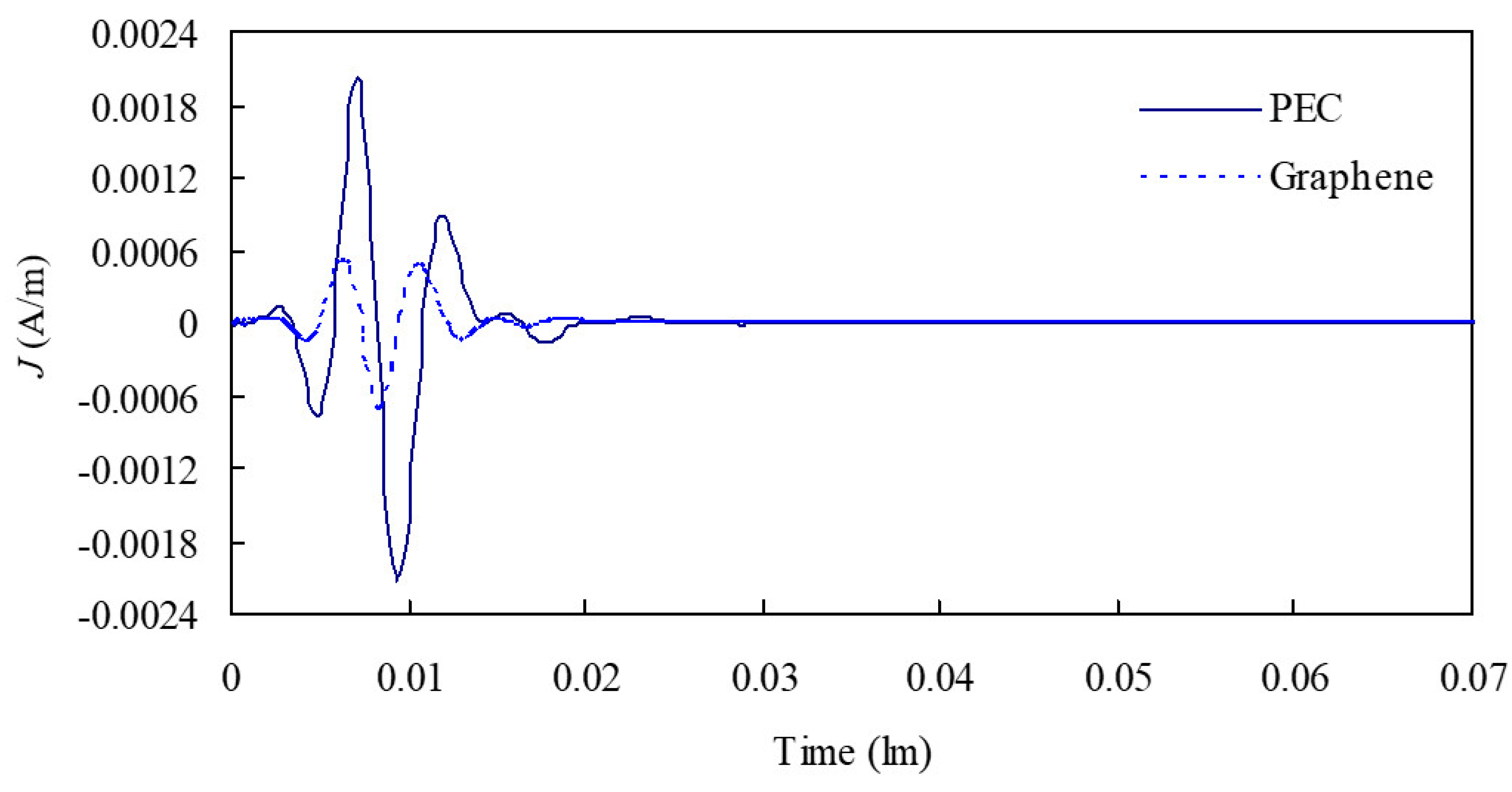
Two end points of a randomly chosen inner edge are (−0.413391 × 10⁻³, −0.254972 × 10⁻³, 0) and (−0.326874 × 10⁻³, −0.205698 × 10⁻³, 0). Current across this inner edge is shown in Figure 2. The dispersion of graphene leads to differences in comparison with the perfect electric conductor (PEC) plate of the same size. The unit of the lateral axis is light meter (lm). One light meter is the time that the EM wave propagates 1 m in free space. The current in late time is stable and converges to zero.
Wide frequency band information, e.g., bistatic radar cross section (RCS), is obtained after the Fourier transform. Examples are chosen at 0.102, 0.204, and 0.374 THz. The results show good agreement with those obtained via MOM in Figure 3.
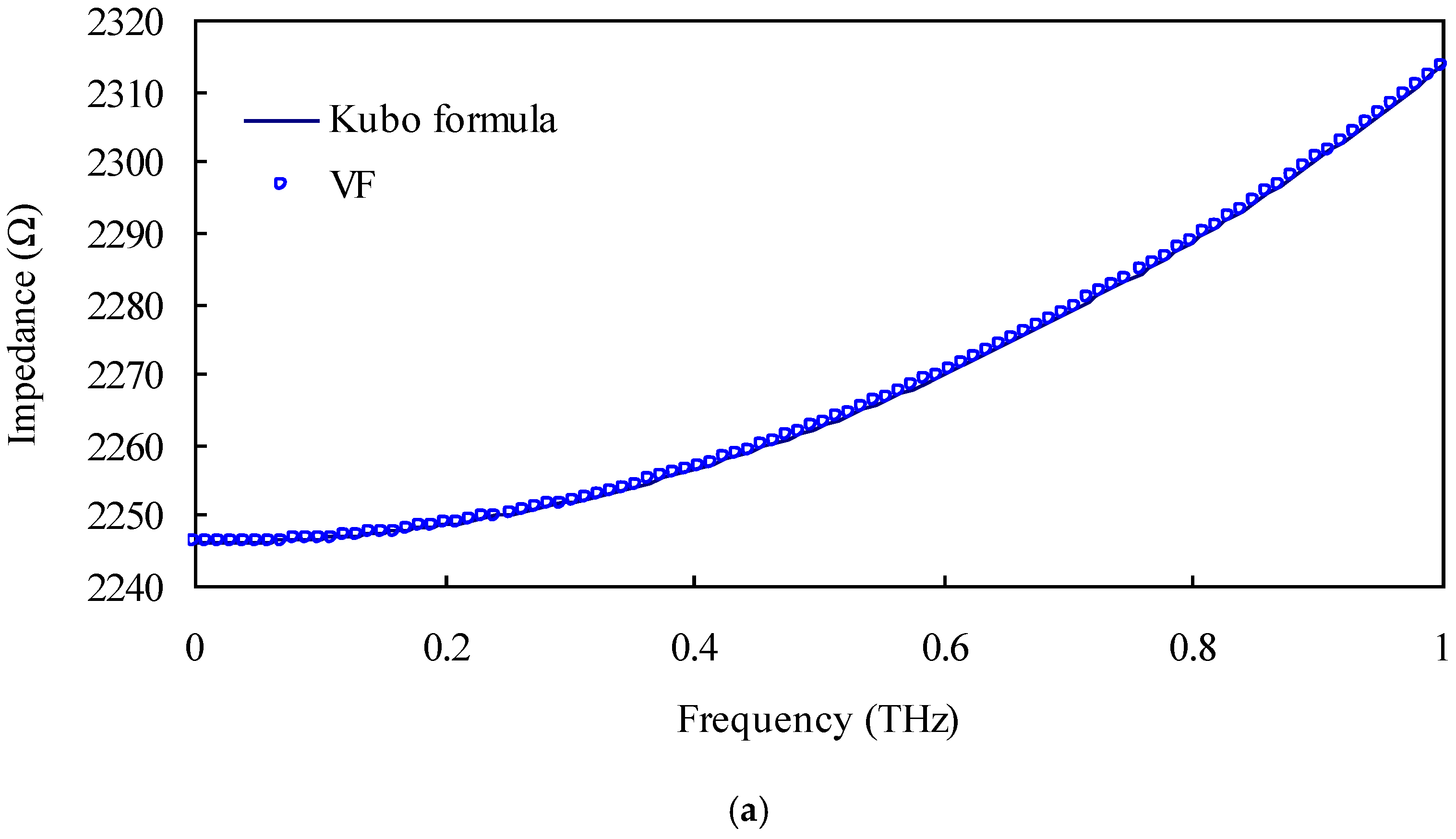
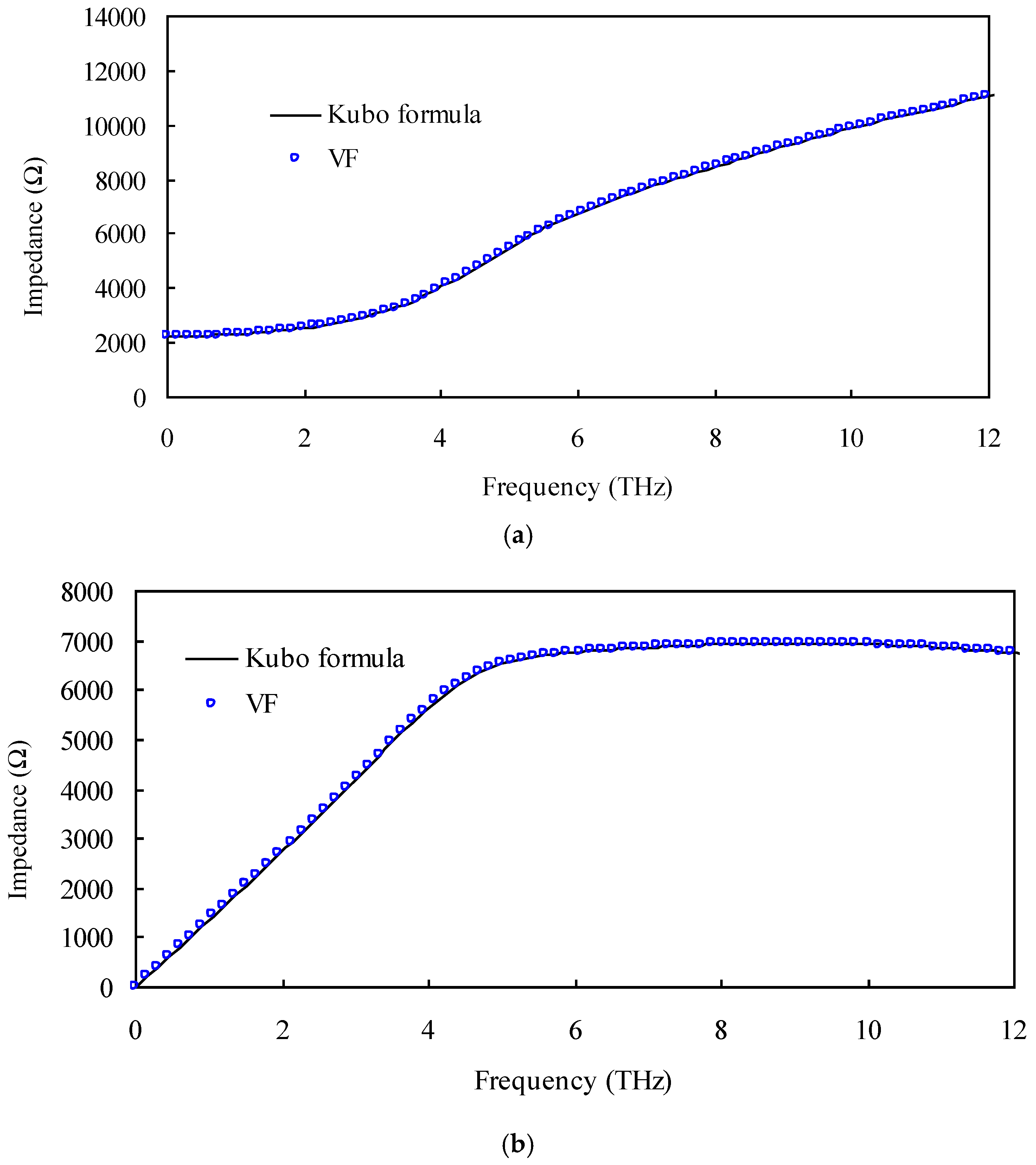
Another 12.5 μm × 25 μm (xoy plane) graphene sheet (μc = 0.01 eV, Γ = 5 × 10¹² s−1, T = 300 K) and frequency up to 12 THz are under discussion. The poles al and residues cl of graphene’s surface impedance computed with VF are listed in Table 2. Graphene’s surface impedances are computed and compared in Figure 4, where the results of VF agree well with those computed by the Kubo formula.
For graphene, the total-scattering cross section (TSCS), the absorption cross section (ACS), and the extinction cross section (ECS) are other interesting parameters. The ECS at frequency f is computed according to the electromagnetic optical theorem [35] as:
where Einc and Esca are the incident and scattering amplitude in the forward direction, and Im( ) is the imaginary part.
The graphene surface current is expressed by 123 RWGs and 80 WLPs. The scaling factor s is 3.6 × 10¹³. The ECS above 1 THz computed with MOD TDIE show good agreement with those obtained via MOM in Figure 5.
Based on the MOD TDIE solver developed in this paper, transient electromagnetic modeling of multilayer graphene with metallic and/or dielectric substrate will be studied with PMCHWT formulation in the future by the authors. The memory and time complexity of the standard MOD TDIE method are O (NS2NL) and O (NS2NL2), respectively, where NS is the number of inner edges, NL is the highest degree of WLPs. The memory requirement and computation time can decrease by combining fast algorithms or parallelization codes.
4. Conclusions
TDIE for the transient electromagnetic scattering of the graphene is solved following the MOD scheme. TDIE is established enforcing the surface impedance boundary condition. The convolution of the temporal surface impedance and current is deduced. The temporal surface impedance is obtained after the inverse Fourier transform of the frequency domain counterparts, which are approximated using the VF method. Stable and accurate solution can be ensured.
Acknowledgments
This work was supported by the National Natural Science Foundation of China (61501252, 61501159) and the Open Research Program of State Key Laboratory of Millimeter Waves of Southeast University (K201608, K201602).
Author Contributions
Quanquan Wang derived the formulation and wrote the paper; Huazhong Liu and Yan Wang performed the numerical simulation; Zhaoneng Jiang assisted in paper review.
Conflicts of Interest
The authors declare no conflict of interest.
References
- Warner, J.H.; Schäffel, F.; Rümmeli, M.; Bachmatiuk, A. Graphene: Fundamentals and Emergent Applications, 1st ed.; Elsevier: Oxford, UK, 2012. [Google Scholar]
- Balci, O.; Polat, E.O.; Kakenov, N.; Kocabas, C. Graphene-enabled electrically switchable radar-absorbing surfaces. Nat. Commun. 2015, 6, 6628. [Google Scholar] [CrossRef] [PubMed]
- Wan, T.H.; Chiu, Y.F.; Chen, C.W.; Hsu, C.C.; Cheng, I.C.; Chen, J.Z. Atmospheric-pressure plasma jet processed Pt-decorated reduced graphene oxides for counter-electrodes of dye-sensitized solar cells. Coatings 2016, 6, 44. [Google Scholar] [CrossRef]
- Zheng, G.G.; Zhang, H.J.; Bu, L.B. Narrow-band enhanced absorption of monolayer graphene at near-infrared (NIR) sandwiched by dual gratings. Plasmonics 2017, 12, 271–276. [Google Scholar] [CrossRef]
- Zhu, W.R.; Xiao, F.J.; Kang, M.; Sikdar, D.; Premaratne, M. Tunable terahertz left-handed metamaterial based on multi-layer graphene-dielectric composite. Appl. Phys. Lett. 2014, 104, 051902. [Google Scholar] [CrossRef]
- Thampy, A.S.; Darak, M.S.; Dhamodharan, S.K. Analysis of graphene based optically transparent patch antenna for terahertz communications. Physica E 2015, 66, 67–73. [Google Scholar] [CrossRef]
- Fallahi, A.; Perruisseau-Carrier, J. Design of tunable biperiodic graphene metasurfaces. Phys. Rev. B 2012, 86, 195408. [Google Scholar] [CrossRef]
- Chen, Y.P.; Sha, W.E.I.; Jiang, L.J.; Hu, J. Graphene plasmonics for tuning photon decay rate near metallic split-ring resonator in a multilayered substrate. Opt. Express 2015, 23, 2798–2807. [Google Scholar] [CrossRef] [PubMed]
- Shapoval, O.V.; Gomez-Diaz, J.S.; Perruisseau-Carrier, J.; Mosig, J.R.; Nosich, A.I. Integral equation analysis of plane wave scattering by coplanar graphene-strip gratings in the THz range. IEEE Trans. THz Sci. Technol. 2013, 3, 666–674. [Google Scholar] [CrossRef]
- Balaban, M.V.; Shapoval, O.V.; Nosich, A.I. THz wave scattering by a graphene strip and a disk in the free space: Integral equation analysis and surface plasmon resonances. J. Opt. 2013, 15, 114007. [Google Scholar] [CrossRef]
- Lin, H.; Pantoja, M.F.; Angulo, L.D.; Alvarez, J.; Martin, R.G.; Garcia, S.G. FDTD modeling of graphene devices using complex conjugate dispersion material model. IEEE Microw. Wirel. Compon. Lett. 2012, 22, 612–614. [Google Scholar] [CrossRef]
- Nayyeri, V.; Soleimani, M.; Ramahi, O.M. Wideband modeling of graphene using the finite-difference time-domain method. IEEE Trans. Antennas Propag. 2013, 61, 6107–6114. [Google Scholar] [CrossRef]
- Wang, D.W.; Zhao, W.S.; Gu, X.Q.; Chen, W.C.; Yin, W.Y. Wideband modeling of graphene-based structures at different temperatures using hybrid FDTD method. IEEE Trans. Nanotechnol. 2015, 14, 250–258. [Google Scholar] [CrossRef]
- Li, P.; Jiang, L.J.; Bağci, H. A resistive boundary condition enhanced DGTD scheme for the transient analysis of graphene. IEEE Trans. Antennas Propag. 2015, 63, 3065–3076. [Google Scholar] [CrossRef]
- Li, P.; Jiang, L.J. Modeling of magnetized graphene from microwave to THz range by DGTD with a scalar RBC and an ADE. IEEE Trans. Antennas Propag. 2015, 63, 4458–4467. [Google Scholar] [CrossRef]
- Li, P.; Shi, Y.F.; Jiang, L.J.; Bağci, H. DGTD analysis of electromagnetic scattering from penetrable conductive objects with IBC. IEEE Trans. Antennas Propag. 2015, 63, 5686–5697. [Google Scholar]
- Shi, Y.F.; Uysal, I.E.; Li, P.; Ulku, H.A.; Bağci, H. Analysis of electromagnetic wave interactions on graphene sheets using time domain integral equations. In Proceedings of the International ACES Conference, Williamsburg, VA, USA, 22–26 March 2015. [Google Scholar]
- Shi, Y.F.; Li, P.; Uysal, I.E.; Ulku, H.A.; Bağci, H. An MOT-TDIE solver for analyzing transient fields on graphene-based devices. In Proceedings of the IEEE International Symposium Antennas Propagation (APSURSI), Fajardo, Puerto Rico, 26 June–1 July 2016. [Google Scholar]
- Jung, B.H.; Chung, Y.S.; Sarkar, T.K. Time-domain EFIE, MFIE, and CFIE formulations using Laguerre polynomials as temporal basis functions for the analysis of transient scattering from arbitrary shaped conducting structures. Prog. Electromagn. Res. 2003, 39, 1–45. [Google Scholar] [CrossRef]
- Chung, Y.S.; Lee, Y.J.; So, J.H.; Kim, J.Y.; Cheon, C.Y.; Lee, B.J.; Sarkar, T.K. A stable solution of time domain electric field integral equation using weighted Laguerre polynomials. Microw. Opt. Tech. Lett. 2007, 49, 2789–2793. [Google Scholar] [CrossRef]
- Mei, Z.C.; Zhang, Y.; Sarkar, T.K.; Salazar-Palma, M.; Jung, B.H. Analysis of arbitrary frequency-dependent losses associated with conducting structures in a time-domain electric field integral equation. IEEE Antennas Wirel. Propag. Lett. 2011, 10, 678–681. [Google Scholar]
- Shi, Y.; Jin, J.M. Time-domain augmented EFIE and its marching-on-in-degree solution. Microw. Opt. Technol. Lett. 2011, 53, 1439–1444. [Google Scholar] [CrossRef]
- Shi, Y.; Jin, J.M. A time-domain volume integral equation and its marching-on-in-degree solution for analysis of dispersive dielectric objects. IEEE Trans. Antennas Propag. 2011, 59, 969–978. [Google Scholar] [CrossRef]
- Wang, Q.Q.; Liu, Z.W.; Shi, Y.F.; Zhang, H.H.; Chen, R.S. Efficient generation of aggregative basis functions in the marching-on-in-degree time-domain integral equation solver. Electromagnetics 2013, 33, 370–378. [Google Scholar] [CrossRef]
- He, Z.; Chen, R.S.; Sha, W.E.I. An Efficient marching-on-in-degree solution of transient multiscale EM scattering problems. IEEE Trans. Antennas Propag. 2016, 64, 3039–3046. [Google Scholar] [CrossRef]
- Valdes, F.; Andriulli, F.P.; Bağci, H.; Michielssen, E. Time-domain single-source integral equations for analyzing scattering from homogeneous penetrable objects. IEEE Trans. Antennas Propag. 2013, 61, 1239–1254. [Google Scholar] [CrossRef]
- Shi, Y.F.; Bağci, H.; Lu, M.Y. On the internal resonant modes in marching-on-in-time solution of the time domain electric field integral equation. IEEE Trans. Antennas Propag. 2013, 61, 4389–4392. [Google Scholar] [CrossRef]
- Shi, Y.F.; Bağci, H.; Lu, M.Y. On the static loop modes in the marching-on-in-time solution of the time-domain electric field integral equation. IEEE Antennas Wirel. Propag. Lett. 2014, 13, 317–320. [Google Scholar]
- Gustavsen, B.; Semlyen, A. Rational approximation of frequency domain responses by vector fitting. IEEE Trans. Power Deliv. 1999, 14, 1052–1061. [Google Scholar] [CrossRef]
- Gustavsen, B. Improving the pole relocating properties of vector fitting. IEEE Trans. Power Deliv. 2006, 21, 1587–1592. [Google Scholar] [CrossRef]
- Deschrijver, D.; Mrozowski, M.; Dhaene, T.; de Zutter, D. Macromodeling of multiport systems using a fast implementation of the vector fitting method. IEEE Microw. Wirel. Compon. Lett. 2008, 18, 383–385. [Google Scholar] [CrossRef]
- Romano, D.; Antonini, G. Partial element equivalent circuit-based transient analysis of graphene-based interconnects. IEEE Trans. Electromagn. Compat. 2016, 58, 801–810. [Google Scholar] [CrossRef]
- Zhao, P.; Wu, K.L. Model-based vector-fitting method for circuit model extraction of coupled-resonator diplexers. IEEE Trans. Microw. Theory Tech. 2016, 64, 1787–1797. [Google Scholar] [CrossRef]
- Parvaz, R.; Karami, H. Far-infrared multi-resonant graphene-based metamaterial absorber. Opt. Commun. 2017, 396, 267–274. [Google Scholar] [CrossRef]
- Mishchenko, M.I.; Travis, L.D.; Lacis, A.A. Scattering, Absorption, and Emission of Light by Small Particles; Cambridge University Press: Cambridge, UK, 2002. [Google Scholar]
Figure 1.
Graphene’s surface impedance: (a) real parts; (b) imaginary parts.

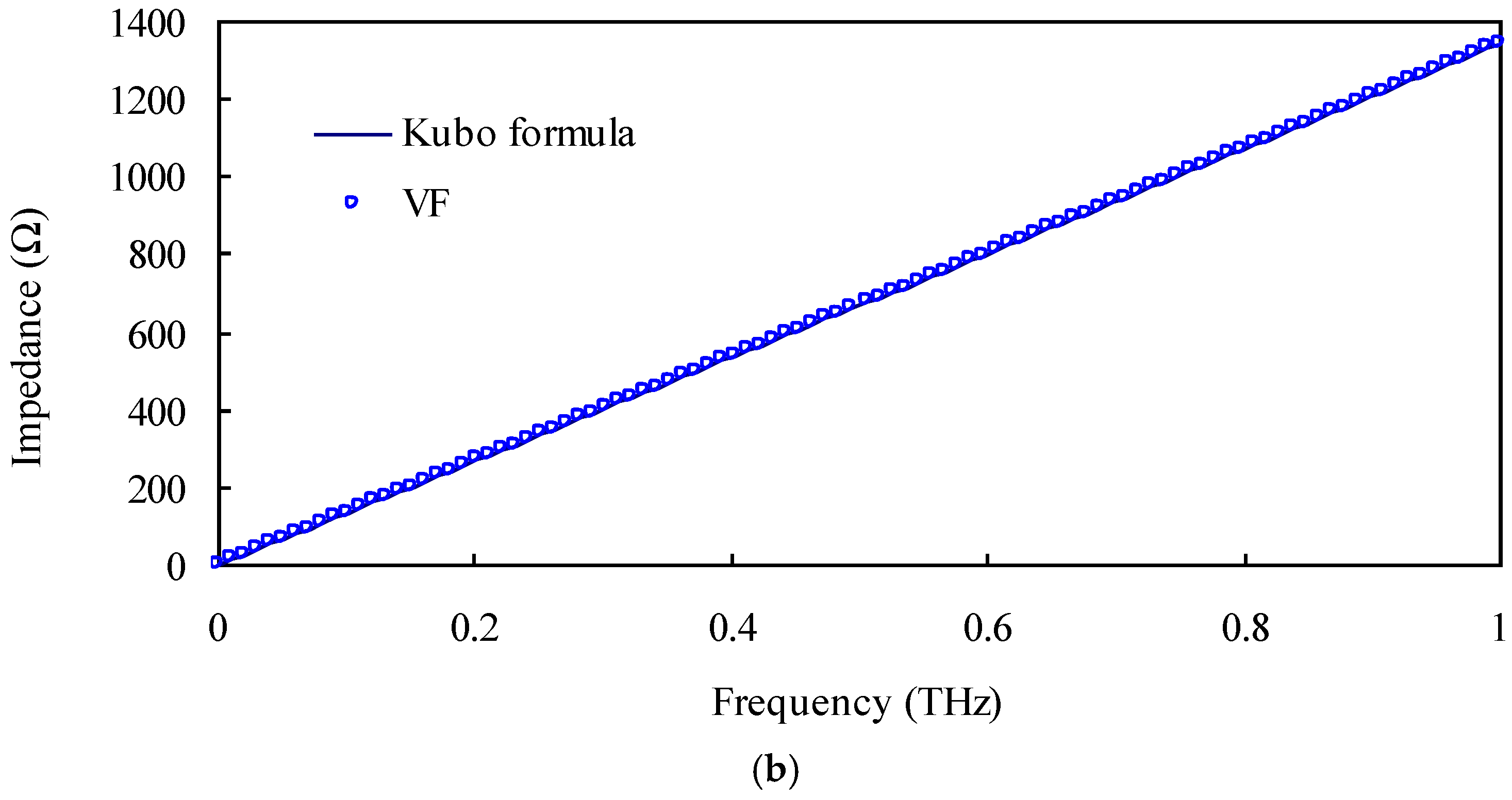
Figure 2.
Induced current across a randomly chosen inner edge of the graphene sheet.

Figure 3.
φ = 90° bistatic radar cross section (RCS) of the graphene sheet: (a) 0.102 THz; (b) 0.204 THz; (c) 0.374 THz.
Figure 3.
φ = 90° bistatic radar cross section (RCS) of the graphene sheet: (a) 0.102 THz; (b) 0.204 THz; (c) 0.374 THz.
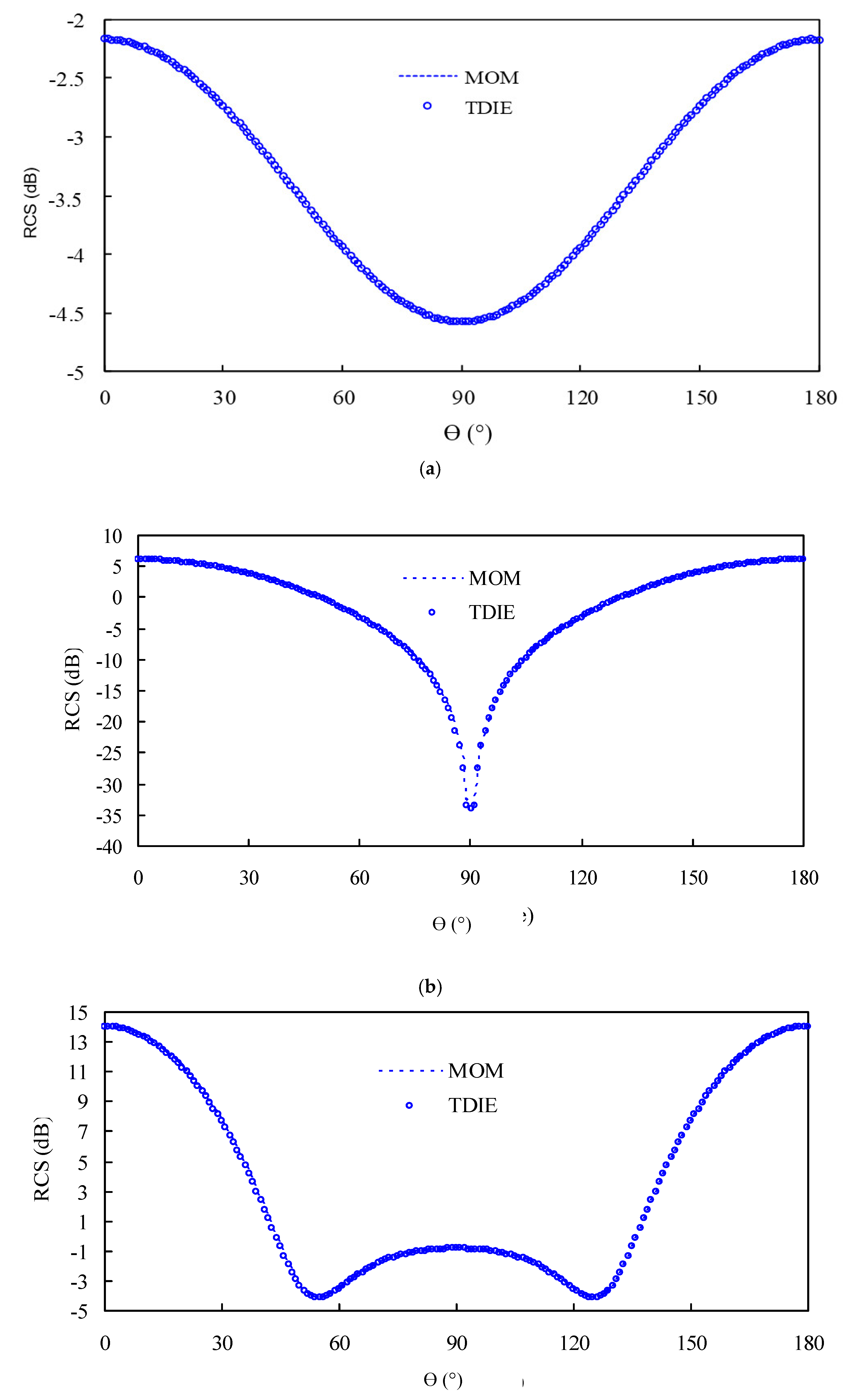
Figure 4.
Graphene’s surface impedance: (a) real parts; (b) imaginary parts.

Figure 5.
The extinction cross section (ECS) of the graphene sheet above 1 THz.


Table 1.
The poles al and residues cl when p = 2.
| l | al | cl |
|---|---|---|
| 1 | (–1.4148 + j6.8532) × 1013 | (5.5230 + j0.3378) × 1017 |
| 2 | (–1.4148 – j6.8532) × 1013 | (5.5230 – j0.3378) × 1017 |
Table 2.
The poles al and residues cl when p = 4.
| l | al | cl |
|---|---|---|
| 1 | –6.5249 × 10¹³ | –8.5729 × 10¹⁷ |
| 2 | –2.7141 × 10¹⁶ | 4.4980 × 10²⁰ |
| 3 | (–1.2248 + j2.6437) × 1013 | (–0.8148 + j1.5576) × 1016 |
| 4 | (–1.2248 – j2.6437) × 1013 | (–0.8148 – j1.5576) × 1016 |
© 2017 by the authors. Licensee MDPI, Basel, Switzerland. This article is an open access article distributed under the terms and conditions of the Creative Commons Attribution (CC BY) license (http://creativecommons.org/licenses/by/4.0/).
Share and Cite
MDPI and ACS Style
Wang, Q.; Liu, H.; Wang, Y.; Jiang, Z. Marching-on-in-Degree Time-Domain Integral Equation Solver for Transient Electromagnetic Analysis of Graphene. Coatings 2017, 7, 170. https://doi.org/10.3390/coatings7100170
AMA Style
Wang Q, Liu H, Wang Y, Jiang Z. Marching-on-in-Degree Time-Domain Integral Equation Solver for Transient Electromagnetic Analysis of Graphene. Coatings. 2017; 7(10):170. https://doi.org/10.3390/coatings7100170
Chicago/Turabian StyleWang, Quanquan, Huazhong Liu, Yan Wang, and Zhaoneng Jiang. 2017. "Marching-on-in-Degree Time-Domain Integral Equation Solver for Transient Electromagnetic Analysis of Graphene" Coatings 7, no. 10: 170. https://doi.org/10.3390/coatings7100170
Note that from the first issue of 2016, this journal uses article numbers instead of page numbers. See further details here.