Study of Near-Cup Droplet Breakup of an Automotive Electrostatic Rotary Bell (ESRB) Atomizer Using High-Speed Shadowgraph Imaging

Abstract

Electrostatic Rotary bell (ESRB) atomizers are used as the dominant means of paint application by the automotive industry. They utilize the high rotational speed of a cup to induce primary atomization of a liquid along with shaping air to provide secondary atomization and transport. In order to better understand the fluid breakup mechanisms involved in this process, high-speed shadowgraph imaging was used to visualize the edge of a serrated rotary bell at speeds varying between 5000 and 12,000 RPM and with a water flow rate of 250 ccm. A multi-step image processing algorithm was developed to differentiate between ligaments and droplets during the primary atomization process. The results from this experiment showed that higher bell speeds resulted in a 26.8% reduction in ligament and 22.3% reduction in droplet Sauter Mean Diameters (SMD). Additionally, the ligament (ranging from 40 to 400 μm) diameters formed bimodal distributions, while the droplet (ranging from 40 to 300 μm) diameters formed a normal distribution. Velocities were also measured using particle tracking velocimetry, in which size-dependent velocities could then be computed. Droplet velocities were affected more by rotational speed than droplet SMD, while ligaments were affected by other factors than the rotational speed and ligament SMD.

1. Introduction

Rotary bell applicators are one class of spray atomizers that use centrifugal forces to break up fluid. This system is used in various applications such as coating applicators, fuel injectors, mass spectroscopy, drug delivery, and pesticide application [1,2]. However, one challenging application is in automotive painting due to the production rate, size of the vehicle, environmental impact, fluid properties and the importance of droplet size uniformity and film build consistency on the appearance and finish of the vehicle [3,4]. Rotary bell (or cup) applicators operate by releasing fluid along the center of a rotating cup, which forms a thin liquid film over the inner surface of the cup. When the film reaches the edge of the cup, ligaments (connected liquid threads) are formed. Air flow around the outside of the cup, referred to as shaping air, contributes to additional liquid breakup into droplets and directs the droplets towards the target, thus resulting in application of the fluid to a substrate. In the automotive industry, the paint is often electrostatically charged to enhance the transfer of the paint to the target [3,5].

Rotary bell atomizers have been the primary method of paint application for many manufacturers due to the increased paint transfer efficiency over the alternative of air spray guns, such as air blast sprayers. However, the devices leave room for improvement since over-coating is often necessary to ensure sufficient finish quality [5,6]. Since its inception into industry, rotating disk, and later rotary bell, applicators have been studied in an attempt to understand and improve the paint application process, but further improvements would continue to reduce costs and waste in industrial processes. Currently, automotive paint shops amount to 30%–50% of the total cost to manufacture automobiles and up to 70% of the total energy costs in an assembly plant [3,5]. Thus, even small improvements to any aspect of the process is important, since it can result in large cost savings and waste reduction.

One of the most often-studied aspects of rotary bell and rotating disk applicators has been the atomization process. Early studies led to the fundamental physical interpretation of liquid atomization in these systems [7,8,9,10], where it was found that the atomization process begins with thin ligaments forming at the edge of the bell that eventually breakup into droplets. Particle size distributions for droplets were also found to be Gaussian with a slight skew toward smaller sizes. Liquid breakup from the ligaments has also been described, including laminar breakup of single jet ligament length [11], jet breakup time characterization [12], and liquid ligament detachment/elongation characterization [13].

Spinning disk applicators have similar flowfield characteristics as the bell spray process, clearly showing the ligament and droplet formation. Many studies have been conducted with regards to the critical parameters and characteristics of spinning disk and wheel applications, such as ligament and droplet formation and droplet size distributions [14,15,16,17,18,19]. Notable observations from spinning disk literature include that the Sauter mean diameter increases with decreased rotational speed [15], and that velocity slip of the liquid film flowing over a rotating wheel is significant when the wheel rotation is slow but is negligible at high Weber numbers [17]. Additionally, spinning disks with teeth or serrations [18] had a characteristic bimodal droplet size distribution, which was notably different from the typical polydispersed distribution for flat-rimmed rotating atomizers [15].

Many studies have been performed to characterize the effects of various parameter changes on atomization, including flowrate, rotational speed, and cup geometry with regards to bell atomizers [20]. Experimental [6,16] and simulated parametrization [21] have both been conducted and it was found that increasing the flow rate of rotary atomizers leads to a transition from aerodynamic (or jet) disintegration to turbulent disintegration of the ligaments, whereby there is a transition of ligament formation to sheet formation at the cup edge [4,22]. Increasing rotational speed was observed to result in less homogeneous disintegration [4]. Additionally, the droplet size distribution near the cup showed multi-modal shapes at low rotational speeds with [6] and without the inclusion [22] electrostatic forces. It has been suggested that the spray is dominated by main and satellite drop sizes, corresponding to the peaks in the number distributions. Such bimodal distributions affect the final appearance [23] and the transfer efficiency [3]. The bimodal distributions have been shown to converge to a single mode with increasing RPM as well.

There have also been a variety of techniques used in imaging and determining droplet sizes for general sprays. Laser diffraction (LD) is the most common form of droplet sizing in sprays [24]. The method quantifies the droplet size distribution over a wide range through the spray flowfield (plume). Though it does not give other flow properties such as velocity, other methods such as Phase Doppler Anemometry (PDA) and Phase-Doppler Particle Analyzer (PDPA) overcame that flaw and measure properties such as droplet-size distribution, velocity, density, and mass flux [15]. Another viable imaging technique is shadowgraph imaging, where captured images require further processing to determine the sizes of droplets and ligaments [25,26,27], but provide accurate statistics after calibration.

In addition to droplet and ligament size information, velocities of the fluid particles are of particular interest in understanding the transfer of the droplet cloud to the substrate. Particle image velocimetry (PIV) is a technique that can be used to determine velocity fields and has been investigated in previous spray studies to measure the velocity of flow fields and individual droplet velocities [28,29]. However, this technique does require two consecutive frames in time so that the particles can be correlated to produce the velocity vectors. This can be done through laser-pulse imaging and with high-speed cameras. It is worth noting that PIV and micro-PIV have been used in rotary bell atomization to measure the shaping air velocity and the droplet velocity in the flow field [30,31,32,33]. To our knowledge, there are no archival articles that reported the near cup droplet and ligament velocities using PIV methods. Thus, measured velocity statistics could provide meaningful new data. PIV in conjunction with particle tracking velocimetry (PTV) was used in the present work, with a high-speed camera, to calculate the near-cup ligament and droplet velocities.

Direct droplet and ligament formation, as well as droplet sizing, have been investigated in various capacities for rotary bell applicators. However, these studies were not conducted with the inclusion of shaping airflow [22,23,34,35], which is used in the automotive industry for paint application. While general research into pulsed airflow breakup effects [36] and specific study of rotary bell atomization characteristics with shaping air [37] have been conducted, the combination of studying droplet and ligament size evolution with changing parameters in the near field has not been reported. Additionally, many studies examine the atomization process with the inclusion of electrostatic forces [7,38], which show droplet size distributions are bimodal.

This paper examines a rotary bell applicator near the cup with shaping air using a high speed shadowgraph imaging setup. While the technique itself has been used, its use for near-field imaging of rotary bell applicators to capture fluid particle size and simultaneous velocity measurements has not been reported in literature. The purpose of this work was to develop an imaging technique that could examine the physical breakup mechanisms at high rotational speeds, gain meaningful size and velocity statistics, and correlate the size and velocity data from individual fluid particles, all from a single data set. This was accomplished by utilizing high-speed shadowgraph imaging and several image processing techniques to eliminate some of the inherent background noise that accompanies this type of atomization. Ultimately, this work adds valuable insight into the study of the atomization process and aids in increasing paint transfer efficiency by demonstrating a new measurement technique for studying near-field atomization and presenting meaningful fluid particle data by using this technique.

2. Materials and Methods

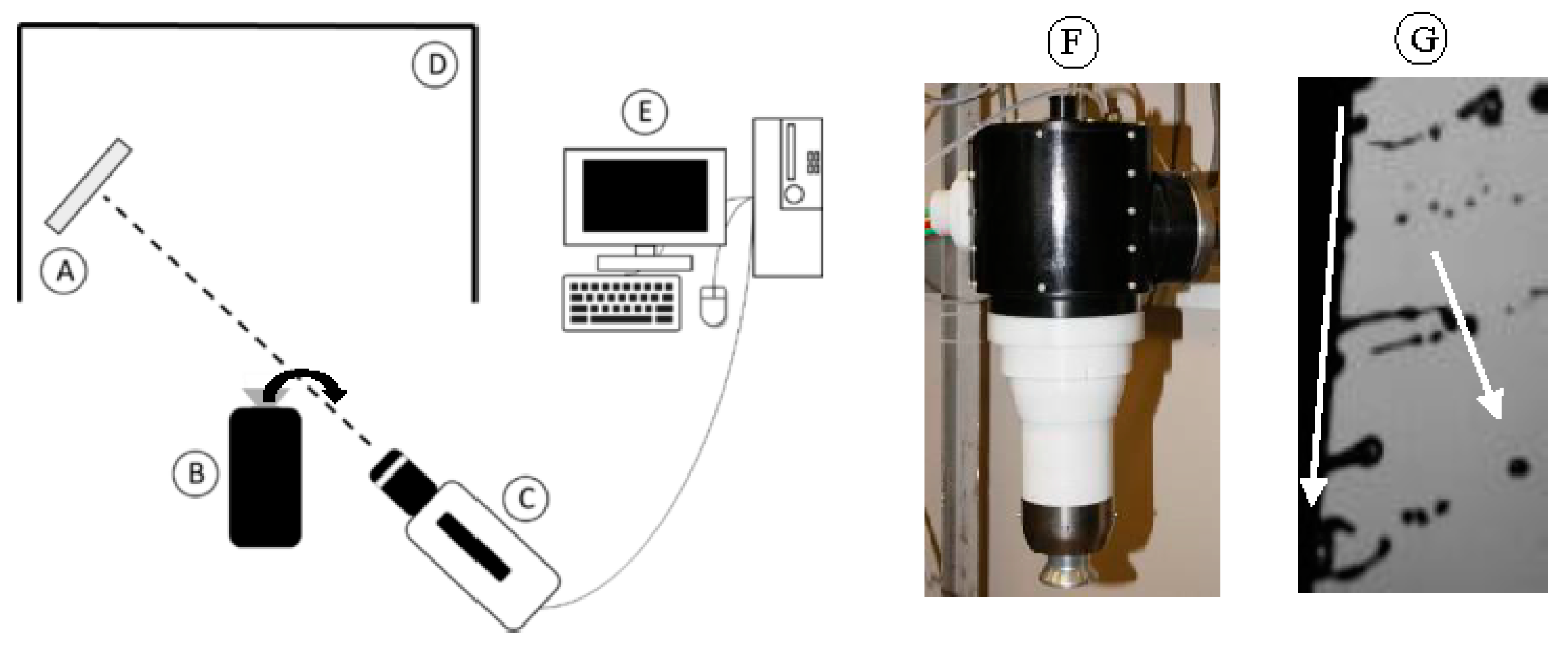
2.1. Experimental Setup

An ASEA Brown Boveri Ltd. (ABB, Zürich, Switzerland) rotary bell atomizer, seen in Figure 1 equipped with a 65 mm diameter serrated bell-cup was used in this experiment. The rotary bell was operated at speeds of 5000–12,000 RPM in intervals of 1000 RPM. Only rotational speed was varied in this experiment due to it being the dominant parameter in producing different droplet diameters for rotary bell atomizers utilizing water at the speeds conducted here [10]. Additionally, in another unpublished experiment, at higher rotational speeds and with multiple flow rates considered, a 96% dependence of droplet diameter on rotational speed was found with a two-way ANOVA (Analysis of Variance) analysis. Given these results, significant changes were only expected to be seen with variation in the rotational rate.

Liquid water (paint surrogate) was used as the atomization fluid and was sent through the bell at a flowrate of 250 ccm. The water released from the bell was contained within a side-draft paint booth. Additionally, the use of water, instead of paint, still allows for results that are relevant for automotive paint spray systems due to the similarity in Ekman numbers, which relate viscous and Coriolis forces in a system. The automotive industry operates at very high rotational speeds (>60,000 RPM), and with paint at viscosities around ten times larger than that of water at the rotational speeds used. This is proportionally compensated for in this experiment with the choice of reduced rotational speeds on the same order as the reduction in viscosity.

A 500 W lamp was used as the illumination source for shadowgraph imaging. A Phantom V611 CMOS camera (Vision Research, Wayne, NJ, USA) equipped with an f = 105 mm Sigma (Tokyo, Japan) lens was used to image the liquid. The illumination source and the camera were placed on opposing sides (transmission mode) of the rotary bell as shown in Figure 1. The acquisition rate of the camera was set to 340 kHz using 64 × 128 pixels with a spatial resolution of 25.9 μm/pixel, resulting in an overall field of view of 1.68 mm × 3.36 mm.

High-speed shadowgraph imaging was performed at the near field of the cup edge with the camera placed at an angle behind the cup to capture the ligament formation. The angle was chosen such that the entirety of the ligaments would be approximately perpendicular to the camera and most of the fluid in the image would be in this single plane, thus allowing the shadowgraph images to give more accurate sizes of the fluid particles. Shadowgraph imaging allowed the approximate edges of the water droplets to be identified. For each bell speed case, 150,000 consecutive images were taken, which amounts to approximately 441 ms of real-time acquisition, or nearly 37 full cup rotations for the 5000 RPM case. The images were then processed to determine size and velocity distributions.

It is also worth noting that this method was applied to water as opposed to paint. This is an indication of its effectiveness because of the fact that it is easier to image paint using shadowgraph than it is with water for a couple of reasons. Those reasons being that paint is more opaque and much more viscous than water. Therefore, the droplets have clearer edges in the images and much slower breakup times, assuming all operational parameters are equal. It can be assumed that the resulting shadowgraph data would also be easier for the image processing method presented as well.

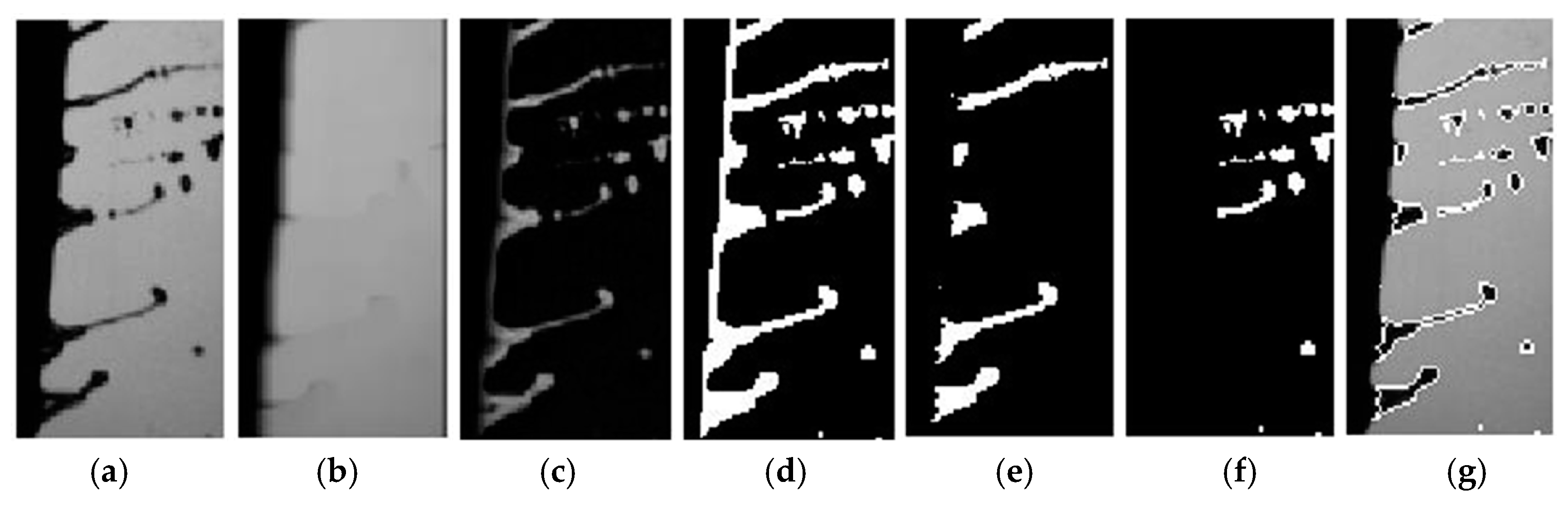
2.2. Image Processing

In order to process the images for both droplet and ligament size statistics, a processing algorithm was used to first identify liquid by binarizing the image, then connected liquid pixels were formed into groups, and finally segmented into either ligaments or droplets. An example of one of the raw images can be seen in Figure 1, minus the direction arrows, and a visual representation of the image processing is shown in Figure 2. Typically, background images are needed to distinguish between signal and background noise levels. Unfortunately, the background signal differed image-to-image since the light source travelled through the droplet cloud, which varied between cases, before illuminating the near cup liquid, therefore an approximation for the background light signal was needed. Using MATLAB R2016a, a pseudo-background image was calculated as shown in Figure 2b (with the original raw image in Figure 2a). The background was computed by dilating [39] the original image with a horizontal line structuring element to suppress the individual liquid droplets that occur on small spatial scales and accentuate any larger scale variation in background light that varies frame-to-frame. The background light changes due to different amounts of particles passing between the focus plane of the camera and the illumination source. Once the background image was calculated, it was then subtracted from the original image to show only light that was refracted, and therefore showing only the liquid, shown in Figure 2c. Finally, this image was binarized using a static thresholding method after determining that adaptive thresholding methods, such as Otsu’s method, did not accurately predict the threshold necessary to yield an image containing only fluid elements. The thresholding point that did yield the isolated fluid element images did not significantly change across images, and so a static threshold was chosen that gave an image of only liquid consisting of both ligaments and droplets, as shown in Figure 2d. Afterwards, the outline of the processed image was superimposed on the original to check the accuracy of the processing, shown in Figure 2g. Once it was determined that the edges were sufficiently captured, the method was used for the remaining images.

The images were further processed to separate the ligaments from droplets. To do this, ligaments were defined as connected fluid elements attached to the cup and droplets as any other identified liquid in the image. Connected components, with eight-neighbor connectivity, were identified in the binarized image. The eight-neighbor connectivity in this case referring to the inclusion of the eight pixels that surround or “neighbor” every pixel in a 3 × 3 block through horizontal, vertical, and diagonal connection. This identification meant that the ligaments and the cup from the binarized image would be taken as a single object. The largest connected component was removed from the image, since it was always the combination of the cup and ligaments attached to the cup, leaving only the droplets in the image. The largest component was then placed in its own separate image, isolating the ligaments and cup edge, and the cup edge was subsequently removed from the new image using a circular fit from the original image. All of the pixels on the edge of and inside of the arc fit were set to zero, eliminating the entirety of the cup from the image. Following the cup removal, two images that could be used to determine size statistics remained, one with ligaments only (Figure 2e) and the other with droplets only (Figure 2f). The combination of the statistics gained from these two images was also considered and is henceforth referred to as “combined” or “overall” statistics.

Additionally, the length and width of ligaments were calculated from the processed images. Ligament widths were calculated by taking the width of each ligament at the cup edge. Ligament lengths were calculated by using a skeleton operation [39] that approximated the ligaments as a line with a width of one pixel, and then obtaining the length of the resulting lines. Thus, the widths can be thought of as ligament base widths and the lengths can be thought of as the length of the ligament beginning at the cup. The ligament lengths and widths were calculated to further investigate general changes in ligament geometry with rotational speed.

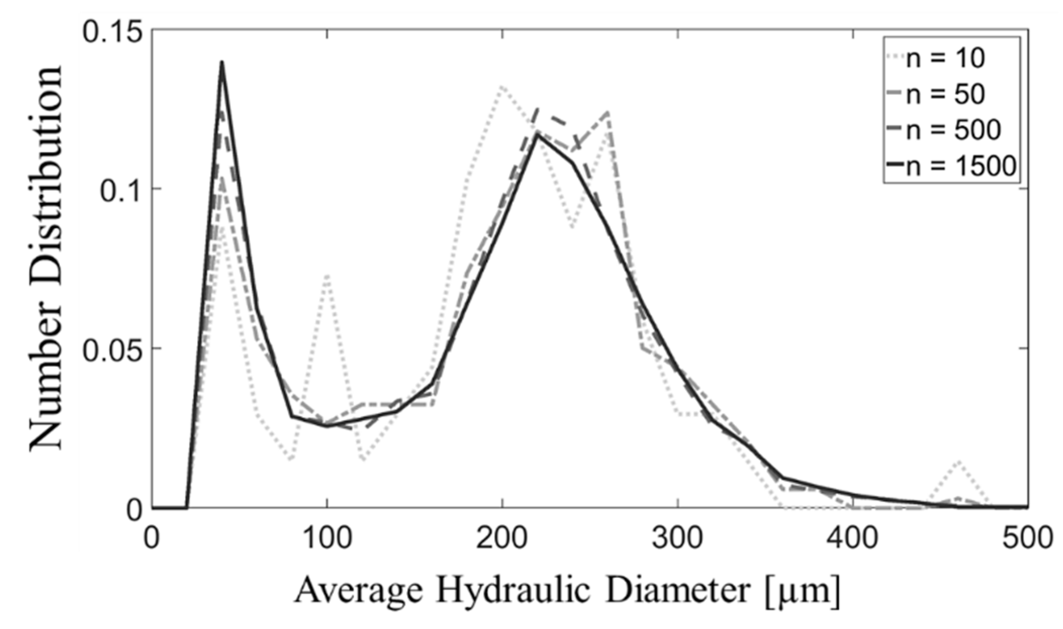
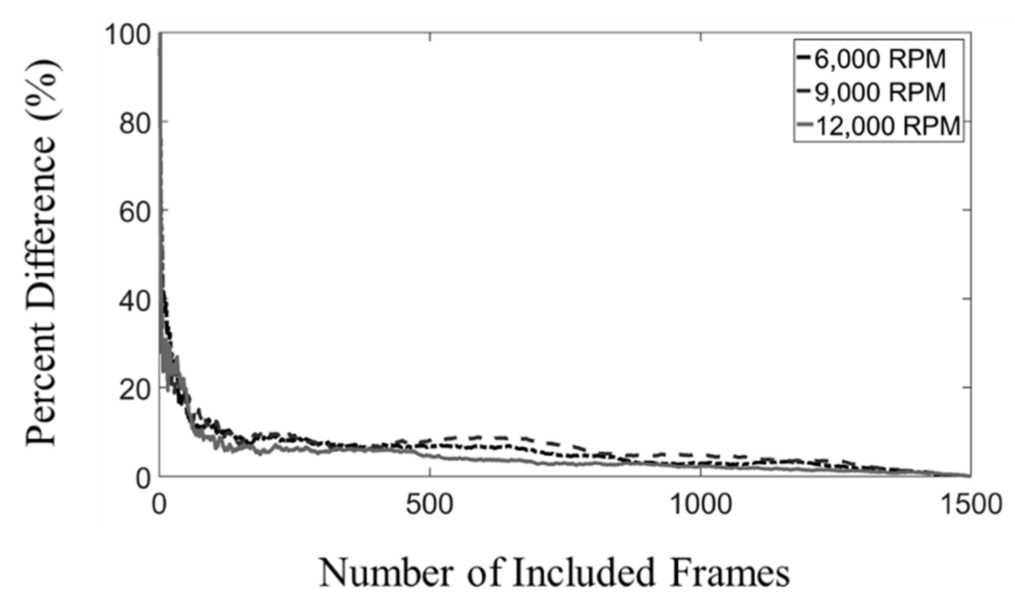
2.3. Size Measurements

Once the liquid was identified, fluid size statistics were next calculated. Fluid size was measured in terms of hydraulic diameter, calculated using Equation (1):

$$D_{\mathrm{h}}=\frac{4A}{P}$$

(1)

where D_h is the hydraulic diameter, A is the area of the object and P is the perimeter. The area of each droplet was defined as the pixel count of that group, and the perimeter as the number of pixels bordering the inscribing area for each individual droplet. The area and perimeter in pixels were converted into physical distance using a calibration to characterize the optical resolution. In order to get statistically different images of the liquid flowing from the bell, every 100th frame of the data was used, as this approximated a single flow time through the field of view in the 5000 RPM case. 1500 images were then used to determine the size statistics. Number distributions were then tabulated based on the resulting hydraulic diameter measurements. Volume distributions were also calculated by cubing the hydraulic diameters, which created a more size-weighted interpretation of the data.

To ensure that this sample size for these measurements was adequate, convergence tests were performed. This was done by calculating a size distribution, from a subset of the total 1500 measurements, and computing the percent difference between this subset statistic and that for all of the 1500 measurements. A subset, as used here, refers to taking the distribution from only a portion of the 1500 images, starting with one image. Progressively more data, in increments of one image, were added until the distribution of the collective subset of the original 1500 images was approximately that of the distribution when all of the images were included. At this point, the distribution required no more data to better represent the process and the distribution were said to have converged. Figure 3 shows the evolution of a single size distribution as more data was included and Figure 4 represents the percent difference evolution for three of the cases to further illustrate the convergence of the distributions. Ultimately, in the worst-case scenario, the distributions converged to less than 5% difference from the final distribution after approximately 700 frames were included in the data set. Thus, the distributions were taken as statistically converged. The frames at which each of the cases converged can be seen in

Table 1. The percentage of data (out of 1500 frames) at which the number distributions for size and velocity reach less than 5% difference compared to the final distribution (which includes the data from all 1500 images) for ligaments, droplets, and their combined (both ligaments and droplets) statistics at each bell speed tested.

Measured Quantities		Bell Speed [kRPM]
		5	6	7	8	9	10	11	12
Size	Ligaments	31.8	48.9	33.3	5.87	56.5	25.3	23.9	32.1
	Droplets	3.67	5.13	1.73	8.33	1.47	2.13	1.87	2.40
	Combined	3.87	7.40	5.67	8.00	4.07	3.13	1.87	2.53
Velocity	Ligaments	25.9	21.6	22.6	38.0	45.8	44.9	35.1	47.4
	Droplets	25.8	27.5	21.2	12.6	10.5	14.9	9.47	7.53
	Combined	17.4	17.1	14.9	6.07	7.80	13.0	5.13	6.60

.

2.4. Velocity Measurements

Davis 8.3 (LaVision, Ypsilanti, MI, USA) was used to obtain velocity information of the individual ligaments and droplets using combined PIV and PTV. The PIV algorithm utilized a multi-pass cross-correlation algorithm that successively worked down from 64 × 64 to 4 × 4 pixel interrogation window sizes with 50% overlap. The results from this process were velocity vector fields for the entire frame. The PTV option subsequently detected droplets in the image and reoriented the interrogation window to obtain a single vector for each droplet, discarding the remaining vectors in the velocity field. When post processing the data, if there were multiple vectors on a single droplet, the average of the velocity vectors was taken, and that data was subsequently used in the resulting velocity statistics. Using the combination of PIV and PTV, not only were droplet and ligament velocities able to be obtained, but the velocity vectors could also be correlated to the droplet and ligament sizes. 1500 evenly spaced sets of two sequential images in time were used for velocity calculations.

Statistical comparisons were done on one case to verify how many images were needed for the velocity distributions to converge, in the same manner as for the sizes, and it was found that the distributions converged to a less than a five percent difference from the final distribution after, in the worst case, 700 frames. This result can be found in Table 1, which shows the frames at which the velocity distributions converge to less than 5% difference. Thus, the 1500 sets of images are statistically converged for both size and velocity. The spacing between image sets was the exact same as for the size statistics, with the first image in each velocity image set corresponding to the same image used to determine sizes. This was done so that the velocity and size statistics could be directly correlated.

3. Results and Discussion

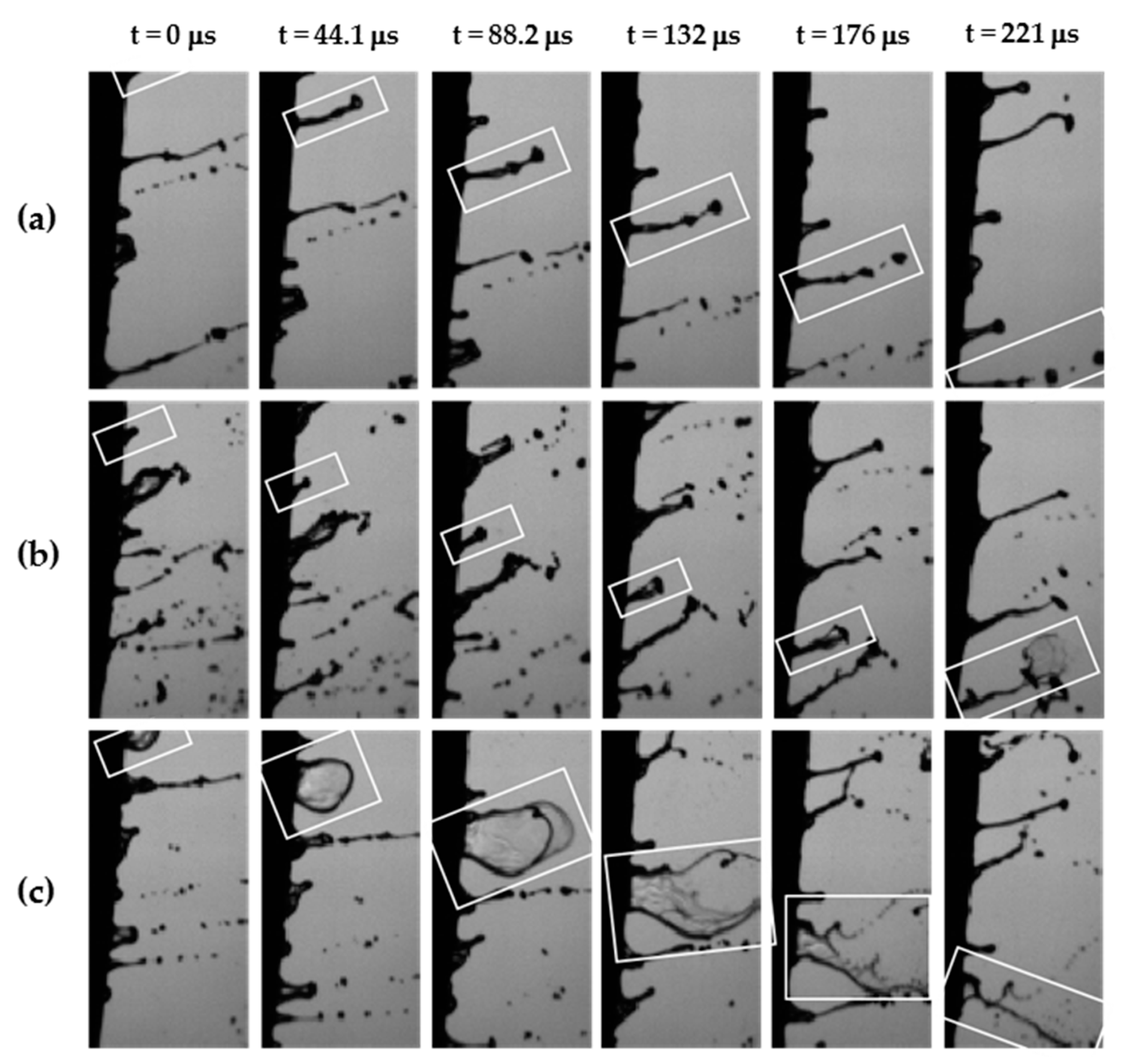
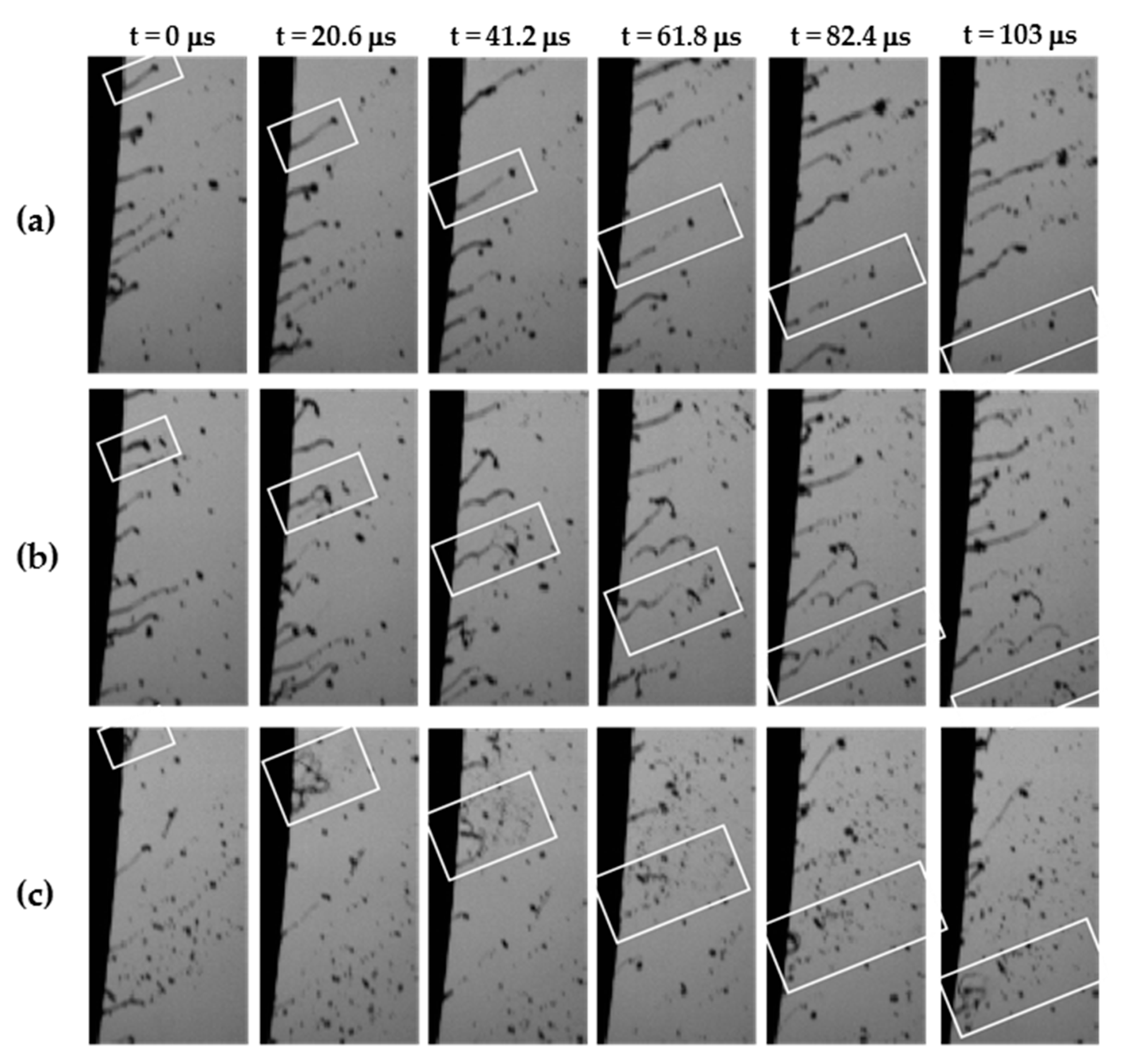
3.1. Ligament Breakup Observations

Unprocessed, consecutive experimental images were examined prior to any image processing to examine the ligament breakups for the various speeds. The raw image data was able to give information about the various fluid structures and ligament geometries that form at the edge of the cup. Combined with the high speed camera capability, detailed evolution of these structures over time was observed, as well as various fluid breakup and droplet formation mechanisms. Given that multiple rotational speeds were tested, the change in these mechanisms under additional shearing force was also observed. The observations of the ligament breakups at the 5, 8, and 12 kRPM are detailed in this study.

For the lowest rotational speed tested, 5 kRPM, there appear to be three typical regimes of fluid breakup, which can be seen in Figure 5. The first regime (shown on the row “a” of Figure 5) appears as an elongated ligament that holds a large volume of fluid at its unstable, mushroom-tip that subsequently breaks off into a droplet. The ligament in this case forms a wave along its length, likely due to Kelvin and Rayleigh instabilities, and then breaks up into smaller satellite droplets along its length in addition to the droplet it forms at the tip. The necking or pinching is typical of a Rayleigh breakup and indicates that another force, in this case the centrifugal force, has exceeded the surface tension force. This regime closely resembles the low momentum, thick ligament growth with multiple sequential breakups in Rao et al. [40].

A second regime that often appears is shown in the row b of Figure 5. The sequence begins with a standard long and thin ligament that initially forms with a larger fluid structure at the tip of the ligament, which subsequently breaks up into smaller droplets. The fluid structure at the tip rapidly expands, similar to a bag breakup [41,42], as opposed to the first regime which separates the entire fluid element. In a less frequent manner, a third regime, shown in the row c of Figure 5, appears and forms a ligament off the cup with a different structure. The ligament appears to be a translucent ring shape in the view of the camera, and is likely a thin-filmed ligament. The structure expands until the end of the liquid structure bursts into much finer droplets. Both the second and third observed breakup regimes resemble similarities to the standard bag breakup regime.

In the 8 kRPM case, seen in Figure 6, the ligaments are shorter and the droplets formed have smaller diameters than in the 5 kRPM case, as expected. The breakup, as a result, occurs closer to the edge of the cup, which indicates shorter breakup times. The ligament angle in relation to the cup also experiences a notable increase, which then translates into a change in the projection angle at which the droplets are ejected from the ligaments. This result is expected as well since the only change was rotational speed, which would thus increase the shearing force on the ligaments. Additionally, the same regimes that appeared in the previous case are observed to appear in this case. However, the elongated ligament to droplet breakup (row “a” of Figure 6) appears more prevalent and breaks up into more droplets along its length. The other notable difference is that the breakup in the row “c” of Figure 6 also resembles the bag-stamen type of breakup [41] as opposed to only a bag breakup.

Finally, in the 12 kRPM case, seen in Figure 7, the ligaments and droplets again become even smaller and disintegrate faster. The angle between the ligaments and the cup increases further still, and all of the mentioned regimes are still present. Additionally, the two forms of bag breakup (row “b” and “c” of Figure 7) appear even less frequently as the elongated ligament into droplet breakup (row “a” of Figure 7) becomes more dominant. The elongated ligaments also break into even more droplets along the ligament length than in the 8 kRPM case. Another observation is that the second type of breakup, seen in the row “b” of Figure 7, possibly transitions to a dual-bag breakup [43] and that the breakup sequence in row “c” may transition from bag-stamen to shear-stripping breakup [41]. Such results indicate that droplet formation modes, which normally occur in secondary breakup regions, are occurring in the primary breakup region in this process. They also indicate that the increasing difference in shearing force versus surface tension forces is advancing the type of breakup to smaller droplet sizes. All of these trends are continuations of the changes from the 5 to 8 kRPM case and can be said to be trends of the system as a whole under the conditions tested.

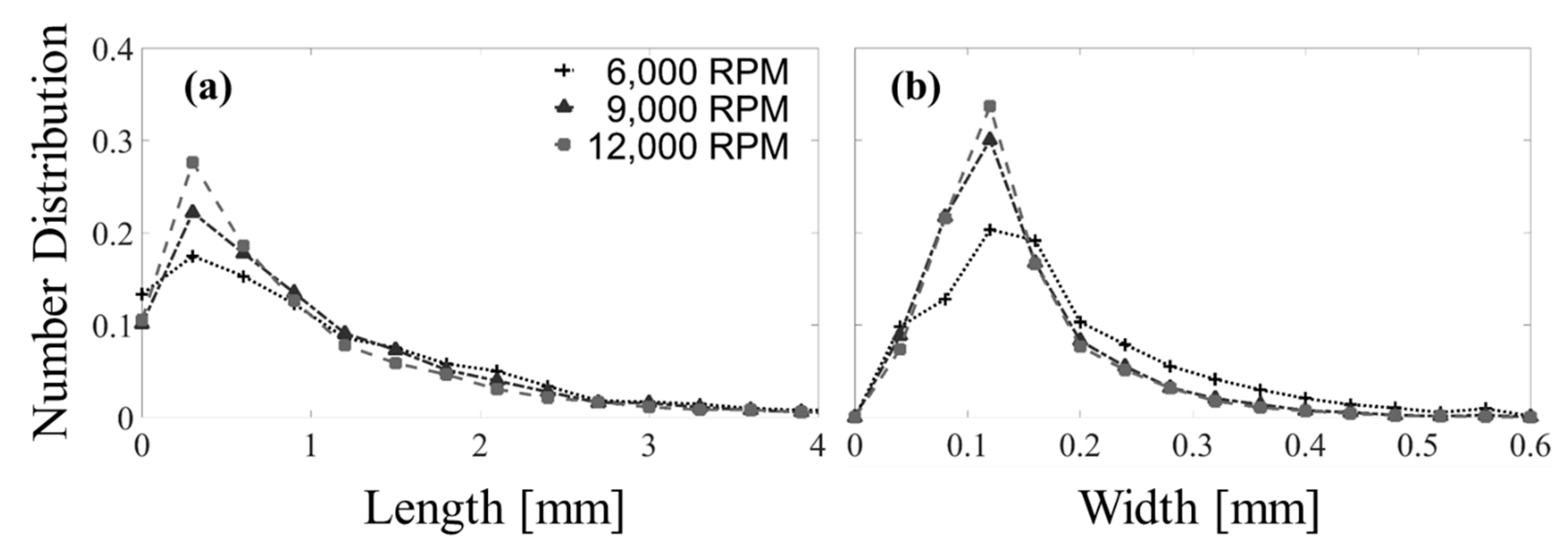
3.2. Size Statistics

The number and volume distributions for the ligaments and droplets, both separately and combined, are shown in Figure 8. These distributions were calculated by binning the hydraulic diameter statistics in 20 μm intervals and then normalizing the curves by the sum of the distribution. For the ligaments-only and droplets-only data, it is worth noting that the sum of overall distribution, which includes the data for both, was used instead of their respective sums. This normalization was done to show the relative contribution of the ligaments and droplets to the overall distribution. The droplets dominate the shape of the overall number distribution curve, which is expected since on average there are considerably more droplets in a given image than ligaments. Thus, an expanded version of the ligament number distribution was inset to better display its shape.

The number distributions show a shift for the droplets-only (Figure 8b), ligaments-only (Figure 8c) and overall (Figure 8a) distributions to smaller hydraulic diameters with increasing RPM. This trend is accentuated in the respective volume distribution graphs for the ligaments-only (Figure 8f), droplets-only (Figure 8e) and in the overall case (Figure 8d). The ligaments-only number distribution, shown in Figure 8c, is bimodal with a peak at larger hydraulic diameters shifting towards lower hydraulic diameters with higher RPM. The droplet-only distribution, shown in Figure 8b, shares a similar peak-shift to lower hydraulic diameters, but is not bimodal. These results collectively indicate that there are two regimes of ligament size in the near-cup field of view that lead to a single distribution of droplet sizes. Both ligament and droplet sizes decrease with increasing RPM.

It is worth noting that the peak at smaller hydraulic diameters for this data occurs near the resolution limit of the optical setup. Thus, any change in the diameters of these small particles with RPM is not resolved. The percentage of particles in this peak increases, without shifting, until the 12,000 RPM case where the particles are small enough to avoid being detected by the image processing. Such a result can be seen in Figure 8c, where the ligament distribution experienced a large reduction in small particle data. Additionally, despite the exclusion of electrostatic forces, the bimodality of the distributions is a result that matches what is found in the literature for electrostatic droplet size distributions [6].

The shapes of these droplet distributions are consistent to what is reported in literature, however, the ligaments have never been measured in this way, with a hydraulic diameter approximation. With the documented shrinking of ligament width in this rotational rate regime [34], it can be assumed that the hydraulic diameter that has been calculated should also decrease. The ligament length and width number distributions, shown in Figure 9, illustrate this expected trend of decreasing size with increasing bell speed. These distributions were calculated in the same way as in Figure 8, except the ligament lengths were binned for every 300 μm and the ligament widths were binned for every 40 μm. It can be seen that with increasing RPM, the lengths and widths of the ligaments both decrease. The ligament lengths and width results are more directly analogous to what has been found in literature than the hydraulic diameter approximation, and the trends in the values are the same.

The span of each distribution was calculated to give a measure of the variability for each case that could be compared. Sauter mean diameters (or D₃₂) values, which can give an estimate of average particle size when only a surface diameter is known, were calculated to assign a single, characteristic value to each size distribution that could be compared across cases. The respective spans and D₃₂ values for the droplet, ligament, and overall distributions are given in

Table 2. Fluid size spans and D₃₂ [μm] values for ligaments, droplets, and their combined statistics for each tested bell speed.

Statistical Quantities		Bell Speed [kRPM]
		5	6	7	8	9	10	11	12
Span	Ligaments	0.61	0.60	0.57	0.56	0.56	0.56	0.58	0.58
	Droplets	0.84	0.86	0.90	0.93	0.87	0.94	0.95	0.99
	Combined	0.87	0.86	0.86	0.88	0.86	0.89	0.92	0.96
D32 [μm]	Ligaments	274	252	234	223	221	209	205	201
	Droplets	153	144	136	132	137	124	123	119
	Combined	228	207	187	175	175	159	153	146

. The droplet spans are calculated using Equation (2):

$${\Delta }_v=\frac{D_{v0.9}-D_{v0.1}}{D_{v0.5}}$$

(2)

where ${\Delta }_v$ is the relative span factor and D_P is the hydraulic diameter at which the cumulative volume distribution is equal to P for each respective value. The results from Table 2 show that the total span did not significantly change with increasing RPM for the ligaments and overall statistics, but increased by 15.9% for the droplets from the lowest to highest rotational speed case. An increase in the span for the droplets suggests greater droplet size variability in the spray when flowrate remains constant but rotational speed is increased. The D₃₂ calculations, given in Table 2, also further display the trend of decreasing fluid particle size with increasing RPM. This trend for the Sauter mean diameters is expected for this system since only the rotational speed is changing.

Overall, the respective trends of the various size statistics presented match what is found in the literature for similar systems. These comparisons were made to demonstrate that this imaging and post-processing method could be effective at both capturing and analyzing the data typically studied in this field, but with the added ability to determine simultaneous size-dependent velocities.

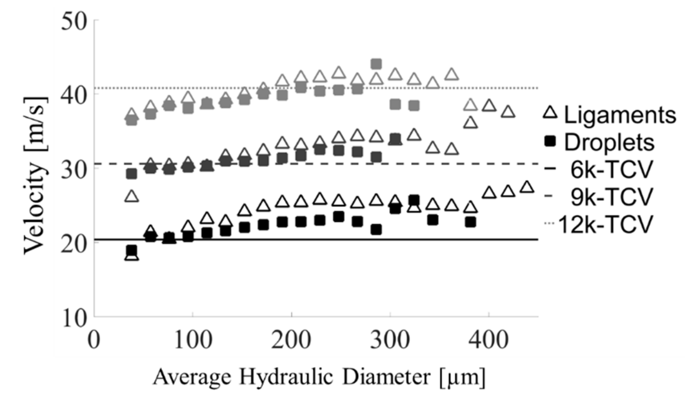
3.3. Velocity Statistics

The fluid velocity distributions for the magnitude of the velocity vectors and both the tangential components of those vectors with respect to the cup are shown in Figure 10. These distributions were calculated in the same manner as the size distributions, but with bin intervals of 2 m/s. Clearly, for each case, as the RPM increases, the velocity magnitude also increases. This result is expected since the bell is rotating at higher rotational speeds, however, the ligaments and droplets peak at different velocities. The vertical lines in Figure 10 indicate the magnitude of the tangential speed for each case. As the bell speed increases, the peak ligament velocity approaches the tangential cup velocity, but is greater than the tangential cup velocity for low RPM. In contrast, the peaks for the droplet distributions are centered approximately at the tangential cup velocity across all cases. An interesting result, however, is the apparent broadening of the tangential velocity distributions to the left of their peaks across all cases as the rotational speed increases in Figure 10. Such a result means that the fluid distributions begin to increasingly favor smaller velocity vectors as rotational speed is increased. This could be indicative of more collisions happening or increased interference from air recirculation, which would result in greater numbers of fluid particles being slowed.

The mean velocity was calculated for both the velocity vectors and the tangential component of the velocity vectors for their respective ligaments-only, droplets-only, and overall data sets. The results of these calculations can be seen in

Table 3. Comparison of the mean velocity values for the original velocity vectors and the tangential component velocity vectors at each bell speed tested to the calculated tangential cup speed.

Measured Quantities	Bell Speed [kRPM]
	5	6	7	8	9	10	11	12
Tangential Cup Speed [m/s]
	17.0	20.4	23.8	27.2	30.6	34.0	37.4	40.8
Vavg—Total [m/s]
Ligaments	20.3	24.9	26.7	28.9	32.9	36.3	38.7	40.9
Droplets	18.5	21.7	24.8	27.3	30.8	32.9	35.6	37.9
Combined	19.0	22.5	25.2	27.6	31.2	33.4	36.0	38.2
Vavg—Tangential [m/s]
Ligaments	16.9	21.5	25.2	27.1	30.0	33.7	36.6	38.5
Droplets	15.6	18.7	21.9	24.5	27.9	29.9	32.8	35.0
Combined	16.0	19.4	22.6	25.0	28.3	30.5	33.3	35.4

, compared to the calculated tangential cup speed, based on the RPM and cup diameter. These calculated values further show that as bell speed is increased, droplet and ligament velocities also increase, as expected.

Additionally, the average tangential component of velocity for the ligaments, across all cases, is almost exactly that of the calculated tangential cup speed. This result makes sense given that the ligaments were defined as fluid elements still attached to the cup, and therefore their velocity should essentially match. Notably, the values show that despite the locations of the peaks of the droplets-only velocity distributions approximating the tangential cup speed, the ligaments-only data is the case that has a mean closest to the tangential cup speed. This implies that the detached droplets are experiencing acceleration or deceleration likely due to the shaping airflow, even at such a close proximity to the cup.

Most of these results are expected, though they have not been explicitly found in the literature. Next, the average velocity conditioned on particle size was computed, as shown in Figure 11, to study the effect of particle size on these velocity vectors. These values were calculated by conditionally averaging the velocities of fluid particles within specified diameter bins. The results again show the expected result that the ligaments are moving faster than the droplets in the flow, independent of size. However, they also demonstrate that the larger fluid particles, both ligaments and droplets, move at higher velocities at larger sizes. Thus, the performance of the combined optical setup and image processing allowed for size and velocity data for all fluid particles in the images, from a single data set. It is worth noting that recent work showed that larger droplets tend to have slower impact velocities closer to target in high speed rotary bells [44]. Further investigation is needed to understand the trend transition in the spray flowfield (plume).

4. Conclusions

Using high-speed shadowgraph imaging, qualitative ligament breakup mechanisms were observed and quantitative droplet and ligament sizes were measured for a rotary bell atomizer, with the inclusion of shaping air, near its cup edge for eight operational bell speeds. In regards to the qualitative observations of the ligament to droplet breakup for the conditions tested, several notable trends were found. First was that there were multiple ligament breakup regimes for a given rotational speed. The first of these regimes was that of a ligament forming an unstable, mushroom-tip as it grows, and then having that fluid mass eject as a droplet while the rest of the ligament forms into satellite droplets along its length. The next two regimes were different forms of bag breakup where a bag of fluid is formed at the end of a ligament and eventually explodes into satellite droplets. As rotational speed was increased, the dominance of the first type of regime also increased. The two bag breakup regimes were also seen to evolve and become more catastrophic in their breakup. Visually, the ligaments in the images can also be seen to become shorter, and breakup faster, with higher rotational speed. Other changes with increasing rotational speed are an increase in ligament angle to the cup and an increase in the number of satellite droplets in a given fluid disintegration. Further investigation into modeling or predicting these ligament structures and behaviors under these conditions is necessary.

The imaging technique used also allowed for a large quantitative sampling of both droplet and ligament sizes. An image post-processing method was utilized to distinguish between the fluid particles and background illumination accounting directly for frame-to-frame variations in background signal. Once the images were binarized, the fluid sizes were calculated. In addition, images of only the droplets, with very little background noise were used to calculate velocity vectors and to correlate these velocities to individual particles.

This method was demonstrated on water as opposed to paint. However, it is easier to image paint using shadowgraph than it is with water for a couple of reasons. First, paint is more opaque and much more viscous than water. Therefore, the droplets have clearer edges in the images, much slower breakup times, and larger sizes, assuming all operational parameters are equal. It can be assumed that the resulting shadowgraph data would also be applicable for the image processing of paint experiments.

The resulting size distributions showed that both ligament and droplet hydraulic diameters, as well as overall ligament length and width, decrease with increased RPM. The distributions also illustrated that ligaments have a bimodal size distribution, indicating two separate regimes of ligament size in the images. The droplets, however, appeared to have a singular mode size distribution with a slight skew towards larger droplets that began to narrow with increasing rotational speed. This result suggests that the range of droplet sizes, in the field of view imaged and within the parameter ranges tested, narrows with increasing RPM.

The post-processed images were examined using PIV and PTV to determine droplet and ligament velocities. The raw velocity magnitude distributions indicate that the droplet velocities center on the tangential cup velocity, while the ligament velocities center near a velocity that is slightly higher than the tangential cup speed, but maintain an average velocity very close to the cup speed. This result could be an artifact of the effect of the liquid flow velocity or shaping airflow in the system. The velocity magnitude distributions show that as cup speed increases, the ligament velocity distribution begins to approach the tangential cup speed. This indicates the peaks are more closely approaching the numerical average of the ligament data and that other forces in the system become less important if bell speed is sufficiently increased at these parameters. These results are also reaffirmed by the hydraulic diameter relation to average velocity that show the same trend for ligament and droplet velocities with respect to the tangential cup speed.

To conclude, an image processing method was developed to gather relevant data from a rotary bell atomization system operating at relevant parameters to that of an assembly plant, all from a single set of image data that was captured continuously. The method demonstrated both that it could produce data that matched results found in the literature, and could provide some new insight into fluid interactions and trends within the rotary bell atomization process. Future application of this tool could be in the monitoring of in-use bell applicators to allow for feedback on potential changes in specified, relevant flow parameters. Such development would be even more relevant to possible paint application in assembly plants.

References

1. Khan, M.K.I.; Schutyser, M.A.I.; Schroën, K.; Boom, R. The potential of electrospraying for hydrophobic film coating on foods. J. Food Eng. 2012, 108, 410–416. [Google Scholar] [CrossRef]
2. Craig, I.P.; Hewitt, A.; Terry, H. Rotary atomiser design requirements for optimum pesticide application efficiency. Crop Prot. 2014, 66, 34–39. [Google Scholar] [CrossRef]
3. Akafuah, N.; Poozesh, S.; Salaimeh, A.; Patrick, G.; Lawler, K.; Saito, K. Evolution of the automotive body coating process—A Review. Coatings 2016, 6, 24. [Google Scholar] [CrossRef]
4. Domnick, J.; Thieme, M. Atomization characteristics of high-speed rotary bell atomizers. At. Sprays 2006, 16, 857–874. [Google Scholar]
5. Poozesh, S.; Akafuah, N.; Saito, K. Effects of automotive paint spray technology on the paint transfer efficiency—A review. Proc. Inst. Mech. Eng. Part D J. Automob. Eng. 2017, 232, 282–301. [Google Scholar] [CrossRef]
6. Im, K.S.; Lai, M.C.; Yi, L.; Sankagiri, N.; Loch, T.; Nivi, H. Visualization and measurement of automotive electrostatic rotary-bell paint spray transfer processes. J. Fluids Eng. 2001, 123, 237–245. [Google Scholar] [CrossRef]
7. Bailey, A.G. Electrostatic atomization of liquids. Sci. Prog. Oxf. 1974, 61, 555–585. [Google Scholar]
8. Balachandran, W.; Bailey, A.G. The dispersion of liquids using centrifugal and electrostatic forces. IEEE Trans. Ind. Appl. 1984, IA-20, 682–686. [Google Scholar] [CrossRef]
9. Frost, A.R. Rotary atomization in the ligament formation mode. J. Agric. Eng. Res. 1981, 26, 63–78. [Google Scholar] [CrossRef]
10. Corbeels, P.L.; Senser, D.W.; Lefebvre, A.H. Atomization characteristics of a highspeed rotary-bell paint applicator. At. Sprays 1992, 2, 87–99. [Google Scholar] [CrossRef]
11. Debler, W.; Yu, D. The break-up of laminar liquid jets. Proc. R. Soc. Lond. A Math. Phys. Sci. 1988, 415, 107–119. [Google Scholar] [CrossRef]
12. Ellwood, K.R.J. Laminar jets of Bingham-plastic liquids. J. Rheol. 1990, 34, 787–812. [Google Scholar] [CrossRef]
13. Marmottant, P.; Villermaux, E. Fragmentaion of stretched liquid ligaments. Phys. Fluids 2004, 16, 2732–2741. [Google Scholar] [CrossRef]
14. Bizjan, B.; Širok, B.; Hočevar, M.; Orbanić, A. Liquid ligament formation dynamics on a spinning wheel. Chem. Eng. Sci. 2014, 119, 187–198. [Google Scholar] [CrossRef]
15. Ahmed, M.; Youssef, M.S. Characteristics of mean droplet size produced by spinning disk atomizers. J. Fluids Eng. 2012, 134, 71103. [Google Scholar] [CrossRef]
16. Peng, H.; Wang, N.; Wang, D.; Ling, X. Experimental study on the critical characteristics of liquid atomization by a spinning disk. Ind. Eng. Chem. Res. 2016, 55, 6175–6185. [Google Scholar] [CrossRef]
17. Bizjan, B.; Širok, B.; Hočevar, M.; Orbanić, A. Ligament-type liquid disintegration by a spinning wheel. Chem. Eng. Sci. 2014, 116, 172–182. [Google Scholar] [CrossRef]
18. Senuma, Y.; Hilborn, J.G. High speed imaging of drop formation from low viscosity liquids and polymer melts in spinning disk atomization. Polym. Eng. Sci. 2002, 42, 969–982. [Google Scholar] [CrossRef]
19. Kim, T.S.; Kim, M.U. The flow and hydrodynamic stability of a liquid film on a rotating disc. Fluid Dyn. Res. 2009, 41, 035504. [Google Scholar] [CrossRef]
20. Ahmed, M.; Youssef, M.S. Influence of spinning cup and disk atomizer configurations on droplet size and velocity characteristics. Chem. Eng. Sci. 2014, 107, 149–157. [Google Scholar] [CrossRef]
21. Huang, H.; Lai, M.-C.; Meredith, W. Simulation of spray transport from rotary cup atomizer using KIVA-3V. In Proceedings of the ICLASS’00, Pasadena, CA, USA, 16–20 July 2000; pp. 1435–1437. [Google Scholar]
22. Dombrowski, N.; Lloyd, T.L. Atomisation of liquids by spinning cups. Chem. Eng. J. 1974, 8, 63–81. [Google Scholar] [CrossRef]
23. Ellwood, K.R.J.; Tardiff, J.L.; Alaie, S.M. A Simplified analysis method for correlating rotary atomizer performance on droplet size and coating appearance. J. Coat. Technol. Res. 2014, 11, 303–309. [Google Scholar] [CrossRef]
24. Blaisot, J.B.; Yon, J. Droplet size and morphology characterization for dense sprays by image processing: Application to the diesel spray. Exp. Fluids 2005, 39, 977–994. [Google Scholar] [CrossRef]
25. MacIan, V.; Payri, R.; Garcia, A.; Bardi, M. Experimental evaluation of the best approach for diesel spray images segmentation. Exp. Tech. 2012, 36, 26–34. [Google Scholar] [CrossRef]
26. Ma, Y.J.; Huang, R.H.; Deng, P.; Huang, S. the development and application of an automatic boundary segmentation methodology to evaluate the vaporizing characteristics of diesel spray under engine-like conditions. Meas. Sci. Technol. 2015, 26, 45004. [Google Scholar] [CrossRef]
27. Cao, Z.M.; Nishino, K.; Mizuno, S.; Torii, K. PIV Measurement of internal structure of diesel fuel spray. Exp. Fluids 2000, 29, S211–S219. [Google Scholar] [CrossRef]
28. Hess, C.F.; L’Esperance, D. Droplet Imaging Velocimeter and Sizer: A Two-dimensional technique to measure droplet size. Exp. Fluids 2009, 47, 171–182. [Google Scholar] [CrossRef]
29. Zhang, M.; Xu, M.; Hung, D.L.S. Simultaneous two-phase flow measurement of spray mixing process by means of high-speed two-color PIV. Meas. Sci. Technol. 2014, 25, 95204. [Google Scholar] [CrossRef]
30. Stevenin, C.; Tomas, S.; Vallet, A.; Amielh, M.; Anselmet, F. Flow characteristics of a large-size pressure-atomized spray using DTV. Int. J. Multiph. Flow 2016, 84, 264–278. [Google Scholar] [CrossRef]
31. Ryan, S.D.; Gerber, A.G.; Holloway, A.G.L.; Brunswick, N. A computational study of sprays produced by rotary cage atomizers. Trans. ASABE 2012, 55, 1133–1148. [Google Scholar] [CrossRef]
32. Soumendra, B.K.; Zhou, J.; Harding, A.; Williams, C.; Moncier, J.; Baker, L.; McCreight, K. Effect of atomization and rheology control additives on particle size and appearance of automotive coatings. In Proceedings of the 15th International Coating Science and Technology Symposium, St. Paul, MN, USA, 13–15 September 2010. [Google Scholar]
33. Goldsworthy, L.C.; Bong, C.; Brandner, P.A. Measurements of diesel spray dynamics and the influence of fuel viscosity using PIV and shadowgraphy. At. Sprays 2011, 21, 167–178. [Google Scholar] [CrossRef]
34. Ogasawara, S.; Daikoku, M.; Shirota, M.; Inamura, T.; Saito, Y.; Yasumura, K.; Shoji, M.; Aoki, H.; Miura, T. Liquid atomization using a rotary bell cup atomizer (influence of flow characteristics of liquid on breakup pattern). J. Fluid Sci. Technol. 2010, 5, 464–474. [Google Scholar] [CrossRef]
35. Hatayama, Y.; Haneda, T.; Shirota, M.; Inamura, T.; Daikoku, M.; Soma, T.; Saito, Y.; Aoki, H. Formation and breakup of ligaments from a high speed rotary bell cup atomizer (Part 1: Observation and quantitative evaluation of formation and breakup of ligaments). Trans. Jpn. Soc. Mech. Eng. Ser. B 2013, 79, 1081–1094. [Google Scholar] [CrossRef]
36. Majithia, A.K.; Hall, S.; Harper, L.; Bowen, P.J. Droplet breakup quantification and processes in constant and pulsed air flows. In Proceedings of the European Conference on Liquid Atomization and Spray Systems, Como Lake, Italy, 8–10 September 2008; pp. 8–10. [Google Scholar]
37. Stevenin, C.; Béreaux, Y.; Charmeau, J.-Y.; Balcaen, J. Shaping air flow characteristics of a high-speed rotary-bell sprayer for automotive painting processes. J. Fluids Eng. 2015, 137, 111304. [Google Scholar] [CrossRef]
38. Domnick, J.; Scheibe, A.; Ye, Q. The simulation of electrostatic spray painting process with high-speed rotary bell atomizers. Part II: External charging. Part. Part. Syst. Charact. 2006, 23, 408–416. [Google Scholar] [CrossRef]
39. Gonzalez, R.C.; Woods, R.E. Digital Image Processing, 2nd ed.; Prentice Hall: Englewood Cliffs, NJ, USA, 2002. [Google Scholar]
40. Rao, D.C.K.; Karmakar, S.; Basu, S. Atomization characteristics and instabilities in the combustion of multi-component fuel droplets with high volatility differential. Sci. Rep. 2017, 7, 8925. [Google Scholar] [CrossRef] [PubMed]
41. Jain, M.; Prakash, R.S.; Tomar, G.; Ravikrishna, R.V. Secondary breakup of a drop at moderate weber numbers. Proc. R. Soc. A Math. Phys. Eng. Sci. 2015, 471, 20140930. [Google Scholar] [CrossRef]
42. Zhao, H.; Liu, H.F.; Li, W.F.; Xu, J.L. Morphological classification of low viscosity drop bag breakup in a continuous air jet stream. Phys. Fluids 2010, 22, 114103. [Google Scholar] [CrossRef]
43. Cao, X.K.; Sun, Z.G.; Li, W.F.; Liu, H.F.; Yu, Z.H. A new breakup regime of liquid drops identified in a continuous and uniform air jet flow. Phys. Fluids 2007, 19, 057103. [Google Scholar] [CrossRef]
44. Ye, Q.; Domnick, J. Analysis of droplet impingement of different atomizers used in spray coating processes. J. Coat. Technol. Res. 2017, 14, 467–476. [Google Scholar] [CrossRef]
Figure 1. Experimental diagram with lamp (A), rotary bell (B), camera (C), hood (D) and computer (E). Also pictured are the rotary bell (F) and an experimental image (G) with direction of cup rotation (left arrow) and the general fluid flow direction (right arrow) indicated.
Coatings 08 00174 g001
Figure 2. Image processing steps visualization, which includes the original image (a); dilated image (b); subtraction (c); binarization (d); ligaments-only image (e); droplets-only image (f); and edges of binarization imposed on the original image (g).
Coatings 08 00174 g002
Figure 3. Number distributions of ligament size for the 6000 RPM case after the inclusion of the data from varying amounts of frames, n.
Coatings 08 00174 g003
Figure 4. Convergence of percent difference compared to the inclusion the entire data set, of the number distributions of ligament size by including varying amounts of frames for three different bell speeds.
Coatings 08 00174 g004
Figure 5. Image sequences of three different ligaments in the 5 kRPM case over time (moving from left to right in the respective row): elongated ligament into droplet (a); ligament into bag breakup (b); and bag breakup off of the cup (c). These images within each sequence were taken 15 frames, or 44.1 μs, apart. The boxed liquid structure is the liquid of interest.
Coatings 08 00174 g005
Figure 6. Image sequences of three different ligaments in the 8 kRPM case over time (moving from left to right in the respective row): elongated ligament into droplet (a); ligament into bag breakup (b); and bag breakup off of the cup (c). These images within each sequence were taken 10 frames, or 29.4 μs, apart. The boxed liquid structure is the liquid of interest.
Coatings 08 00174 g006
Figure 7. Image sequences of three different ligaments in the 12 kRPM case over time (moving from left to right in the respective row): elongated ligament into droplet (a); ligament into bag breakup (b); and bag breakup off of the cup (c). These images within each sequence were taken 7 frames, or 20.6 μs, apart. The liquid structure of interest is boxed for convenience.
Coatings 08 00174 g007
Figure 8. Number (ac) and volumetric (df) distributions of droplets (b,e), ligaments (c,f) and both (a,d) for the 6000 RPM, 9000 RPM, and 12,000 RPM bell speed cases in 20 μm intervals and then normalizing the curves by the sum of the distribution.
Coatings 08 00174 g008
Figure 9. Ligament length (a) and width (b) number distributions for the 6000 RPM, 9000 RPM and 12,000 RPM bell speed cases.
Coatings 08 00174 g009
Figure 10. Velocity number distributions of ligaments (c,f), droplets (b,e) and both (a,d), and associated tangential cup velocity (TCV) plotted as vertical lines for the 6000 RPM, 9000 RPM, and 12,000 RPM bell speed cases.
Coatings 08 00174 g010
Figure 11. Velocity vs. size distributions of ligaments (triangles) and droplets (squares) and the associated tangential cup velocity (horizontal lines) for the 6000 RPM (solid), 9000 RPM (dashed) and 12,000 RPM (dotted) tangential cup velocities.
Coatings 08 00174 g011