
The Thermal Conductivities of Periodic Fibrous Composites as Defined by a Mathematical Model


School of Applied Mathematics and Physical Sciences NTUA, Section of Mechanics, 5 Heroes of Polytechnion Avenue, GR-15773 Athens, Greece
*
Author to whom correspondence should be addressed.
Fibers 2017, 5(3), 30; https://doi.org/10.3390/fib5030030
Submission received: 4 May 2017
/
Revised: 1 August 2017
/
Accepted: 4 August 2017
/
Published: 14 August 2017
(This article belongs to the Special Issue Fiber Reinforced Polymer Composites or Polymer-Carbon Nanotube Nanocomposites)
Abstract
:In this paper, a geometric body-centered model to simulate the periodic structure of unidirectional fibrous composites is presented. To this end, three prescribed configurations are introduced to predict in a deterministic manner the arrangement of internal and neighboring fibers inside the matrix. Thus, three different representative volume elements (RVEs) are established. Furthermore, the concept of the interphase has been taken into account, stating that each individual fiber is encircled by a thin layer of variable thermomechanical properties. Next, these three unit cells are transformed in a unified manner to a coaxial multilayer cylinder model. This advanced model includes the influence of fiber contiguity in parallel with the interphase concept on the thermomechanical properties of the overall material. Then, by the use of this model, the authors propose explicit expressions to evaluate the longitudinal and transverse thermal conductivity of this type of composite. The theoretical predictions were compared with experimental results, as well as with theoretical values yielded by some reliable formulae derived from other workers, and a reasonable agreement was found.
1. Introduction
To predict the rheological and thermomechanical behavior of unidirectional fibrous composites, many influential factors can be taken into consideration. Roughly speaking, these parameters are able to be grouped in the following three categories: those depending on the arrangement and orientation of fibers, those depending on the type of matrix, which mostly is polymeric, and finally, those depending on the fiber matrix interaction or adhesion. Actually, fiber reinforcement makes the composite much stronger when compared with a pure polymer. Yet, a disadvantage of uniaxial fibrous composites is that the fibers can transmit loads only in the direction of their axis, and unfortunately, there is less of a strengthening effect in the direction perpendicular to the axis.
On the other hand, the role of the matrix is mainly to protect the fiber from the corrosive action of the environment and also to ensure interactions amongst the fibers by mechanical, physical and chemical effects. In the fibrous reinforced composites, the deformation of the matrix evidently transfers stresses to the embedded high-strength fibers by means of shear tractions at the fiber matrix interface. Meanwhile, fibers retard the propagation of cracks and thus produce a material of high strength. To simulate the microstructure of such materials, a large number of microstructural models appeared in the literature.
Rayleigh’s method [1] leads to analytical expressions for longitudinal and transverse thermal conductivities of fibrous composites where a continuous matrix is reinforced with parallel cylindrical fibers arranged in a uniaxial simple cubic array. Yet, for high filler contents, the results are not realistic [1].
Hashin and Rosen’s cylinder assemblage model [2,3] constitutes a basic and confident approach for the microstructural simulation of two-phase unidirectional fibrous materials, whereas Springer and Tsai [4] introduced a shear loading analogy approach in order to calculate the longitudinal and transverse thermal conductivities of fibrous composites.
Nonetheless, there are several models that take into account the existence of an intermediate natural phase, developed during the preparation of the composite material and which plays an important role in the overall thermomechanical behavior of the composite.
In [5,6] the previously mentioned third phase (interphase) was assumed as a homogeneous and isotropic, whereas in [7], an improved model was suggested, according to which the fiber was surrounded by a series of successive cylinders, each of which has a different elastic modulus in a step-function variation with the polar radius.
Moreover, mathematical analyses of inhomogeneous natural interphase zones started, probably, with the work of Kanaun and Kudryavtseva [8] on the effective elasticity of a medium with spherical inclusions encircled by radially-inhomogeneous interphase zones. In this remarkable work, the fundamental concept of replacing an inhomogeneous inclusion by an equivalent homogeneous one was advanced. Such a replacement was carried out by modeling the inhomogeneous interface by a number of thin concentric layers (piecewise constant variation of properties). An analogous analysis for cylindrical inhomogeneities (fibers) surrounded by concentric layers was carried out by the same authors [9].
In addition, a valuable experimental investigation towards the estimation of mechanical and thermal properties of fibrous composite materials was carried out by Clements and Moore [10]. In the past years, a lot of recent research work has been carried out for the determination of thermomechanical properties of unidirectional fibrous composite materials and for the investigation of the influence of the aforementioned important parameters, i.e., filler-matrix interaction, adhesion efficiency, fiber arrangement and vicinity, etc.
Caruso et al. [11] and Muralidhar [12] addressed valuable theoretical approaches for predicting the thermal conductivities of fibrous composite materials. Furthermore, in [13], the influence of fiber packing on the elastic properties of a transversely-random unidirectional glass/epoxy composite was investigated, whilst Huang [14] gave a micromechanical prediction of the ultimate strength of transversely isotropic fibrous composite materials.
On the other hand, for a detailed experimental study on the thermal conductivities of fiber-reinforced composites, measured in three directions (transverse, longitudinal and through the thickness), one may refer to [15].
Furthermore, in [16], a micro-scale simulation and prediction of the mechanical properties of fibrous composites by means of the bridging micromechanics model was carried out, whereas for a thorough study on the effective properties of fibrous composite media of a periodic structure, one may refer to [17].
Besides, an elasticity approach towards the evaluation of the transverse modulus of unidirectional fibrous composites, with the concurrent consideration of an irregular distribution of fibers, was made in [18], while Shah et al. [19] proposed a detailed analysis on the compressive properties of fibrous composites of a polymeric matrix via combined end and shear loading.
In [20], the effective elastic constants for periodic fibrous composites with imperfect contact conditions between fibers and matrix were estimated. The approach adopted to simulate the fiber distribution is a somewhat parallelogram configuration, whilst the imperfectness of the contact is modeled by linear springs. Furthermore, in [21], the concept of the interphase was taken into account to calculate the elastic constants of unidirectional fibrous composites by means of a classical elasticity approach.
In [22], the influence of the statistical character of fiber strength on the predictability of the tensile properties of polymer composites reinforced with natural filler was examined by comparing the well-known linear and power-law Weibull models, whereas in [23], the thermal conductivities of a general class of unidirectional fibrous composites were estimated by the aid of the interphase concept.
Further, in [24], numerical calculations of the effective thermal conductivity of unidirectional fibrous composite materials with an interfacial thermal resistance between the continuous and dispersed components were carried out.
Meanwhile, in [25], a hexaphase coaxial spherical model was introduced to evaluate the thermal conductivity of macroscopically homogeneous particulate composite materials. This model, obtained from a body-centered cubic model after a topological transformation based on the equality between phase contents, took into account the particle vicinity. Nevertheless, in this model, the concept of the interphase was neglected.
Finally, in [26], the thermal conductivity of particulate composites of a periodic structure was estimated by means of a similar geometric model. This model took into consideration the particle distribution and contiguity together with the concept of the interphase.
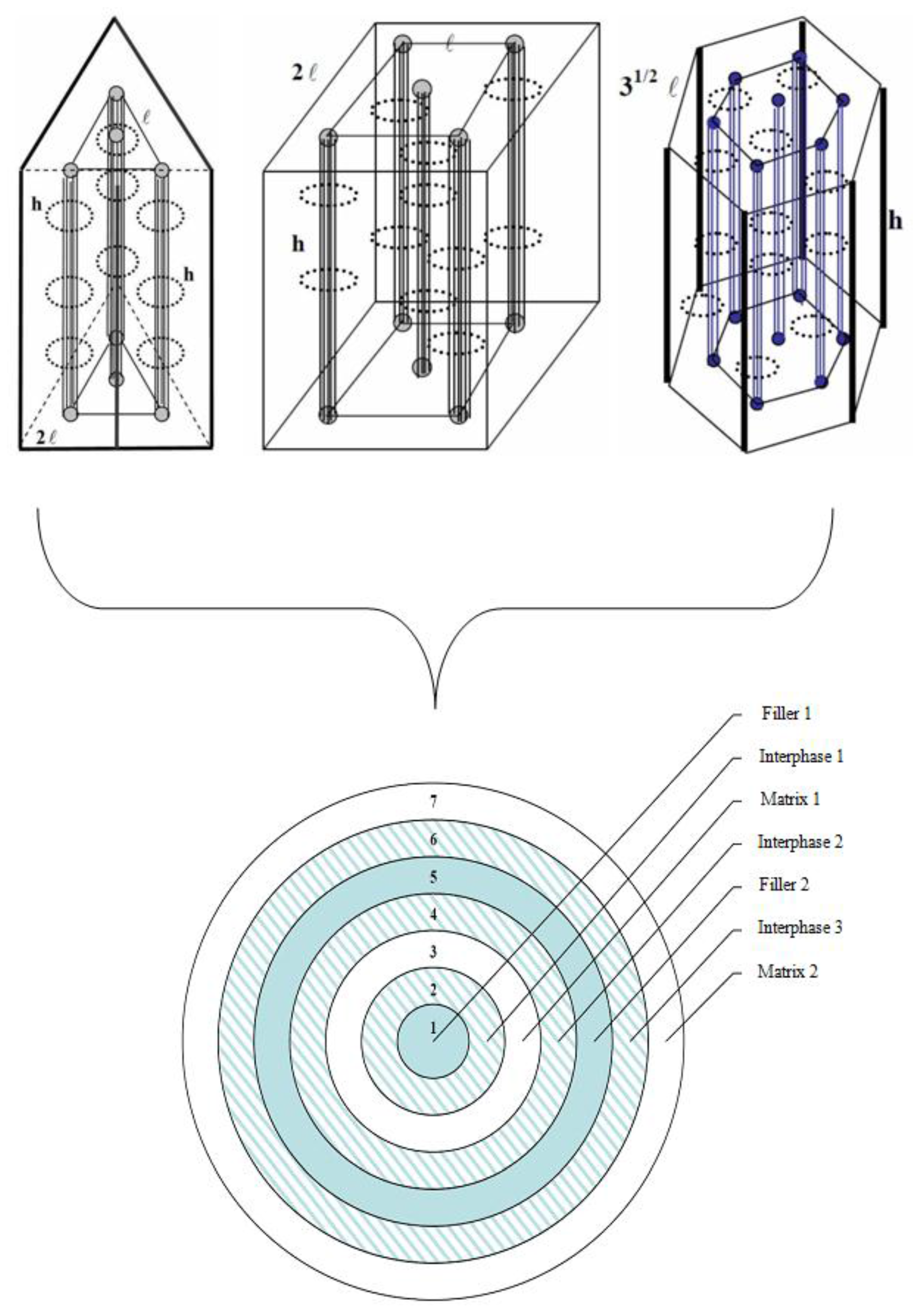
In the present work, the thermal conductivities of periodic fibrous composites are evaluated by means of three prismatic geometric body-centered models, the unit cells of which have been transformed in a unified manner to a seven-phase cylindrical model. This topological transformation is based on the equality between the volume fractions of each separate phase of the prismatic and cylindrical model.
Hence, via this advanced multilayer model, the contiguity amongst the fibers (internal and neighboring), in the form of their deterministic configurations, is examined in parallel with the interphase concept, to calculate the properties of the overall material.
In this context, the authors propose amended forms of the standard and inverse law of mixtures, in order to determine the longitudinal and transverse thermal conductivity of the overall material.
2. Simulation of Fiber Arrangement
As is known, the majority of microstructural models that may concern either particulate or fiber composites aim at the reproduction of the basic cell, or representative volume element (RVE), of the periodic composite at a macroscopic scale in order to obtain a solution. In the case of unidirectional fibrous composites, the following simplified assumptions are generally adopted:
- (i)
- The fibers are perfectly cylindrical in shape.
- (ii)
- All cross-sectional areas of the cylindrical model have the same microstructure.
- (iii)
- The matrix and the fibers are elastic, isotropic and homogenous, and the fiber arrangement is uniform so that no agglomeration occurs.
In this investigation, we shall attempt to predict the fiber distribution inside the matrix introducing three geometric models.
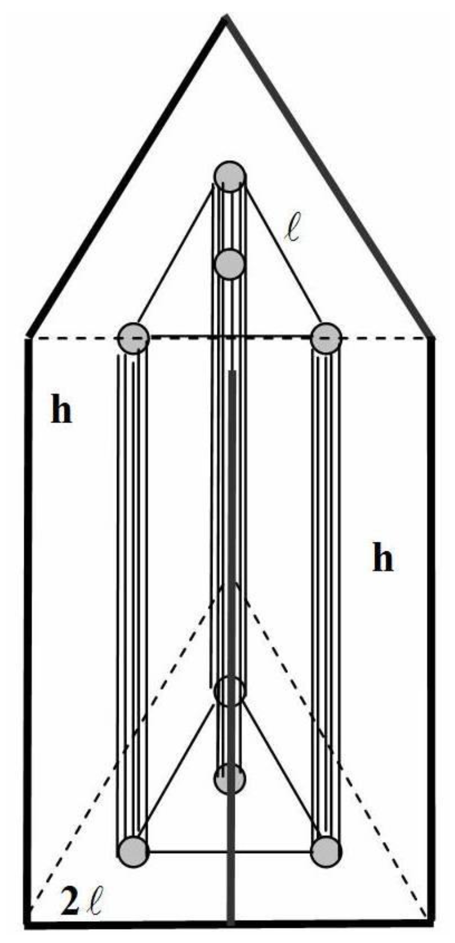
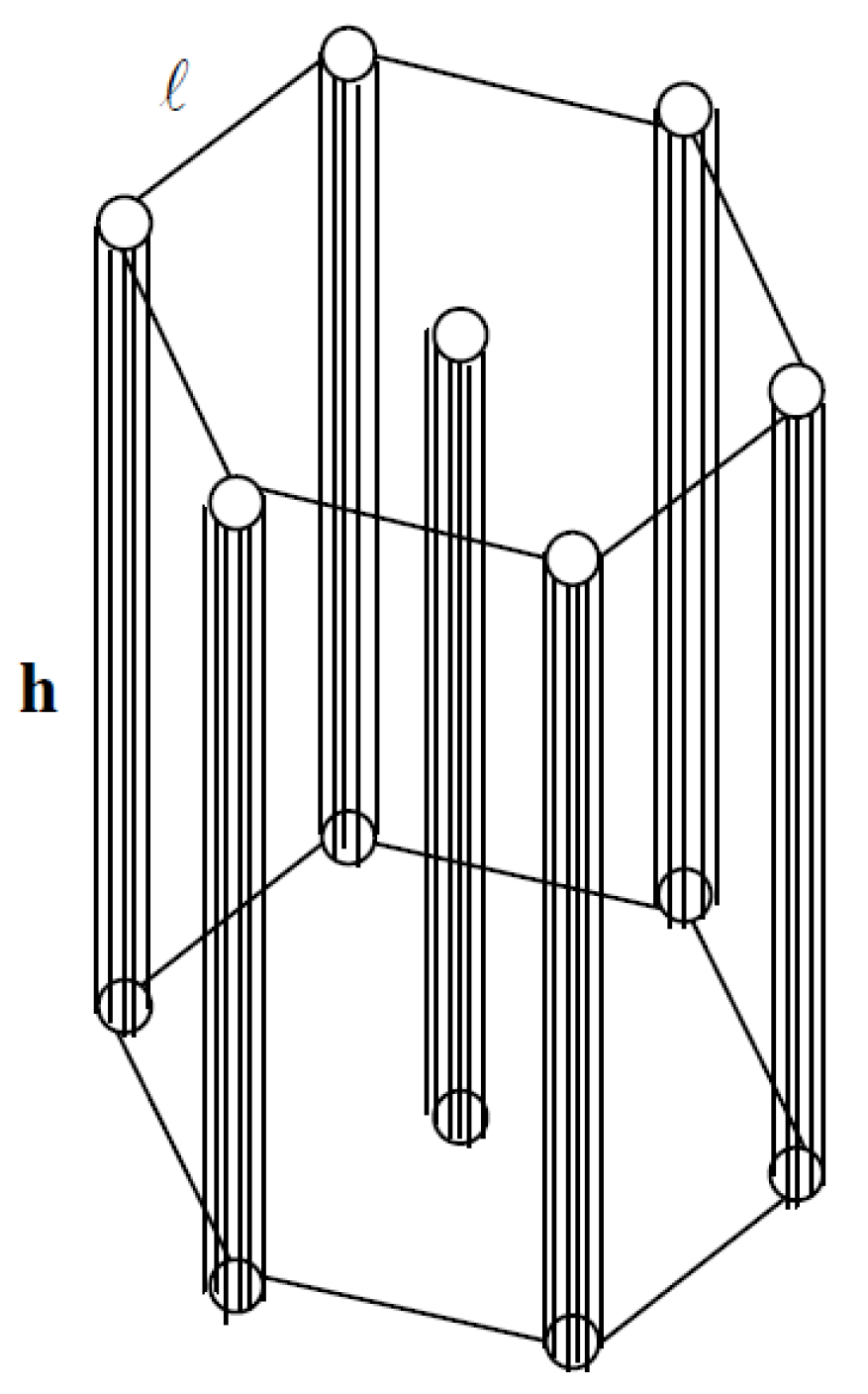
Let us initiate our analysis presenting a triangular prismatic body-centered model of rectangular sides appearing in Figure 1.
Here, one may point out that the fibers occupy the vertices and the centroid axis of a triangular prism of edge and height h. Next, to create a unit cell capable of simulating unidirectional fibrous composites of a periodic structure, one may consider a second prism of side so as to circumscribe the first one, as can be seen in Figure 2.
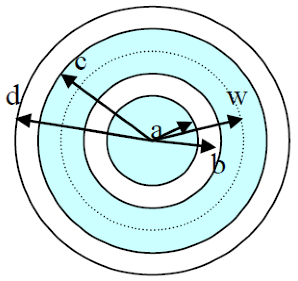
The above unit cell is reproduced in space in a symmetrical manner, and therefore, it can describe a periodic, unidirectional fibrous composite of ideal fibers. Then, to facilitate our investigation, we may transform the above microstructural model into a four-phase cylindrical model consisting of four concentric cylinders of the radii a, b, c, d, respectively, such that a < b < c < d. The cross-sectional area of this model is illustrated in Figure 3.
As has been already elucidated, the above topological transformation is based on the equality between the contents of each separate phase of the prismatic and cylindrical unit cells.
Evidently, the second and fourth phase (the cylindrical region of inner radius a, and outer radius b and the cylindrical region of inner radius c and outer radius d) represent the matrix.
Furthermore, the central cylinder of radius a, i.e., the first phase, together with the cylindrical region of inner radius b and the outer one c, i.e., the third phase, represent the fibers.
Here, one may emphasize that the blank matrix phase that surrounds the external fibers in the prismatic unit cell, or equivalently the second fiber zone in the coaxial cylindrical model, warrants that no agglomeration will appear.
On the other hand, it is known from Euclidean geometry that the volume V of a triangular prism of edge is given as:
Besides, the fiber volume fraction Uf is estimated as:
and therefore:
According to our proposed geometric transformation, the volume of a triangular prism of edge reduces to the volume of a cylinder of radius d. Hence, one infers:
Furthermore, since it is evident that the first phase of the cylindrical model (Figure 3) encircles the centroid axis of the triangular prism, it follows:
Moreover, in the prismatic model of Figure 1, let be the distance between the centroid axis and each vertex.
Hence, the following relationship holds:
Here, without violating our proposed formalism, let us also assume that in the four-phase model occurring in Figure 3, the circle of radius , drawn by dotted line, lies in the middle of the circular section, which denotes the third phase.
Thus, the following relationships arise:
and:
Solving the above system for b and c, respectively, one obtains:
Moreover, the following geometric restrictions hold:
The first restriction yields:
Furthermore, according to the second constraint, it follows:
Hence, the performed prismatic model transformed into a four-phase cylindrical model can be valid when Uf 92.25%.
In continuing, let us consider the following square body-centered prismatic model (Figure 4).
Following the same reasoning as before, let us design the RVE below, which obviously is able to simulate unidirectional fibrous composites of a periodic structure (Figure 5).
Next, to simplify the analysis, utilizing the structural symmetries of the above model, we may transform it into the same four-phase cylindrical model, the cross-section of which first appeared in Figure 3.
Meanwhile, the volume V of a square prism of edge is given as:
Furthermore, in this model, the fiber content is evaluated as:
and therefore:
Taking into account the proposed topological transformation, the volume of a square right prism of edge reduces again to the volume of a cylinder of radius d. Hence, we infer:
Equation (16) can be combined with Equation (15) to yield:
In addition, it is obvious that the first phase of the cylindrical model (Figure 3) should surround the centroid axis of the square prism, and therefore, the validity of Equation (5) also concerns the second prismatic model.
Now, in the square prism of Figure 4, the distance between the centroid axis and each vertex is given as:
Moreover, since we have already considered that in the four-phase model occurring in Figure 3, the circle of radius lies in the middle of the circular section denoting the third phase, Equation (7) still holds, whereas Equation (8) is replaced by:
Solving the system of Equations (7) and (18) for b and c, respectively, one obtains:
Moreover, the geometric constraints expressed by Inequality (10) are valid for this model, as well.
Now, the first restriction yields:
Furthermore, according to the second restriction, one infers:
Thus, the second prismatic model is valid for Uf 74.99%.
Finally, let us present the following hexagonal prismatic microstructural model (Figure 6). The corresponding unit cell of this model appears just below (Figure 7).
Then, to accommodate our analysis, taking also into account the evident structural symmetries of the above hexagonal prismatic model, we may transform it again into the same four-phase cylindrical model of Figure 3.
On the other hand, the volume of a hexagonal prism of edge is given as:
Concurrently, the filler content is calculated as:
and therefore:
Taking into consideration the performed geometric transformation, the volume of a hexagonal prism of edge reduces to the volume of a cylinder of radius d.
Hence, we deduce that:
Hence, the latter equation combined with (25) yields:
Evidently, the first phase of the cylindrical model of Figure 3 should encircle the centroid axis of the hexagonal prism, and therefore, we deduce that the validity of Equation (5) concerns the third model, as well.
Besides, in the hexagonal prismatic model of Figure 6, the distance between the centroid axis and each vertex is given as:
In addition, since we have supposed beforehand that in the four-phase model of Figure 3, the circle with radius lies in the middle of the circular section denoting the third phase, it implies that Equation (7) still holds, whereas Equation (8), is now replaced by the following relationship.
The solution of the system of Equations (7) and (30) for b, c, respectively, yields:
Meanwhile, the geometric restrictions arising from Equation (10) are also valid for this model.
Here, the first constraint yields:
Furthermore, according to the second restriction, one finds:
Consequently, it can be said that the third prismatic model is valid for Uf 84.91%.
3. The Concept of the Interphase: Towards a Seven-Phase Cylindrical Model
The reasons for taking into consideration the concept of the interphase in composite materials, as well as the proof that the introduction of this inhomogeneous phase yields results that are closer to real characteristic values of this type of material have been well established in [27]. In the present investigation, the concept of the interphase will be taken into account along with the fiber arrangement and contiguity on the thermal properties of the entire material. Hence, according to the proposed mathematical formalism, this intermediate natural phase is developed in the form of cylindrical layers of variable properties that surround the internal and neighboring fibers of the previously proposed three right prismatic models, and thus, it adds three more separate phases to the corresponding four-phase coaxial cylindrical model. In this context, the final inhomogeneous cylindrical model according to which we shall estimate the thermal conductivities of the unidirectional fibrous composite material will have seven distinguished phases, as is illustrated in Figure 8.
In this inhomogeneous coaxial multiphase model, the first phase from inside to outside having radius r1 represents the first area of the filler. The second phase is the cylindrical shell with the inner radius r1 and outer radius r2 and represents the first region of the intermediate phase. Furthermore, the third phase is the cylindrical shell of inner radius r2 and outer radius r3 and shows the first region of the matrix. The fourth phase is the cylindrical shell with the inner radius r3 and the outer radius r4 and represents the second region of the intermediate phase. The fifth phase is the cylindrical shell of inner radius r4 and outer radius r5 and represents the second region of the filler. The sixth stage is the cylindrical shell of inner radius r5 and outer radius r6 representing the third region of the interphase. The seventh and last phase is the cylindrical shell with an inner radius r6 and an outer radius r7 and represents the second region of the matrix.
In continuing, we should determine the radii of the three interphases , , along with the interphase volume fractions in the three regions separately. To this end, let us adopt the following notations:
Evidently, the following relationships hold:
Moreover, given that the interphase is considered as somewhat an altered matrix and its proportion is constant wherever it can be developed, we infer:
where:
Furthermore, without violating the generality, let us assume that:
Thus, we obtain:
whereas:
and:
Here, we should emphasize that since the interphase is an altered matrix and thus there is no addition of other materials in our final model, the radii a, b, c, d of the four-phase model introduced in the previous section also appear in the proposed seven-phase model and now have just been renamed as , respectively. Hence, in the above relations, we have expressed the interphase radii of the seven-phase cylindrical model in terms of the radii b, c, d of the four-phase one, which does not contain any intermediate phase. Moreover, the outer radius of the four-phase model remains as is, after the development of the intermediate phase around the fiber. Furthermore, the outer and inner radius of the filler phase in the four-phase model remains the same in the seven-phase model. These results are attributed to the fact that the intermediate phase does not affect the volume in the filler content, only the volume in the matrix content.
According to this viewpoint, we should also emphasize that all restrictions for filler content Uf arising from the geometric constraints of the prismatic models introduced in the previous section, i.e., Inequalities (11), (12), (22), (23), also concern the new seven-phase model. In the sequel, one may evaluate the volume fractions of all phases in terms of the corresponding radii as follows.
On the other hand, the fibrous composite material in reality consists of three different phases (matrix, fiber and interphase) and according to our model is divided into seven distinguished phases.
Lipatov [28] proved that, if calorimetric measurements are performed in the neighborhood of the glass transition zone of the composite, energy jumps are observed. These jumps are too sensitive to the amount of filler added to the matrix and can be used to evaluate the boundary layers developed around the filler. Apparently, as the filler volume fraction is increased, the proportion of macromolecules characterized by a reduced mobility is also increased. This is equivalent to an augmentation of the interphase content and supports the empirical conclusion presented in [28] that the extent of the interphase expressed by its thickness is the cause of the variation of the amplitudes of heat capacity jumps appearing at the glass transition zones of the matrix material and the composite with various filler-volume fractions. Moreover, the size of heat capacity jumps for unfilled and filled materials is directly related to by an empirical relationship given in [28]. This expression defines the interphase thickness and is given as:
In addition, the interphase volume fraction arises from the following expression:
with:
Here, the numerator and the denominator of the fraction appearing in the right member of Equation (32) are the sudden changes of the heat capacity for the filled and unfilled polymer, respectively.
Furthermore, according to the proposed multiphase model, it is evident that:
Concurrently, it has been shown [27,29] that for the unidirectional fiber composites, the following parabolic relationship between the content of the intermediate phase and the filler content holds:
with C defined from the experimental evidence as C = 0.123 [27,29].
Thus, for any ordered couple (, ), by the use of Equation (35) along with Equations (36)–(45), one may calculate the radii of the seven-phase model, provided that the diameter of the cylindrical fibers is known.
4. Materials and Experimental Work
The unidirectional glass-fiber composites used in the experimental part of our investigation consisted of an epoxy matrix (Permaglass XE5/1, Permali Ltd., Bristol, U.K.) reinforced with long E-glass fibers. The matrix material was based on a diglycidyl ether of bisphenol A together with an aromatic amine hardener (Araldite MY 750/HT972, Ciba-Geigy, Bristol, U.K.). The glass fibers had a diameter of 1.2 × 10⁻⁵ m and were contained at a volume fraction of about 65%. The fiber content was determined, as customary, by igniting samples of the composite and weighing the residue, which gave the weight fraction of glass as: Wf = 79.6 ± 0.28%. This and the measured values of the relative densities of Permaglass (pf = 2.55 g/cm3) and of the epoxy matrix (pm = 1.20 g/cm3) gave the value Uf = 0.65. Furthermore, chip specimens with a 0.004-m diameter and thicknesses varying between 0.001 m and 0.0015 m made either of the fiber composite of different filler contents or of the matrix material were tested by the authors on a differential scanning calorimetry (DSC) thermal analyzer at the zone of the glass transition temperature for each mixture, in order to determine the specific heat capacity values.
Moreover, since the samples are discs of 4 mm in diameter and 1 mm in thickness, this implies that their mass is about 50 mg. Furthermore, the thermal conductivity of each fiber is Kf = 1.2 W/m·K, whilst the thermal conductivity of the matrix is Kf = 0.2 W/m·K.
Consequently, the results emerging from the proposed mathematical analysis along with the experimental data are summarized in Table 1, whereas Figure 9 illustrates the variation of the overall interphase content of the composite versus the fiber volume fraction.
Next, in Table 2, we present the concentrated values of volume fractions for the seven phases with respect to filler content. Here, we elucidate that the geometrical constraints found in the previous section were taken into account.
5. Estimation of Thermal Conductivities
As we have emphasized, the concept of the interphase has been considered together with the influence of fiber contiguity on the thermomechanical properties of the composite.
Generally, the coefficient of thermal conductivity of this intermediate phase can be expressed as an n-degree polynomial with respect to the radius r.
To cover the whole spectrum of variation of the quantity , let us suppose five different approaches:
(a) Linear variation:
The first approach is a linear variation of the thermal conductivity of the interphase with respect to radius .
where A and B are quantities varying with respect to the radii of matrix and fiber.
To evaluate these terms, we should take into consideration the following boundary conditions.
At .
Here, we have assumed that the coefficient of thermal conductivity of the interphase, at the boundary with the matrix, coincides with the quantity .
Besides, at the interface between first interphase and filler, the quantity constitutes actually a portion of , which implies that Ki < Kf.
This influence is described by the indicator η, the rates of which belong to the interval . Hence, the following relationship arises.
(b) Parabolic variation
Next, let us assume a parabolic variation of thermal conductivity with respect to the radius .
Hence, the following equality holds:
To estimate the terms A, B and C, which depend on the radii, as well as the thermal conductivities of constituents of the composite, we can also apply the previous boundary conditions.
In addition, one may suppose that all of the parabolas that represent graphically this aforementioned variation should have global minima at the critical values ri. The corresponding mathematical expression of this requirement can be formulated as follows:
Therefore, after the necessary algebraic manipulation, the following relationship arises:
(c) Hyperbolic variation:
In continuation, we assume a hyperbolic variation for Ki(r) as expressed by the following formula:
when .
To calculate the quantities A and B, we may use the same boundary conditions. Thus, it follows:
(d) Logarithmic variation:
According to a logarithmic variation, the term Ki(r) emerges from the following expression:
By taking into account the same boundary conditions as previously, we obtain:
(e) Exponential variation:
Finally, let us suppose that the quantity Ki(r) varies according to a generic exponential law in the following form.
An application of the same boundary conditions as previously yields.
Suggestively, let us select the parabolic variation law with the concurrent consideration that the influence of the interphase becomes maximum, which implies that the coefficient equals unity.
In this context, Equation (53) yields:
Next, to facilitate our derivations, let us estimate the average values of interphase thermal conductivity by the following relationship:
Then, the coefficient of longitudinal thermal conductivity, according to a modified form of the standard law of mixtures, which arises from our proposed multiphase model, is given as:
where denote the thermal conductivities of the composite, filler and matrix, respectively.
In continuing, according to a modified form of the inverse law of mixtures, which also emerges with the aid of the same model, one obtains the following relationship for the transverse thermal conductivity .
Solving Equation (64) for , we obtain:
6. Discussion
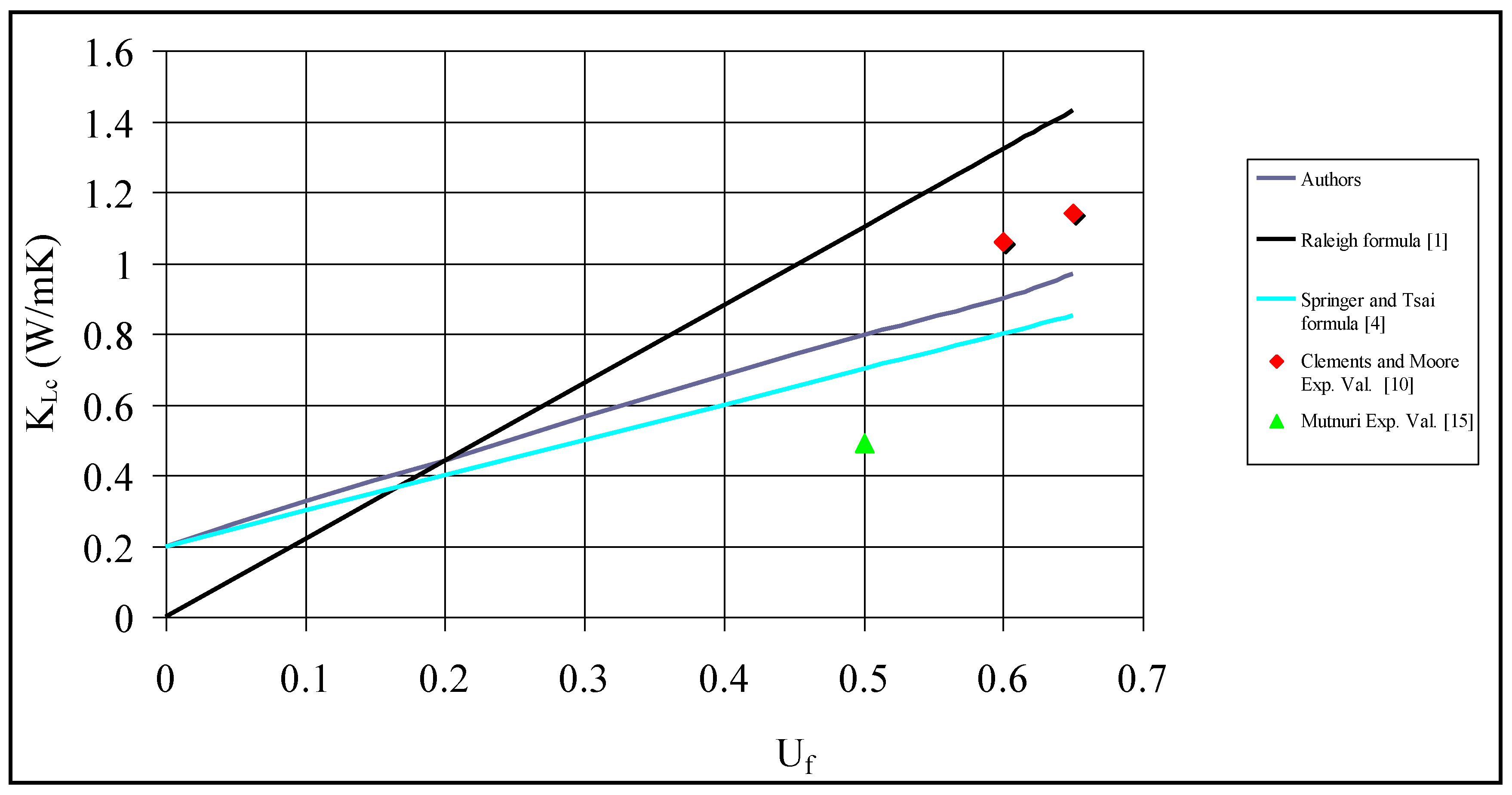
Table 3 presents the average values of interphase thermal conductivity with respect to fiber content as obtained from Equation (62), i.e., according to the parabolic variation law. Besides, the theoretical values of the longitudinal thermal conductivity of the composite yielded by Equation (63) appear along with those arising from two other theoretical formulae derived from Rayleigh [2] and Springer and Tsai [4].
In continuation, Figure 10 illustrates the variation of with respect to fiber volume fraction according to three different theoretical approaches. Here, one may observe that the proposed theoretical formula represented by Equation (63) definitely constitutes an improvement when compared with the classical expression introduced by Springer and Tsai [4]. Moreover, for low fiber contents, the theoretical values obtained from Rayleigh’s formula are below those arising from Equation (63). Yet, for medium filler contents, the values yielded by Rayleigh’s formula surpass those obtained from Equation (63) and for high fiber contents are well above. Nevertheless, it is the authors’ opinion that the occurrence of this discrepancy does not constitute a shortcoming of the introduced formula for longitudinal thermal conductivity, since it has been stated in [1] that the values arising from Rayleigh’s formula for the axis parallel to the fibers are far from reality for high filler contents.
On the other hand, the theoretical predictions for are relatively close to the experimental results for high fiber contents, obtained from Clements and Moore [10], whilst there is a considerable discrepancy of the theoretical values when compared with experimental results for medium fiber contents presented in [15].
However, such discrepancies may be expected because in general, many of the theoretical assumptions and conceptions that concern the microstructural modeling of periodic unidirectional fibrous composite materials cannot be fulfilled in praxis.
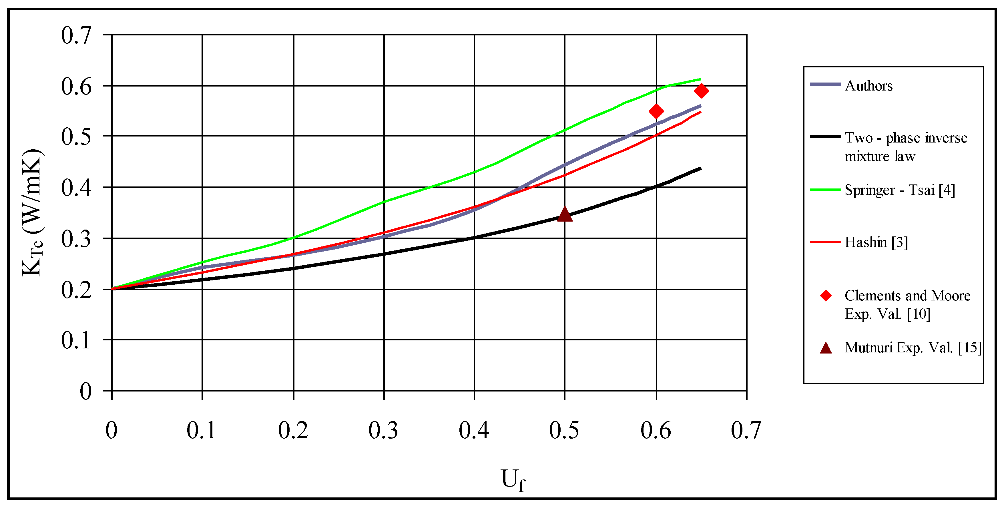
Next, in Table 4, the theoretical values of the transverse thermal conductivity of the composite obtained from Equation (65) occur together with those arising from three accurate theoretical formulae derived from Hashin [2], Springer and Tsai [4] and the inverse rule of mixtures for a two-phase fibrous composite system.
Figure 11 shows the variation of transverse thermal conductivity with respect to filler content according to four theoretical models. Here, one may observe that the values obtained from Springer and Tsai’s formula [4] are well above those arising from Hashin’s formula [3], the two-phase inverse mixture law and finally Equation (65). However, Springer and Tsai’s approach has supposed matrix and fiber as parallel and series as in electrical circuits. Hence, it constitutes a different viewpoint when compared with periodic microstructural models.
Moreover, one may point out that Equation (65) indeed constitutes an improved version of two-phase inverse mixtures law. Besides, the theoretical values yielded by Equation (65) are very close to those arising from Hashin’s fundamental formula for transverse thermal conductivity [3], as well as to experimental results for high volume fractions of fiber reinforcing performed in [10]. Furthermore, the experimental value for medium fiber content (Uf = 0.5) obtained from Mutnuri [15] almost coincides with the corresponding theoretical value yielded by the two-phase inverse mixtures law, whereas it is well below the graphs of Equation (65), the Hashin and Springer-Tsai formulae with respect to Uf.
For a brief description of the theoretical formulae selected for comparison, one may see the Appendix.
Here, one may elucidate that in the previously presented analysis towards the estimation of thermal conductivities for periodic fibrous composites, the entire material was assumed beforehand to be inhomogeneous. The thermal field was examined by the use of fiber arrangement and an inhomogeneous interphase region that was developed around each fiber. In this context, an endeavor was made to amend these laws in a unified manner by consider the influence of internal and neighboring fibers via deterministic configurations along with the interphase concept.
Thus, according to the proposed prismatic models three different periodic stacking of fibers encircled with inhomogeneous interphase layers were transformed into a seven-phase cylindrical mode in a unified manner.
This transformation is based entirely on the equality of volume fractions between each distinct phase of the prismatic models with their corresponding phase in the multilayer cylindrical model.
Here, one may remark that the transformation of a prismatic model into a multilayer cylindrical one has mainly to do with the application of classical elasticity approach to predict the properties of fibrous composite materials, like elastic moduli, thermal expansion coefficients, etc. Nevertheless, since the coefficient of thermal conductivity is a bulk property of materials, one may note that such a topological transformation is not needed. Yet, the thermal conductivity of filled polymers is proven to be analogous to viscosity, tensile modulus and shear modulus [30]. The following equation [30] demonstrates the numerical relationship between composite material and pure polymer:
where the subscripts “c” and “p” denote the composite and pure polymer property, respectively.
Furthermore, in the above equation, the symbol “” is used to denote thermal conductivity, “n” to denote viscosity, “E” for the elastic modulus and “G” for the shear modulus.
Nonetheless, since in many formulae predicting the properties of composites there are limitations concerning the values of filler content, it is our belief that the aforementioned topological transformation of the prismatic models into a multiphase cylindrical one is useful to take place in order to estimate the thermal conductivity, since in this way, the analogy given by the previous relation may be signified and examined in a unified framework, when necessary. Moreover, in regard to the possible interaction amongst fibers, which is motivated by the proposed configurations of them, indeed, one may pinpoint that this is not in consensus with the concurrent use of mixing laws. However, we elucidate that in our case, this interaction does not have a quantitative character.
In particular, according to our approach, the fiber distribution inside the polymer matrix is carried out by means of deterministic configurations. In this way, the range of fiber vicinity is defined beforehand in a stringent manner. Hence, given that the development of interphase layers around all fibers is a fact that cannot be avoided especially in polymer composites filled with inorganic fillers, our consideration is in opposition with the undesirable existence of consecutive or intersecting and, thus, interacting inhomogeneous interphase layers with evidently unspecified thicknesses. Besides, such an unexpected condition may also shift the optimum fiber volume fraction above which the reinforcing action of the fibers is upset. In our concept, any interphase region is developed solely around each fiber (internal or neighboring), and its thickness cannot be affected by the interphase layers of neighboring fibers; thus, the rule of mixtures can be implemented as if an interphase layer were to develop around the central fiber and besides a “unique interphase layer” to develop around a “unique equivalent neighboring fiber”. This standpoint can be extended to fibrous composites of higher filler contents, allowing us to combine the three basic prismatic models in order to create more advanced and complicated body- or non-body-centered prismatic unit cells.
Hence, the fiber configurations contribute to the thermal properties for periodic composites with prismatic arrangements as justified by the transformation of the introduced prismatic unit cells into a seven-phase cylindrical model. This model has merged the influence of fiber distribution and the concept of the interphase.
In this context, the longitudinal and transverse thermal conductivities of this class of periodic composites were obtained by exploring the combined effects of these two significant influential factors, something that can be also pointed out from the corresponding explicit expressions (63) and (65).
Thus, one can point out that both of these factors may have an influence on the coefficients of thermal conductivity. Yet, given that Equations (63) and (65) constitute amended versions of standard and inverse mixture laws, respectively, it can be said that the effect of fiber vicinity seems to have a rather secondary role, whilst the interphase concept affects these properties more drastically.
Nevertheless, a shortcoming of our model is its weakness to predict the influence of any misalignments in the fiber orientation, something that may cause a local agglomeration amongst the fibers.
On the other hand, from Table 1, it is clear that the variables and are generally strictly increasing continuous functions at least up to a certain value of the fiber volume fraction. This type of variation is consistent with the fact that, due to the existence of fibers, a part of the macromolecules that are in the close vicinity of the fiber surface, i.e., within the interphase region, is characterized by a reduced mobility. As a result of this type of behavior of such macromolecules, the higher the fiber content, the larger the fiber surface and, consequently, the higher the amount of macromolecules with reducing mobility is developed in the matrix material.
On the other hand, one may consider an alternative approach to assess the interphase thickness and volume fraction towards the predictions of the elastic modulus before and after the fiber content Uf = 0.65, which generally constitutes the optimum fiber content above which the reinforcing action of the fibers is upset.
Thus, one may assume that interphase content, which evidently vanishes for Uf = 0, increases, reaching a unique peak value and then decreases tending to zero at Uf → 1, given that .
Of course, in reality, the maximum of fiber content approaches 0.9.
Thus, it seems quite reasonable to select a third degree parabola in order to approach the interphase content in terms of Uf.
To estimate the unknown constants, one may choose two experimentally-obtained values of and also apply the boundary conditions at Uf = 0 and = 0 at Uf → 1−, which obviously denote the minimum value of the interphase volume fraction.
Finally, it could be mentioned that although our samples, the preparation of which was described in Section 5, are very small, it is the authors’ opinion that are they representative of the composite medium at the mesoscale due to the periodic microstructure of the overall material.
7. Conclusions
A coaxial cylinder multiphase model was performed to simulate the microstructure of periodic fibrous composites and in sequel to estimate the longitudinal and transverse thermal conductivities. Apparently, the overall material was supposed to be inhomogeneous.
The novelty of this work was that the fiber contiguity was taken into consideration in parallel with the concept of the interphase in order to evaluate these properties.
The theoretical predictions for longitudinal and transverse thermal conductivity were compared with experimental results obtained from other works, as well as with theoretical values yielded by some reliable formulae found in the literature, and a reasonable agreement was found.
Nevertheless, the theoretical predictions for transverse thermal conductivity seem to be more accurate when compared with those concerning longitudinal thermal conductivity.
Moreover, according to the constraints for the filler content that we derived, this implies that the proposed model is not only valid for medium or low values of fiber volume fractions, given that their maximum value is generally 60%–70%.
In closing, it can be said that the performed theoretical results, regardless of their qualitative character, may be considered as basic ones for more advanced cell models of unidirectional fibrous composites of a periodic structure.
Acknowledgments
This is an unfunded research work.
Author Contributions
Emilio Sideridis designed the body-centered geometric models to simulate the periodic structure of unidirectional fibrous composites. John Venetis carried out the unified topological transformation of these models along with mathematical derivations to present modified forms of standard and inverse mixtures law for the estimation of thermal conductivities. Emilio Sideridis conceived and designed the Differential Scanning Calorimetry experiments to determine the interphase thickness. Emilio Sideridis and John Venetis performed the experiments; John Venetis and Emilio Sideridis analyzed the data. John Venetis wrote the paper.
Conflicts of Interest
The authors declare no conflict of interest.
Appendix A
- (i)
- Longitudinal thermal conductivity:
- (a)
- Rayleigh’s formula [1]:where is the fiber volume fraction, is the thermal conductivity of the fibrous composite and are the thermal conductivities of fiber and matrix, respectively.
- (b)
- Springer–Tsai’s Formula [4]:where are the fiber and matrix volume fractions, respectively, the thermal conductivity of the fibrous composite and the thermal conductivities of fiber and matrix, respectively.
- (ii)
- Transverse thermal conductivity:
- (a)
- Inverse rule of mixtures:Here, fibers and matrix are assumed somewhat as solid blocks with volumes analogous to their relative abundance in the entire material.
- (b)
- Hashin’s formula:
- (c)
- Springer-Tsai’s formula:
References
- Bird, R.B.; Stewart, W.E.; Lightfoot, E.N. Transport Phenomena; John Wiley & Sons: New York, NY, USA, 2007. [Google Scholar]
- Hashin, Z.; Rosen, B.W. The elastic moduli of fiber reinforced materials. J. Appl. Mech. 1964, 46, 543. [Google Scholar] [CrossRef]
- Hashin, Z. Analysis of properties of fiber composites with anisotropic constituents. ASME Appl. Mech. 1979, 46, 543–550. [Google Scholar] [CrossRef]
- Springer, G.; Tsai, S. Thermal conductivity of unidirectional materials. J. Compos. Mater. 1967, 1, 166–173. [Google Scholar] [CrossRef]
- Papanicolaou, G.C.; Paipetis, S.A.; Theocaris, P.S. The Concept of Boundary Interphase in Composite Mechanics. Colloid Polym. Sci. 1978, 256, 625–630. [Google Scholar] [CrossRef]
- Theocaris, P.S.; Papanicolaou, G.C. The Effect of the Boundary Interphase on the Thermomechanical Behaviour of Composites Reinforced with Short Fibers. J. Fibre Sci. Technol. 1979, 12, 421–433. [Google Scholar] [CrossRef]
- Papanicolaou, G.C.; Theocaris, P.S.; Spathis, G.D. Adhesion Efficiency between Phases in Fiber-Reinforced Polymers by Means of the Concept of Boundary Interphase. Colloid Polym. Sci. 1980, 258, 1231–1237. [Google Scholar] [CrossRef]
- Kanaun, S.K.; Kudriavtseva, L.T. Spherically layered inclusions in a homogeneous elastic medium. Appl. Math. Mech. 1983, 50, 483–491. [Google Scholar] [CrossRef]
- Kanaun, S.K.; Kudriavtseva, L.T. Elastic and thermoelastic characteristics of composites reinforced with unidirectional fibre layers. Appl. Math. Mech. 1986, 53, 628–636. [Google Scholar] [CrossRef]
- Clements, L.L.; Moore, R.L. Composite Properties for E-Glass Fibers in a Room Temperature Curable Epoxy Matrix. Composites 1978, 9, 93–99. [Google Scholar] [CrossRef]
- Caruso, J.; Chamis, C. Assessment of simplified composite micromechanics using three dimensional finite element analysis. J. Compos. Technol. Res. 1986, 8, 77–83. [Google Scholar]
- Muralidhar, K. Equivalent conduction of a heterogeneous medium. Int. J. Heat Mass Transf. 1989, 33, 1759–1766. [Google Scholar] [CrossRef]
- Gusev, A.A.; Hine, P.J.; Ward, I.M. Fiber packing and elastic properties of a transversely random unidirectional glass/epoxy composite. Compos. Sci. Technol. 2000, 6, 535–541. [Google Scholar] [CrossRef]
- Huang, Z.M. Micromechanical prediction of ultimate strength of transversely isotropic fibrous composites. Mater. Lett. 1999, 40, 164–169. [Google Scholar] [CrossRef]
- Mutnuri, B. Thermal Conductivity Characterization of Composite Materials. Master’s Thesis, West Virginia University, Morgantown, WV, USA, 2006. [Google Scholar]
- Lei, Z.; Li, X.; Qin, F.; Qiu, W. Interfacial Micromechanics in Fibrous Composites: Design, Evaluation, and Models. Sci. World J. 2014, 2014, 282436. [Google Scholar] [CrossRef] [PubMed]
- Bonnet, G. Effective properties of elastic periodic composite media with fibers. J. Mech. Phys. Solids 2007, 55, 881–899. [Google Scholar] [CrossRef]
- Selvadurai, A.P.S.; Nikopour, H. Transverse elasticity of a unidirectionally reinforced composite with an irregular fibre arrangement: Experiments, theory and computations. Compos. Struct. 2012, 94, 1973–1981. [Google Scholar] [CrossRef]
- Shah, S.Z.H.; Choudhry, R.S.; Khan, L.A. Investigation of compressive properties of 3D fiber reinforced polymeric (FRP) composites through combined end and shear loading. J. Mech. Eng. Res. 2015, 7, 34–48. [Google Scholar] [CrossRef]
- Guinovart-Díaz, R.; Rodríguez-Ramos, R.; Bravo-Castillero, J.; López-Realpozo, J.C.; Sabina, F.J.; Sevostianov, I. Effective elastic properties of a periodic fiber reinforced composite with parallelogram-like arrangement of fibers and imperfect contact between matrix and fibers. Int. J. Solids Struct. 2013, 50, 2022–2032. [Google Scholar] [CrossRef]
- Venetis, J.; Sideridis, E. Elastic constants of fibrous polymer composite materials reinforced with transversely isotropic fibers. AIP Adv. 2015, 5, 037118. [Google Scholar] [CrossRef]
- Li, X.; Wang, F. Effect of the Statistical Nature of Fiber Strength on the Predictability of Tensile Properties of Polymer Composites Reinforced with Bamboo Fibers: Comparison of Linear- and Power-Law Weibull Models. Polymers 2016, 8, 24. [Google Scholar] [CrossRef]
- Venetis, J.; Sideridis, E. Thermal conductivity coefficients of unidirectional fiber composites defined by the concept of interphase. J. Adhes. 2015, 91, 262–291. [Google Scholar] [CrossRef]
- Rodrigo, P.A.R.; Anuel, M.; Cruz, E. Computation of the effective thermal conductivity of unidirectional fibrous composites with an interfacial thermal resistance. Numer. Heat Transf. Part A 2001, 39, 179–203. [Google Scholar] [CrossRef]
- Kytopoulos, V.N.; Sideridis, E.P. Thermal conductivity of particulate composites by a hexaphase model. JP J. Heat Mass Transf. 2016, 13, 395–407. [Google Scholar] [CrossRef]
- Venetis, J.; Sideridis, E. A mathematical model for thermal conductivity of homogeneous composite materials. Indian J. Pure Appl. Phys. 2016, 54, 313–320. [Google Scholar]
- Theocaris, P.S. The Mesophase Concept in Composites, Polymers-Properties and Applications; Henrici-Olivé, G., Olivé, S., Eds.; Springer: Berlin, Germany, 1987; Volume 11, ISBN 978-3-642-70184-9. [Google Scholar]
- Lipatov, Y.S. Physical Chemistry of Filled Polymers, published by Khimiya (Moscow 1977). Translated from the Russian by Moseley, R.J. Int. Polym. Sci. Technol. 1997, 22, 1–59. [Google Scholar]
- Theocaris, P.S.; Sideridis, E.P.; Papanicolaou, G.C. The Elastic Longitudinal Modulus and Poisson’s Ratio of Fiber Composites. J. Reinf. Plast. Comp. 1985, 4, 396–418. [Google Scholar] [CrossRef]
- Bigg, D.M. Thermally Conductive Polymer Compositions. Polym. Compos. 1986, 7, 125. [Google Scholar] [CrossRef]
Figure 1.
Right triangular body-centered prismatic model.
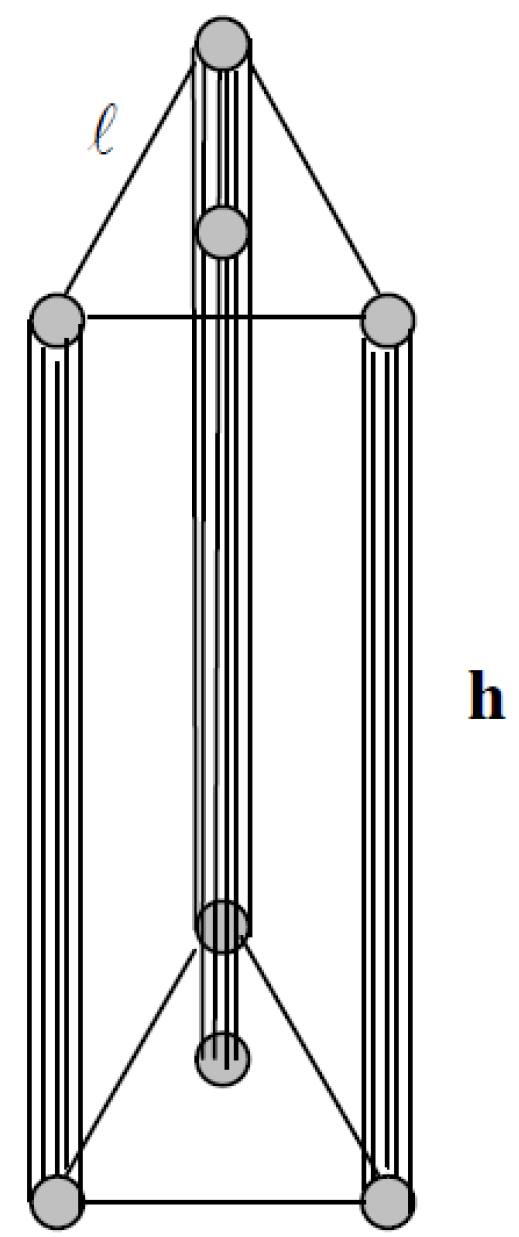
Figure 2.
Triangular prismatic representative volume element (RVE).

Figure 3.
Four-phase coaxial cylindrical model.

Figure 4.
Square body-centered prismatic model.
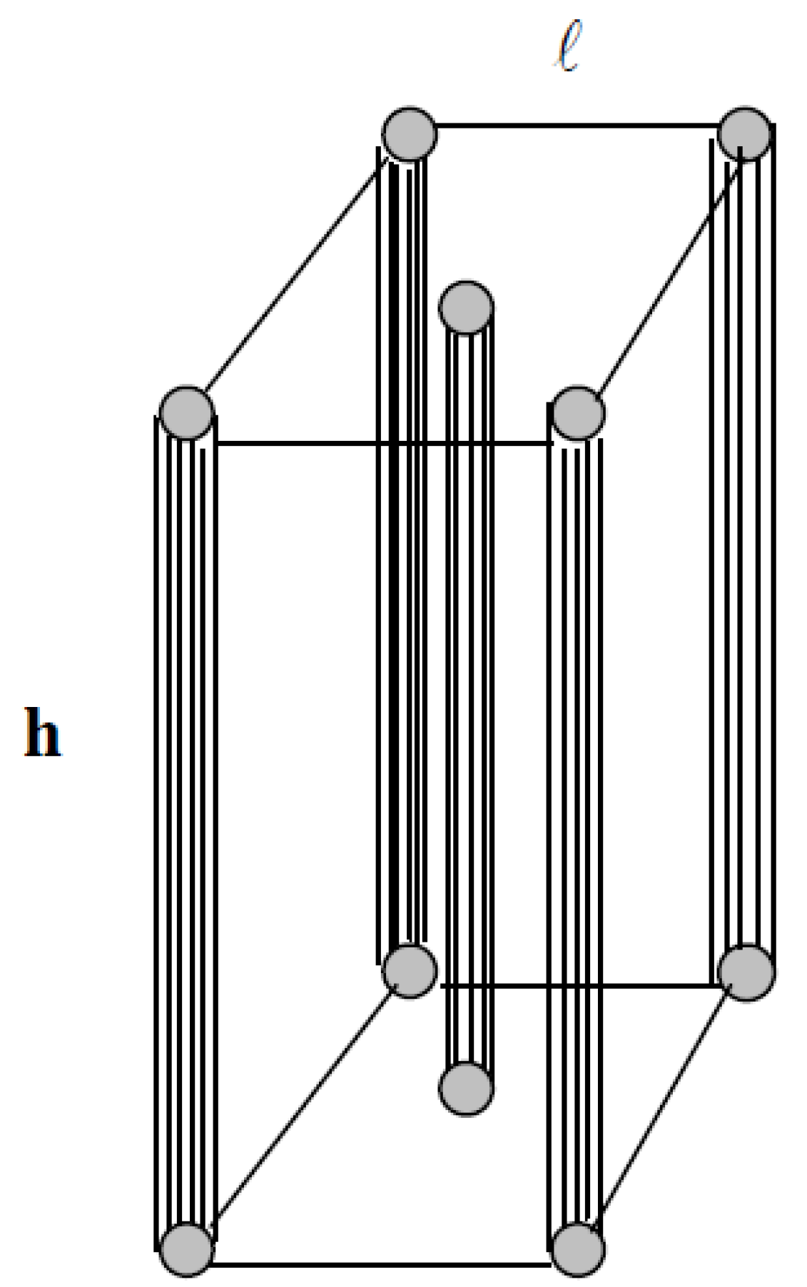
Figure 5.
Square prismatic RVE.
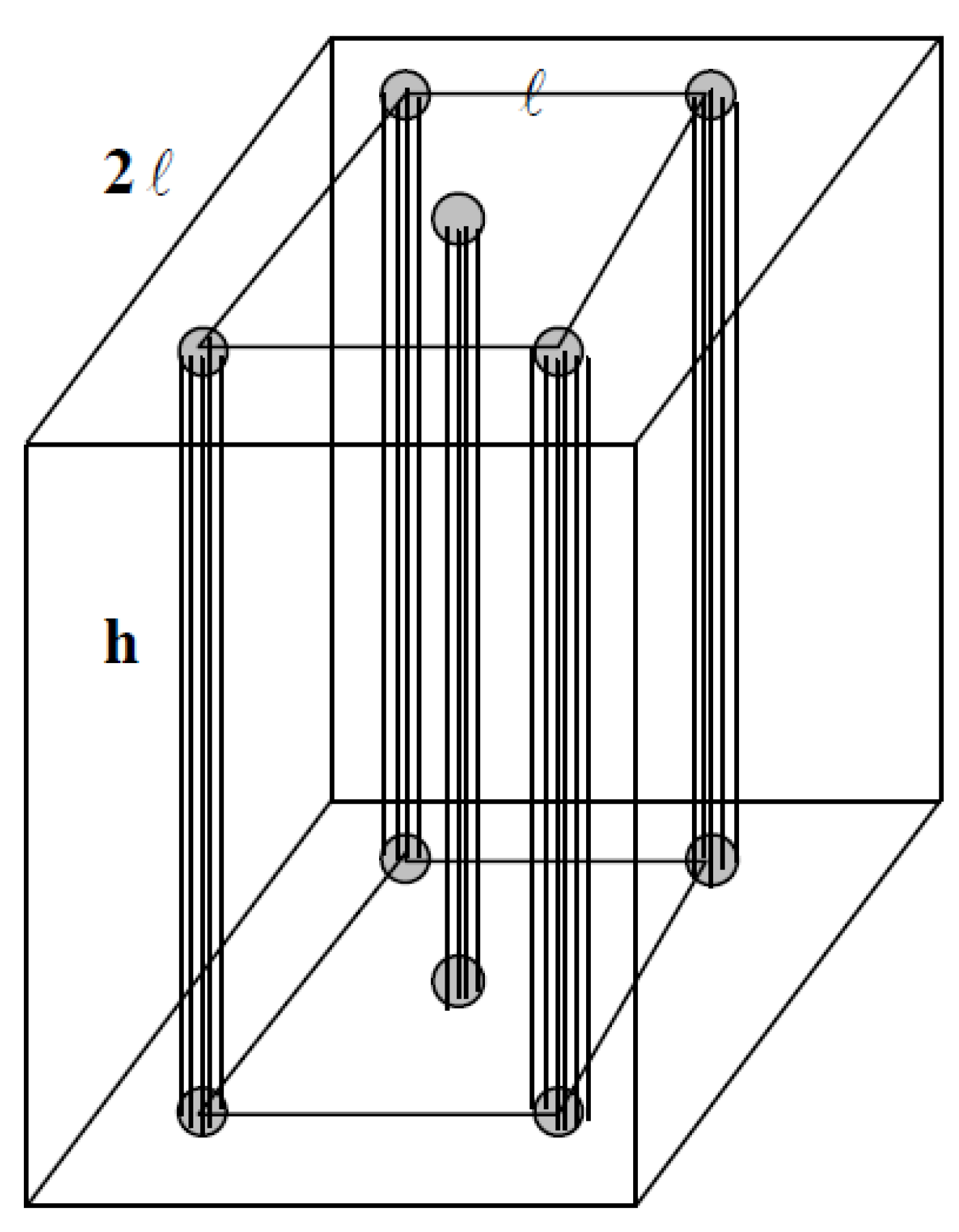
Figure 6.
Hexagonal body-centered prismatic model.

Figure 7.
Hexagonal prismatic RVE.
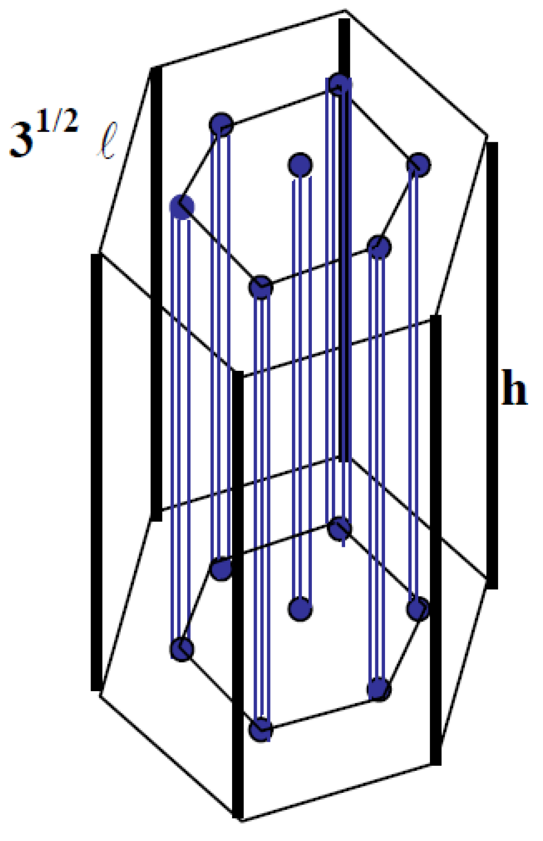
Figure 8.
Transformation of the three unit cells into a seven-phase cylindrical model, after the consideration of the interphase concept.
Figure 8.
Transformation of the three unit cells into a seven-phase cylindrical model, after the consideration of the interphase concept.

Figure 9.
Interphase content versus filler content.
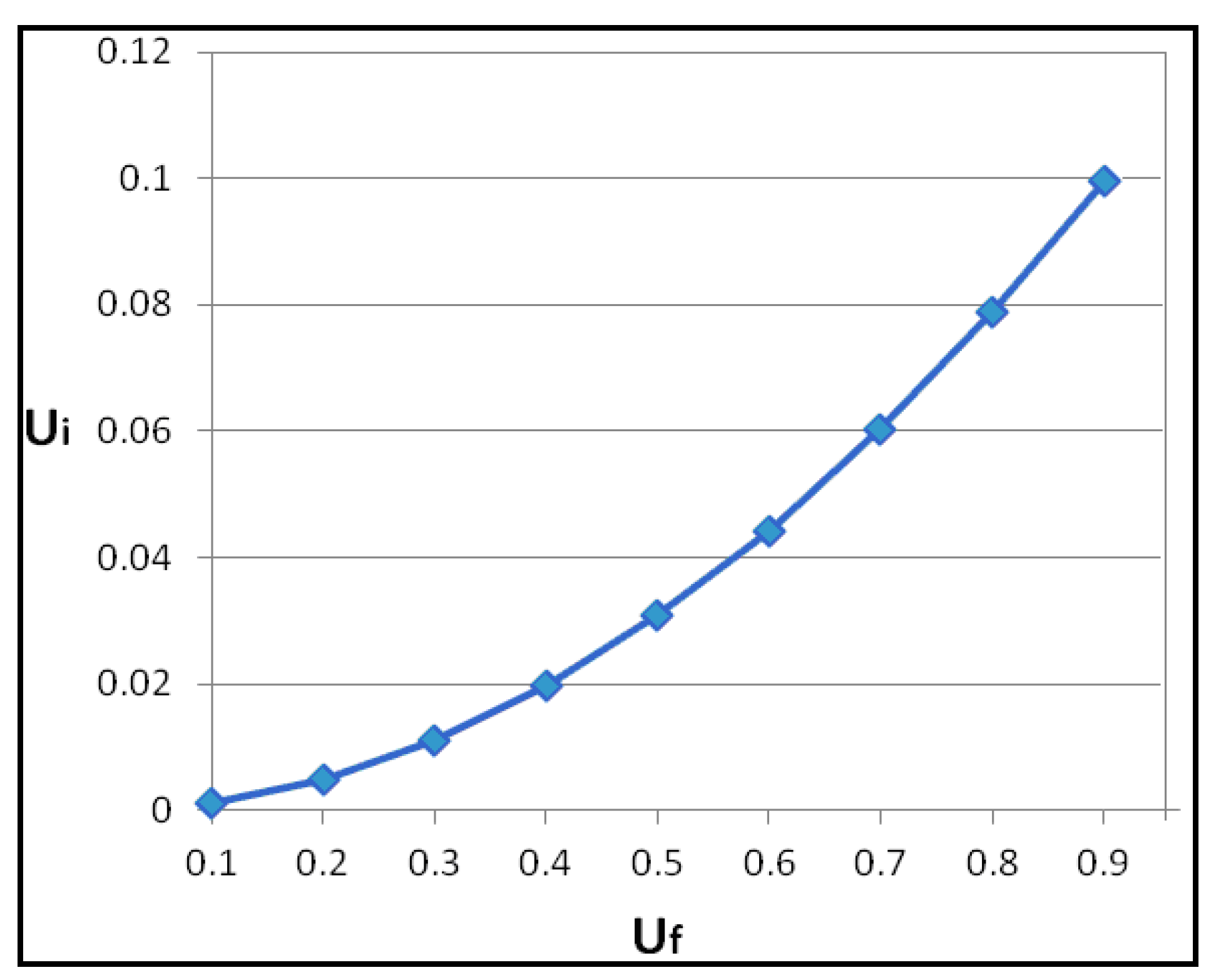
Figure 10.
Theoretical values of longitudinal thermal conductivity versus filler content.

Figure 11.
Theoretical values of transverse thermal conductivity versus filler content.

Table 1.
Radii of the seven-phase cylindrical model versus filler content.
| Uf | Ui | r1 (μm) | r2 (μm) | r3 (μm) | r4 (μm) | r5 (μm) | r6 (μm) | r7 (μm) |
|---|---|---|---|---|---|---|---|---|
| 0.10 | 0.0012 | 6 | 6.062 | 25.21 | 25.24 | 27.9 | 27.926 | 42.426 |
| 0.20 | 0.00492 | 6 | 6.127 | 16.74 | 16.79 | 20.62 | 20.692 | 30 |
| 0.30 | 0.01107 | 6 | 6.160 | 12.75 | 12.92 | 17.54 | 17.667 | 24.495 |
| 0.40 | 0.01968 | 6 | 6.181 | 10.28 | 10.38 | 15.77 | 15.976 | 21.213 |
| 0.50 | 0.03075 | 6 | 6.169 | 8.329 | 8.49 | 14.6 | 14.91 | 18.974 |
| 0.60 | 0.04428 | 6 | 6.084 | 6.770 | 6.85 | 13.77 | 14.211 | 17.321 |
| 0.65 | 0.052 | 6 | 6.007 | 6.053 | 6.08 | 13.44 | 13.964 | 16.641 |
Table 2.
Volume fractions of all phases.
| U1 | U2 | U3 | U4 | U5 | U6 | U7 |
|---|---|---|---|---|---|---|
| 0.02 | 0.0005 | 0.331 | 0.0005 | 0.08 | 0.00076 | 0.56674 |
| 0.04 | 0.0017 | 0.283 | 0.0019 | 0.14 | 0.00324 | 0.52426 |
| 0.06 | 0.0032 | 0.214 | 0.0035 | 0.22 | 0.00771 | 0.47979 |
| 0.08 | 0.0048 | 0.162 | 0.0051 | 0.32 | 0.01468 | 0.43282 |
| 0.10 | 0.0058 | 0.087 | 0.00569 | 0.411 | 0.02506 | 0.38244 |
| 0.12 | 0.0061 | 0.0286 | 0.0062 | 0.48 | 0.04068 | 0.32682 |
| 0.13 | 0.0075 | 0.002 | 0.0073 | 0.52 | 0.05163 | 0.29587 |
Table 3.
Longitudinal thermal conductivity of the composite for various filler contents.
| (W/mK) Equation (62) | (W/mK) Equation (63) | Rayleigh [1] | Springer-Tsai [4] | Clements and Moore Experiment Values [10] | Mutnuri Experiment Value [15] | |
|---|---|---|---|---|---|---|
| 0 | 0.2 | 0.2 | 0 | 0.2 | ||
| 0.1 | 0.192 | 0.329 | 0.22 | 0.3 | ||
| 0.2 | 0.208 | 0.441 | 0.44 | 0.4 | ||
| 0.3 | 0.248 | 0.573 | 0.66 | 0.5 | ||
| 0.4 | 0.312 | 0.687 | 0.88 | 0.6 | ||
| 0.5 | 0.4 | 0.796 | 1.1 | 0.7 | 0.471 | |
| 0.6 | 0.512 | 0.899 | 1.32 | 0.8 | 1.06 | |
| 0.65 | 0.577 | 0.970 | 1.43 | 0.85 | 1.14 |
Table 4.
Transverse thermal conductivity of the composite for various filler contents.
| Uf | (W/mK) Equation (65) | Two-Phase Inverse Mixtures Law | Springer-Tsai [4] | Hashin [3] | Clements and Moore Experiment Values [10] | Mutnuri Experiment Value [15] |
|---|---|---|---|---|---|---|
| 0 | 0.2 | 0.2 | 0.2 | 0.2 | ||
| 0.1 | 0.242 | 0.218 | 0.252 | 0.232 | ||
| 0.2 | 0.265 | 0.241 | 0.301 | 0.267 | ||
| 0.3 | 0.301 | 0.267 | 0.373 | 0.309 | ||
| 0.4 | 0.354 | 0.302 | 0.428 | 0.360 | ||
| 0.5 | 0.443 | 0.343 | 0.511 | 0.422 | 0.348 | |
| 0.6 | 0.522 | 0.411 | 0.592 | 0.501 | 0.55 | |
| 0.65 | 0.553 | 0.436 | 0.613 | 0.547 | 0.59 |
© 2017 by the authors. Licensee MDPI, Basel, Switzerland. This article is an open access article distributed under the terms and conditions of the Creative Commons Attribution (CC BY) license (http://creativecommons.org/licenses/by/4.0/).
Share and Cite
MDPI and ACS Style
Venetis, J.; Sideridis, E. The Thermal Conductivities of Periodic Fibrous Composites as Defined by a Mathematical Model. Fibers 2017, 5, 30. https://doi.org/10.3390/fib5030030
AMA Style
Venetis J, Sideridis E. The Thermal Conductivities of Periodic Fibrous Composites as Defined by a Mathematical Model. Fibers. 2017; 5(3):30. https://doi.org/10.3390/fib5030030
Chicago/Turabian StyleVenetis, John, and Emilio Sideridis. 2017. "The Thermal Conductivities of Periodic Fibrous Composites as Defined by a Mathematical Model" Fibers 5, no. 3: 30. https://doi.org/10.3390/fib5030030
Note that from the first issue of 2016, this journal uses article numbers instead of page numbers. See further details here.