A Measure of the Non-Determinacy of a Dynamic Neighborhood Model

Abstract

In this paper we define a non-deterministic dynamic neighborhood model. As a special case, a linear neighborhood model is considered. When a non-deterministic neighborhood model functions, it is possible to introduce a restriction on the number of active layers, which will allow the variation of the non-determinism of the model at each moment of time. We give the notion of the non-determinacy measure and prove that it has the properties of a probability measure. We formulate the problem of reachability with partially specified parameters, layer priorities, and the non-determinacy measure. An algorithm for solving the attainability problem for a neighborhood model with variable indeterminacy and layer priorities is presented. An example of its solution is shown, which shows that when the priorities are compared and the measure of non-determinism is used, the solution of the problem can be obtained more quickly than by a method that does not use priorities.

1. Introduction

Neighborhood models proposed by S.L. Blumin and A.M. Shmyrin in the late 1990s belong to the class of discrete systems and are used to model the behavior of complex spatially distributed objects.

The simplest class of neighborhood models is a symmetric linear neighborhood model for state and input and a linear mixed model for state, input, and output; the simplest class of nonlinear ones are bilinear neighborhood models for state and input [1,2].

In the theory of neighborhood systems, algorithms for parametric identification and mixed control for symmetric, mixed, and bilinear models have been developed [1,2].

A further direction in the development of the theory of neighborhood systems is fuzzy neighborhood models, which take into account the degree of fuzzy influence of neighborhood elements on each other [2].

It should be noted that the above neighborhood models are static and, therefore, applicable to modeling objects that do not change their state over time. However, the majority of real modeled objects are dynamic. An attempt to introduce dynamics into neighborhood models was made in linear neighborhood-time models [3].

The next stage in the development of the theory of neighborhood systems is the development and analysis of clear and fuzzy non-deterministic dynamic neighborhood models of Petri nets, allowing a fuzzy character of values in the nodes and of connections between the nodes of the system, as well as the development of identification algorithms and the solution of reachability problems with partially specified parameters for these classes of models [4,5]. Dynamic neighborhood models considered in References [4,5,6,7,8,9] are used to model the functioning of dynamic production systems.

Examples of the application of the method in question are the linear and bilinear neighborhood models of the wastewater treatment plant, the neighborhood model of transport systems, the model of the aeration tank functioning, and the dynamic non-deterministic neighborhood model of the functioning of cement production given in References [1,2,5].

In deterministic models, the process develops according to precisely defined rules. In this paper, we give the definition of non-deterministic dynamic neighborhood models in which there is some element of randomness of the system’s functioning and which make it possible to model stochastic parallel processes inherent in a significant part of production systems.

It should be noted that References [10,11] consider similar terms; however, unlike the present paper, they use agents moving along non-deterministic neighborhoods and interacting with each other. The models given in this paper differ by a layerwise assignment of the links between the nodes, while one or several layers (neighborhoods) are activated at a time according to the given statement, one of which is randomly selected for functioning.

In order to vary the non-determinacy of a neighborhood model, we introduce the notion of a non-determinacy measure. Let us consider the formulation, the algorithm, and an example of solving the problem of reaching a given state of a neighborhood model system with given layer priorities and a non-determinacy measure.

2. Dynamic Non-Deterministic Neighborhood Model

A dynamic neighborhood model can be specified by a set $\mathrm{N}{\mathrm{S}}_{\mathrm{D}}=\left(\mathrm{N},\mathrm{X},\mathrm{V},\mathrm{G},\mathrm{X}\left[0\right]\right)$ where:

• $\mathrm{N}=\left(\mathrm{A},{\mathrm{O}}_{\mathrm{x}},{\mathrm{O}}_{\mathrm{v}}\right)$—neighborhood model structure, $\mathrm{A}=\left\{{\mathrm{a}}_1,{\mathrm{a}}_2,\dots ,{\mathrm{a}}_{\mathrm{n}}\right\}$—set of nodes, ${\mathrm{O}}_{\mathrm{x}}$—neighborhoods of the nodes’ connections by states, ${\mathrm{O}}_{\mathrm{y}}$—neighborhoods of the nodes’ connections by controls, ${\mathrm{O}}_{\mathrm{y}}$—neighborhoods of the nodes’ connections by the output impact. For each node ${\mathrm{a}}_{\mathrm{i}}\in \mathrm{A}$, its own neighborhood is determined by states ${\mathrm{O}}_{\mathrm{x}}\left[{\mathrm{a}}_{\mathrm{i}}\right]\subseteq \mathrm{A}$, by controls ${\mathrm{O}}_{\mathrm{v}}\left[{\mathrm{a}}_{\mathrm{i}}\right]\subseteq \mathrm{A}$, and by outputs ${\mathrm{O}}_{\mathrm{y}}\left[{\mathrm{a}}_{\mathrm{i}}\right]\subseteq \mathrm{A}$; ${\mathrm{O}}_{\mathrm{x}}=\underset{\mathrm{i}=1}{\overset{\mathrm{n}}{\cup }}{\mathrm{O}}_{\mathrm{x}}\left[{\mathrm{a}}_{\mathrm{i}}\right]$, ${\mathrm{O}}_{\mathrm{v}}=\underset{\mathrm{i}=1}{\overset{\mathrm{n}}{\cup }}{\mathrm{O}}_{\mathrm{v}}\left[{\mathrm{a}}_{\mathrm{i}}\right]$; ${\mathrm{O}}_{\mathrm{y}}=\underset{\mathrm{i}=1}{\overset{\mathrm{n}}{\cup }}{\mathrm{O}}_{\mathrm{y}}\left[{\mathrm{a}}_{\mathrm{i}}\right]$;
• $\mathrm{X}\in {\mathrm{R}}^{\mathrm{n}}$—neighborhood model state vector in real time;
• $\mathrm{V}\in {\mathrm{R}}^{\mathrm{n}}$—neighborhood model input vector in real time;
• $\mathrm{G}:{\mathrm{X}}_{{\mathrm{O}}_{\mathrm{x}}}\times {\mathrm{V}}_{{\mathrm{O}}_{\mathrm{v}}}\to \mathrm{X}$—recalculation function of neighborhood model states (generally non-deterministic), where ${\mathrm{X}}_{{\mathrm{O}}_{\mathrm{x}}}$—number of node states entering the neighborhood ${\mathrm{O}}_{\mathrm{x}}$, ${\mathrm{V}}_{{\mathrm{O}}_{\mathrm{v}}}$—number of node controls entering the neighborhood ${\mathrm{O}}_{\mathrm{v}}$;
• $\mathrm{X}\left[0\right]$—initial state of the model.

In a dynamic non-deterministic neighborhood model, the neighborhoods of node connections by states and controls change over time. The whole set of connections between nodes $\mathrm{A}$ is divided into $\mathrm{m}$ sets of neighborhoods (layers) $\mathrm{O}[1],\mathrm{O}[2],\dots ,\mathrm{O}[\mathrm{m}]$. Each $\mathrm{k}$ layer $\left(\mathrm{k}=1,\dots ,\mathrm{m}\right)$ includes all nodes of the neighborhood model $\mathrm{A}=\left\{{\mathrm{a}}_1,{\mathrm{a}}_2,\dots ,{\mathrm{a}}_{\mathrm{n}}\right\}$ and part of the connections between them. The k-th layer is active at the time $\mathrm{t}$, if the specified activation ${\mathrm{f}}_{\mathrm{k}}[\mathrm{t}]=\mathrm{true}$ condition is met for it. At each current moment, several layers can be active, but only one of them is randomly selected for functioning.

A particular case of a neighborhood model is a linear one. In Reference [2], it was shown that the state recalculation function for a linear dynamic non-deterministic neighborhood model is set by an equation in the matrix form:

$$\begin{array}{l}\left[{\mathrm{W}}_{\mathrm{x}}^1\left[\mathrm{t}+1\right]{\mathrm{W}}_{\mathrm{x}}^2\left[\mathrm{t}+1\right]\dots {\mathrm{W}}_{\mathrm{x}}^{\mathrm{m}}\left[\mathrm{t}+1\right]\right]\cdot \mathrm{D}\left[\mathrm{t}\right]\cdot \mathrm{X}\left[\mathrm{t}+1\right]=\\ =\left[{\mathrm{W}}_{\mathrm{x}}^1\left[\mathrm{t}\right]{\mathrm{W}}_{\mathrm{x}}^2\left[\mathrm{t}\right]\dots {\mathrm{W}}_{\mathrm{x}}^{\mathrm{m}}\left[\mathrm{t}\right]\right]\cdot \mathrm{D}\left[\mathrm{t}\right]\cdot \mathrm{X}\left[\mathrm{t}\right]+\\ +\left[{\mathrm{W}}_{\mathrm{v}}^1\left[\mathrm{t}\right]{\mathrm{W}}_{\mathrm{v}}^2\left[\mathrm{t}\right]\dots {\mathrm{W}}_{\mathrm{v}}^{\mathrm{m}}\left[\mathrm{t}\right]\right]\cdot \mathrm{D}\left[\mathrm{t}\right]\cdot \mathrm{V}\left[\mathrm{t}\right]\end{array}$$

(1)

where ${\mathrm{W}}_{\mathrm{x}}^{\mathrm{k}}\left[\mathrm{t}+1\right]\in {\mathrm{R}}^{\mathrm{n}\times \mathrm{n}}$, ${\mathrm{W}}_{\mathrm{x}}^{\mathrm{k}}\left[\mathrm{t}\right]\in {\mathrm{R}}^{\mathrm{n}\times \mathrm{n}}$—matrices of the coefficients of the k-th layer by states at the moments $\mathrm{t}+1$ and $\mathrm{t}$, respectively; ${\mathrm{W}}_{\mathrm{v}}^{\mathrm{k}}\left[\mathrm{t}\right]\in {\mathrm{R}}^{\mathrm{n}\times \mathrm{n}}$—matrix of the coefficients of the k-th layer by inputs at the moment $\mathrm{t}$; $\mathrm{X}\left[\mathrm{t}+1\right]\in {\mathrm{R}}^{\mathrm{n}}$, $\mathrm{X}\left[\mathrm{t}\right]\in {\mathrm{R}}^{\mathrm{n}}$—state vector of the neighborhood system at the moments $\mathrm{t}+1$ and $\mathrm{t}$, respectively; $\mathrm{V}\left[\mathrm{t}\right]\in {\mathrm{R}}^{\mathrm{n}}$—input vector at the moment $\mathrm{t}$; $\mathrm{D}\left[\mathrm{t}\right]\in {\mathrm{R}}^{\mathrm{m}}$—random vector consisting of zeros and one unit in the position corresponding to the selected k-th layer, according to the equations of which the node states of the neighborhood model are recalculated at the next moment $\mathrm{t}+1$.

In Formula (1), the block matrix $[{\mathrm{W}}^1\left[\mathrm{t}\right]{\mathrm{W}}^2\left[\mathrm{t}\right]\dots {\mathrm{W}}^{\mathrm{m}}\left[\mathrm{t}\right]]$ is multiplied by the vector $\mathrm{D}\left[\mathrm{t}\right]={\left[\begin{array}{cccc}{\mathrm{d}}_1\left[\mathrm{t}\right]& {\mathrm{d}}_2\left[\mathrm{t}\right]& \dots & {\mathrm{d}}_{\mathrm{m}}\left[\mathrm{t}\right]\end{array}\right]}^{\mathrm{T}}$ according to the following rule: $\left[{\mathrm{W}}^1\left[\mathrm{t}\right]{\mathrm{W}}^2\left[\mathrm{t}\right]\dots {\mathrm{W}}^{\mathrm{m}}\left[\mathrm{t}\right]\right]\cdot \mathrm{D}\left[\mathrm{t}\right]={\displaystyle \sum _{\mathrm{k}=1}^{\mathrm{m}}{\mathrm{W}}^{\mathrm{k}}\left[\mathrm{t}\right]\cdot {\mathrm{d}}_{\mathrm{k}}\left[\mathrm{t}\right]}$.

3. The Concept of the Indeterminacy Measure

Before considering the following material, we give the definition of $\mathsf{\sigma }$-algebra. $\mathsf{\sigma }$-algebra is an algebra of sets which is closed under a countable union operation. $\mathsf{\sigma }$-algebras play an important role in the measure theory and the probability theory.

The family $\mathsf{\Phi }$ of subsets of the set $\mathsf{\Omega }$ is called sigma-algebra if it satisfies the following properties:

(1)

$\mathsf{\Phi }$ contains the set $\mathsf{\Omega }$.

(2)

If $\mathrm{A}\in \mathsf{\Phi }$, then its addition $\overline{\mathrm{A}}=\mathsf{\Omega }\backslash \mathrm{A}\in \mathsf{\Phi }$.

(3)

The union of a countable number of sets from $\mathsf{\Phi }$ also belongs to $\mathsf{\Phi }$.

In the functioning of a non-deterministic neighborhood model, it is possible to introduce a limitation on the number of active layers, which will allow the variation of the non-determinism of a model at each moment $\mathrm{t}$. We introduce the notion of the measure of the non-determinacy of a neighborhood model [2,3].

Let $\mathsf{\Omega }$ be the set of all layers of a neighborhood model, and $\mathsf{\Phi }$ be the set of all subsets $\mathsf{\Phi }$, including $Ø$.

Theorem 1.

$\mathsf{\Phi }$ is $\mathsf{\sigma }$-algebra.

Proof 

• $\mathsf{\Omega }\in \mathsf{\Phi }$ (by the definition of set $\mathsf{\Phi }$) is satisfied.
• If $\mathrm{A}\in \mathsf{\Phi }$, then $\overline{\mathrm{A}}=\mathsf{\Omega }\backslash \mathrm{A}\in \mathsf{\Phi }$ (by definition of set $\mathsf{\Phi }$) is satisfied.
• If ${\mathrm{A}}_1,{\mathrm{A}}_2,\dots \in \mathsf{\Phi }$, then ${\mathrm{A}}_1\cup {\mathrm{A}}_2\cup \dots \in \mathsf{\Phi }$ (also by definition of set $\mathsf{\Phi }$) is satisfied.

Hence, is $\mathsf{\Phi }$—$\mathsf{\sigma }$-algebra. □

The number of elements of any set $\mathrm{A}\in \mathsf{\Phi }$ will be called the potency of the set $\mathrm{A}$ and denoted by $\left|\mathrm{A}\right|$. Obviously, $|Ø|=0$—the potency of the empty set is zero, $\left|\mathsf{\Omega }\right|=\mathrm{m}$—the potency of the set $\mathsf{\Omega }$ is equal to the number of layers of the neighborhood model.

We call the measure of the non-determinacy of the neighborhood model the function: $\mathrm{g}:\mathsf{\Phi }\to \left[0,1\right]$: $\forall \mathrm{A}\in \mathsf{\Phi }\mathrm{g}\left(\mathrm{A}\right)=\left|\mathrm{A}\right|/\left|\mathsf{\Omega }\right|=\mathrm{h}/\mathrm{m}$, where $\mathrm{h}$—the potency of the set $\mathrm{A}$.

Theorem 2.

$\mathrm{g}$ has the properties of a probability measure.

Proof 

• For any $\mathrm{A}\in \mathsf{\Phi }$ $\mathrm{g}\left(\mathrm{A}\right)\ge 0$, it is satisfied by the definition of the function $\mathrm{g}$.
• For any countable collection of sets ${\mathrm{A}}_1,{\mathrm{A}}_2,\dots \in \mathsf{\Phi }$ such that ${\mathrm{A}}_1\cap {\mathrm{A}}_2\cap \dots =Ø$, the equation: $\mathrm{g}\left(\underset{\mathrm{i}=1}{\overset{\infty }{\cup }}{\mathrm{A}}_{\mathrm{i}}\right)={\displaystyle \sum _{\mathrm{i}=1}^{\infty }\mathrm{g}\left({\mathrm{A}}_{\mathrm{i}}\right)}$ is satisfied.
  Indeed, let ${\mathrm{A}}_1,{\mathrm{A}}_2,\dots \in \mathsf{\Phi }$, $\left|{\mathrm{A}}_1\right|={\mathrm{h}}_1,\left|{\mathrm{A}}_2\right|={\mathrm{h}}_2,\dots$, and ${\mathrm{A}}_1\cap {\mathrm{A}}_2\cap \dots =Ø$. Then $\left|\underset{\mathrm{i}=1}{\overset{\infty }{\cup }}{\mathrm{A}}_{\mathrm{i}}\right|={\mathrm{h}}_1+{\mathrm{h}}_2+\dots$; $\mathrm{g}\left(\underset{\mathrm{i}=1}{\overset{\infty }{\cup }}{\mathrm{A}}_{\mathrm{i}}\right)=\frac{{\mathrm{h}}_1+{\mathrm{h}}_2+\dots }{\mathrm{m}}$.
  $\mathrm{g}\left({\mathrm{A}}_1\right)=\frac{{\mathrm{h}}_1}{\mathrm{m}}$, $\mathrm{g}\left({\mathrm{A}}_2\right)=\frac{{\mathrm{h}}_2}{\mathrm{m}}$, … $\Rightarrow$ ${\displaystyle \sum _{\mathrm{i}=1}^{\infty }\mathrm{g}\left({\mathrm{A}}_{\mathrm{i}}\right)}=\frac{{\mathrm{h}}_1}{\mathrm{m}}+\frac{{\mathrm{h}}_2}{\mathrm{m}}+\dots =\frac{{\mathrm{h}}_1+{\mathrm{h}}_2+\dots }{\mathrm{m}}$.
  Consequently, $\mathrm{g}\left(\underset{\mathrm{i}=1}{\overset{\infty }{\cup }}{\mathrm{A}}_{\mathrm{i}}\right)={\displaystyle \sum _{\mathrm{i}=1}^{\infty }\mathrm{g}\left({\mathrm{A}}_{\mathrm{i}}\right)}$.
• $\mathrm{g}\left(\mathsf{\Omega }\right)=1$ is satisfied. Indeed, $\mathrm{g}\left(\mathsf{\Omega }\right)=\frac{\mathrm{m}}{\mathrm{m}}=1$.

Thus, the function $\mathrm{g}$ is a probability measure. □

Let the sets ${\mathrm{A}}_0,{\mathrm{A}}_1,{\mathrm{A}}_2\dots$ be active layers of a non-deterministic neighborhood model at the moments $\mathrm{t}=0,1,2,\dots$, then $\mathrm{g}\left({\mathrm{A}}_0\right),\mathrm{g}\left({\mathrm{A}}_1\right),\mathrm{g}\left({\mathrm{A}}_2\right)\dots$ will be called the non-determinacy measure ${\mathrm{g}}_{\mathrm{t}}$ of the neighborhood model, respectively, at the moments $\mathrm{t}=0,1,2,\dots$. The more active layers at each moment, the greater the non-determinacy measure of the neighborhood model. By introducing a restriction on the number of active layers, it is possible to change the non-determinacy measure and to regulate the process of functioning of a non-deterministic neighborhood model.

4. The Reachability Problem with Partially Specified Parameters, Layer Priorities, and the Non-Determinacy Measure

Let the initial state $\mathrm{X}[0]$ be given at the initial moment of the neighborhood model functioning.

Let ${\mathrm{X}}^{\ast }\in {\mathrm{R}}^{\mathrm{n}}$ be the state of the neighborhood model which it must reach as a result of functioning, the vector ${\mathrm{D}}^{\ast }\in {\mathrm{R}}^{\mathrm{m}}$ is the sum of control actions that transfer the initial state $\mathrm{X}[0]$ of the neighborhood model into the state ${\mathrm{X}}^{\ast }$, while only a part of the coordinates of the state vector ${\mathrm{X}}^{\ast }$ and the sum vector of the controls ${\mathrm{D}}^{\ast }$ is known.

Each layer $\mathrm{k}$ $(\mathrm{k}=1,\dots ,\mathrm{m})$ of the neighborhood model is given priority ${\mathrm{w}}_{\mathrm{k}}\in [0,1]$ by experts. The non-determinacy measure $\mathrm{g}$ of the model is given.

Taking into account the priorities of the layers and the non-determinacy measure of the model, it is required to determine the unknown components of the state vector ${\mathrm{X}}^{\ast }$ and the sum of controls vector ${\mathrm{D}}^{\ast }$, as well as the sequence of control actions at each moment of the model’s functioning $\mathrm{D}[0],\mathrm{D}[1],\dots$ that transfer the initial state $\mathrm{X}[0]$ into the state ${\mathrm{X}}^{\ast }$.

In order to solve the reachability problem for the considered neighborhood model, the following criterion can be used:

$$\mathrm{K}\left(\mathrm{X}[\mathrm{t}+1],\mathrm{D}\mathrm{t}\right)=\sqrt{{\displaystyle \sum _{\mathrm{i}=1}^{{\mathrm{N}}_{\mathrm{X}}}{\left(\frac{{\mathrm{x}}_{\mathrm{i}}\left[\mathrm{t}+1\right]-{\mathrm{x}}_{\mathrm{i}}^{\ast }}{{\mathrm{x}}_{\mathrm{i}}^{\ast }}\right)}^2}+{\displaystyle \sum _{\mathrm{j}=1}^{{\mathrm{N}}_{\mathrm{D}}}{\left(\frac{\mathrm{d}{\mathrm{t}}_{\mathrm{j}}-{\mathrm{d}}_{\mathrm{j}}^{\ast }}{{\mathrm{d}}_{\mathrm{j}}^{\ast }}\right)}^2}}\to \min$$

(2)

where $\mathrm{t}=0,\dots ,\mathrm{T}-1$; ${\mathrm{x}}_{\mathrm{i}}\left[\mathrm{t}+1\right]$ $\left(\mathrm{i}=1,\dots ,{\mathrm{N}}_{\mathrm{X}}\right)$—unknown state components $\mathrm{X}[\mathrm{t}+1]$ at the moment $\mathrm{t}+1$; ${\mathrm{x}}_{\mathrm{i}}^{\ast }$—nominal values of the state component; ${\mathrm{N}}_{\mathrm{X}}$—number of specified state components ${\mathrm{X}}^{\ast }$; $\mathrm{d}{\mathrm{t}}_{\mathrm{j}}$ $\left(\mathrm{j}=1,\dots ,{\mathrm{N}}_{\mathrm{D}}\right)$—vector coordinates $\mathrm{D}\mathrm{t}$; ${\mathrm{d}}_{\mathrm{j}}^{\ast }$—nominal values of control components; $\mathrm{T}$—maximum number of the model functioning strokes. Nominal values and $\mathrm{T}$ can be set by experts.

It is necessary to obtain the minimum value of the functional $\mathrm{K}\left(\mathrm{X}[\mathrm{t}+1],\mathrm{D}\mathrm{t}\right)$ for a given number of strokes $\mathrm{T}$ of dynamic neighborhood model functioning, taking into account the priorities of the layers and the non-determinacy measure.

Let us consider step by step the algorithm for solving the reachability problem for a dynamic non-deterministic neighborhood model with given layer priorities and a non-determinacy measure.

• Set the initial state $\mathrm{X}[0]$, input impacts $\mathrm{V}[\mathrm{t}]$, part of the state vector coordinates ${\mathrm{X}}^{\ast }$ and the control vector ${\mathrm{D}}^{\ast }$, the maximum number of strokes $\mathrm{T}$ of dynamic neighborhood model functioning, and solution accuracy $\mathsf{\epsilon }>0$.
• Set the priorities of the model layers ${\mathrm{w}}_{\mathrm{k}}\in [0,1]$ $(\mathrm{k}=1,\dots ,\mathrm{m})$. Specify the model’s non-determinacy measure $\mathrm{g}\in [0,1]$.
• Model functioning time is $\mathrm{t}=0$. Control $\mathrm{D}\mathrm{t}=0$.
• Let $\mathrm{X}[0]$ be the root of the state tree and the current element of the tree.
• The minimum value of the functional ${\mathrm{K}}_{\min }:=\infty$. The optimal path corresponding to ${\mathrm{K}}_{\min }$ is ${\mathrm{P}}_{{\mathrm{K}}_{\min }}:=Ø$.
• Find the set of active layers ${\mathrm{A}}_{\mathrm{t}}$ of the model at the moment $\mathrm{t}$; $\mathrm{q}[\mathrm{t}]:=\left|{\mathrm{A}}_{\mathrm{t}}\right|$—the potency of the set ${\mathrm{A}}_{\mathrm{t}}$.
• In accordance with the measure $\mathrm{g}$, find the subset ${\mathrm{B}}_{\mathrm{t}}$ of the set ${\mathrm{A}}_{\mathrm{t}}$, while in the set ${\mathrm{B}}_{\mathrm{t}}$ layers from ${\mathrm{A}}_{\mathrm{t}}$ are selected in order of decreasing priority. $\mathrm{q}[\mathrm{t}]:=\left|{\mathrm{B}}_{\mathrm{t}}\right|$ is the potency of the set ${\mathrm{B}}_{\mathrm{t}}$.
• If $\mathrm{q}[\mathrm{t}]=0$, $\mathrm{t}=\mathrm{T}+1$. Go to step 12. Otherwise go to step 9.
• Let the layers $\mathrm{O}[{\mathrm{j}}_1],\dots ,\mathrm{O}[{\mathrm{j}}_{\mathrm{q}[\mathrm{t}]}]$, ${\mathrm{j}}_1,\dots ,{\mathrm{j}}_{\mathrm{q}}\in \left\{1,\dots ,\mathrm{m}\right\}$ be active at the moment $\mathrm{t}$. Reverse the elements $\mathrm{O}[{\mathrm{j}}_1],\dots ,\mathrm{O}[{\mathrm{j}}_{\mathrm{q}[\mathrm{t}]}]$ of the set of active layers ${\mathrm{B}}_{\mathrm{t}}$ and correspondingly, to each element $\mathrm{O}\left[{\mathrm{j}}_{\mathrm{k}}\right]$ form a vector ${\mathrm{D}}^{{\mathrm{j}}_{\mathrm{k}}}\left[\mathrm{t}\right]$. For the active layer $\mathrm{O}\left[{\mathrm{j}}_{\mathrm{k}}\right]$, the components of the vector ${\mathrm{D}}^{{\mathrm{j}}_{\mathrm{k}}}\left[\mathrm{t}\right]$ are:

  $${\mathrm{d}}_{\mathrm{u}}^{{\mathrm{j}}_{\mathrm{k}}}[\mathrm{t}]=\{\begin{array}{ll}1,\hfill & \mathrm{u}={\mathrm{j}}_{\mathrm{k}}\\ 0,\hfill & \mathrm{u}\ne {\mathrm{j}}_{\mathrm{k}}\end{array},\mathrm{u}=1,\dots ,\mathrm{m}.$$
• For each vector ${\mathrm{D}}^{{\mathrm{j}}_{\mathrm{k}}}\left[\mathrm{t}\right]$, use the pseudo-inversion to solve the equation:

  $$\begin{array}{l}\left[{\mathrm{W}}_{\mathrm{x}}^1\left[\mathrm{t}+1\right]{\mathrm{W}}_{\mathrm{x}}^2\left[\mathrm{t}+1\right]\dots {\mathrm{W}}_{\mathrm{x}}^{\mathrm{m}}\left[\mathrm{t}+1\right]\right]\cdot {\mathrm{D}}^{{\mathrm{j}}_{\mathrm{k}}}\left[\mathrm{t}\right]\cdot {\mathrm{X}}^{{\mathrm{j}}_{\mathrm{k}}}\left[\mathrm{t}+1\right]=\\ =\left[{\mathrm{W}}_{\mathrm{x}}^1\left[\mathrm{t}\right]{\mathrm{W}}_{\mathrm{x}}^2\left[\mathrm{t}\right]\dots {\mathrm{W}}_{\mathrm{x}}^{\mathrm{m}}\left[\mathrm{t}\right]\right]\cdot {\mathrm{D}}^{{\mathrm{j}}_{\mathrm{k}}}\left[\mathrm{t}\right]\cdot \mathrm{X}\left[\mathrm{t}\right]+\\ +\left[{\mathrm{W}}_{\mathrm{v}}^1\left[\mathrm{t}\right]{\mathrm{W}}_{\mathrm{v}}^2\left[\mathrm{t}\right]\dots {\mathrm{W}}_{\mathrm{v}}^{\mathrm{m}}\left[\mathrm{t}\right]\right]\cdot {\mathrm{D}}^{{\mathrm{j}}_{\mathrm{k}}}\left[\mathrm{t}\right]\cdot \mathrm{V}\left[\mathrm{t}\right]\end{array}$$

  and find ${\mathrm{X}}^{{\mathrm{j}}_{\mathrm{k}}}[\mathrm{t}+1]$. For each state ${\mathrm{X}}^{{\mathrm{j}}_{\mathrm{k}}}[\mathrm{t}+1]$ and control $\mathrm{D}\mathrm{t}=\mathrm{D}\mathrm{t}+{\mathrm{D}}^{{\mathrm{j}}_{\mathrm{k}}}\left[\mathrm{t}\right]$, calculate and store the value of the functional (2) $\mathrm{K}({\mathrm{X}}^{{\mathrm{j}}_{\mathrm{k}}}[\mathrm{t}+1],\mathrm{D}\mathrm{t})$. The path leading to this state is $\mathrm{P}({\mathrm{X}}^{{\mathrm{j}}_{\mathrm{k}}}[\mathrm{t}+1])=\mathrm{P}(\mathrm{X}[\mathrm{t}])\cup {\mathrm{j}}_{\mathrm{k}}$.
• If for some state ${\mathrm{X}}^{{\mathrm{j}}_{\mathrm{k}}}[\mathrm{t}+1]$ the value of the functional is $\mathrm{K}({\mathrm{X}}^{{\mathrm{j}}_{\mathrm{k}}}[\mathrm{t}+1],\mathrm{D}\mathrm{t})<\mathsf{\epsilon }$, then the optimal control $\mathrm{D}\mathrm{t}$ is found providing the optimal solution ${\mathrm{X}}^{{\mathrm{j}}_{\mathrm{k}}}[\mathrm{t}+1]$ with accuracy $\mathsf{\epsilon }$ at ${\mathrm{K}}_{\min }=\mathrm{K}({\mathrm{X}}^{{\mathrm{j}}_{\mathrm{k}}}[\mathrm{t}+1],\mathrm{D}\mathrm{t})$. The corresponding optimal path is ${\mathrm{P}}_{{\mathrm{K}}_{\min }}=\mathrm{P}({\mathrm{X}}^{{\mathrm{j}}_{\mathrm{k}}}[\mathrm{t}+1])$. End of algorithm. Otherwise go to item 12.
• If $\mathrm{t}+1>\mathrm{T}$, then the maximum depth of the tree is reached. In the resulting tree, find the state that gives the minimum value of the functional (2) ${\mathrm{K}}_{\min }$, the corresponding control, and the path leading to this state. The solution is called quasi-optimal. Otherwise go to step 13.
• Add the states ${\mathrm{X}}^{{\mathrm{j}}_1}[\mathrm{t}+1],\dots ,{\mathrm{X}}^{{\mathrm{j}}_{\mathrm{q}[\mathrm{t}]}}[\mathrm{t}+1]$ as descendants to the current state tree element. Remember for each ${\mathrm{X}}^{{\mathrm{j}}_{\mathrm{k}}}[\mathrm{t}+1]$ $(\mathrm{k}=1,\dots ,\mathrm{q}[\mathrm{t}])$ the value of the functional (2), control $\mathrm{D}\mathrm{t}$, and path ${\mathrm{P}}_{{\mathrm{K}}_{\min }}$ leading to this state. For each ${\mathrm{X}}^{{\mathrm{j}}_{\mathrm{k}}}[\mathrm{t}+1]$ $(\mathrm{k}=1,\dots ,\mathrm{q}[\mathrm{t}])$ perform the algorithm, starting with step 6, at $\mathrm{t}=\mathrm{t}+1$.

In order to obtain a more accurate solution, it is necessary to increase the number of strokes $\mathrm{T}$ of dynamic neighborhood model functioning.

It should be noted that this algorithm provides an optimal solution until a certain value of the non-determinacy measure. With a significant decrease in the non-determinacy measure, only a quasi-optimal solution can be obtained, since the number of active layers decreases simultaneously at each moment of time, and some states of the system become unattainable.

5. An Example of Solving the Reachability Problem with Given Priorities of Layers and a Non-Determinacy Measure

Let a non-deterministic neighborhood model be given consisting of four nodes $\mathrm{A}=\{1,2,3,4\}$ and three layers specified by the neighborhoods $\mathrm{O}(1),\mathrm{O}(2),\mathrm{O}(3)$.

$$\begin{array}{l}{\mathrm{O}}_{\mathrm{x}}(1)=\{{\mathrm{O}}_{\mathrm{x}}[1]={\mathrm{O}}_{\mathrm{v}}[1]=\{1\};{\mathrm{O}}_{\mathrm{x}}[2]={\mathrm{O}}_{\mathrm{v}}[2]=\{1,2\};\\ {\mathrm{O}}_{\mathrm{x}}[3]={\mathrm{O}}_{\mathrm{v}}[3]=\left\{3\right\};{\mathrm{O}}_{\mathrm{x}}[4]={\mathrm{O}}_{\mathrm{v}}[4]=\left\{4\right\}\};\end{array}$$

$$\begin{array}{l}{\mathrm{O}}_{\mathrm{x}}(2)=\{{\mathrm{O}}_{\mathrm{x}}[1]={\mathrm{O}}_{\mathrm{v}}[1]=\{1\};{\mathrm{O}}_{\mathrm{x}}[2]={\mathrm{O}}_{\mathrm{v}}[2]=\{2\};\\ {\mathrm{O}}_{\mathrm{x}}[3]={\mathrm{O}}_{\mathrm{v}}[3]=\{1,3\};{\mathrm{O}}_{\mathrm{x}}[4]={\mathrm{O}}_{\mathrm{v}}[4]=\left\{4\right\}\};\end{array}$$

$$\begin{array}{l}{\mathrm{O}}_{\mathrm{x}}(3)=\{{\mathrm{O}}_{\mathrm{x}}[1]={\mathrm{O}}_{\mathrm{v}}[1]=\{1\};{\mathrm{O}}_{\mathrm{x}}[2]={\mathrm{O}}_{\mathrm{v}}[2]=\{2\};\\ {\mathrm{O}}_{\mathrm{x}}[3]={\mathrm{O}}_{\mathrm{v}}[3]=\left\{3\right\};{\mathrm{O}}_{\mathrm{x}}[4]={\mathrm{O}}_{\mathrm{v}}[4]=\{2,3,4\}\}.\end{array}$$

The structure of the neighborhood model is shown in Figure 1.

Let the input impacts on each layer be constant:

$${\mathrm{V}}_1\left[\mathrm{t}\right]=\left[\begin{array}{c}-1\\ 1\\ 0\\ 0\end{array}\right],{\mathrm{V}}_2\left[\mathrm{t}\right]=\left[\begin{array}{c}-1\\ 0\\ 1\\ 0\end{array}\right],{\mathrm{V}}_3\left[\mathrm{t}\right]=\left[\begin{array}{c}0\\ -1\\ -1\\ 1\end{array}\right]$$

After identification, the following systems of equations are obtained. For the first layer:

$$\{\begin{array}{l}{\mathrm{x}}_1\left[\mathrm{t}+1\right]+{\mathrm{x}}_2\left[\mathrm{t}+1\right]={\mathrm{x}}_1\left[\mathrm{t}\right]+{\mathrm{x}}_2\left[\mathrm{t}\right]+{\mathrm{v}}_1\left[\mathrm{t}\right]+{\mathrm{v}}_2\left[\mathrm{t}\right];\hfill \\ {\mathrm{x}}_2\left[\mathrm{t}+1\right]={\mathrm{x}}_2\left[\mathrm{t}\right]+{\mathrm{v}}_2\left[\mathrm{t}\right];\hfill \\ {\mathrm{x}}_3\left[\mathrm{t}+1\right]={\mathrm{x}}_3\left[\mathrm{t}\right]+{\mathrm{v}}_3\left[\mathrm{t}\right];\hfill \\ {\mathrm{x}}_4\left[\mathrm{t}+1\right]={\mathrm{x}}_4\left[\mathrm{t}\right]+{\mathrm{v}}_4\left[\mathrm{t}\right].\hfill \end{array}$$

For the second layer:

$$\{\begin{array}{l}{\mathrm{x}}_1\left[\mathrm{t}+1\right]+{\mathrm{x}}_3\left[\mathrm{t}+1\right]={\mathrm{x}}_1\left[\mathrm{t}\right]+{\mathrm{x}}_3\left[\mathrm{t}\right]+{\mathrm{v}}_1\left[\mathrm{t}\right]+{\mathrm{v}}_3\left[\mathrm{t}\right];\hfill \\ {\mathrm{x}}_2\left[\mathrm{t}+1\right]={\mathrm{x}}_2\left[\mathrm{t}\right]+{\mathrm{v}}_2\left[\mathrm{t}\right];\hfill \\ {\mathrm{x}}_3\left[\mathrm{t}+1\right]={\mathrm{x}}_3\left[\mathrm{t}\right]+{\mathrm{v}}_3\left[\mathrm{t}\right];\hfill \\ {\mathrm{x}}_4\left[\mathrm{t}+1\right]={\mathrm{x}}_4\left[\mathrm{t}\right]+{\mathrm{v}}_4\left[\mathrm{t}\right].\hfill \end{array}$$

For the third layer:

$$\{\begin{array}{l}{\mathrm{x}}_1\left[\mathrm{t}+1\right]={\mathrm{x}}_1\left[\mathrm{t}\right]+{\mathrm{v}}_1\left[\mathrm{t}\right];\hfill \\ {\mathrm{x}}_2\left[\mathrm{t}+1\right]+{\mathrm{x}}_4\left[\mathrm{t}+1\right]={\mathrm{x}}_2\left[\mathrm{t}\right]+{\mathrm{x}}_4\left[\mathrm{t}\right]+{\mathrm{v}}_2\left[\mathrm{t}\right]+{\mathrm{v}}_4\left[\mathrm{t}\right];\hfill \\ {\mathrm{x}}_3\left[\mathrm{t}+1\right]+{\mathrm{x}}_4\left[\mathrm{t}+1\right]={\mathrm{x}}_3\left[\mathrm{t}\right]+{\mathrm{x}}_4\left[\mathrm{t}\right]+{\mathrm{v}}_3\left[\mathrm{t}\right]+{\mathrm{v}}_4\left[\mathrm{t}\right];\hfill \\ {\mathrm{x}}_4\left[\mathrm{t}+1\right]={\mathrm{x}}_4\left[\mathrm{t}\right]+{\mathrm{v}}_4\left[\mathrm{t}\right].\hfill \end{array}$$

We introduce the priorities of the layers: ${\mathrm{w}}_1=0,1$; ${\mathrm{w}}_2=0,7$; ${\mathrm{w}}_3=0,5$.

Let $\mathrm{X}[0]=\left[\begin{array}{l}2\hfill \\ 3\hfill \\ 1\hfill \\ 0\hfill \end{array}\right]$, ${\mathrm{X}}^{\ast }=\left[\begin{array}{l}\\ \\ \\ 3\hfill \end{array}\right]$, ${\mathrm{D}}^{\ast }=\left[\begin{array}{l}\\ \\ 3\hfill \end{array}\right]$; $\mathrm{g}=\frac{2}{3}$; $\mathsf{\epsilon }=0,1$.

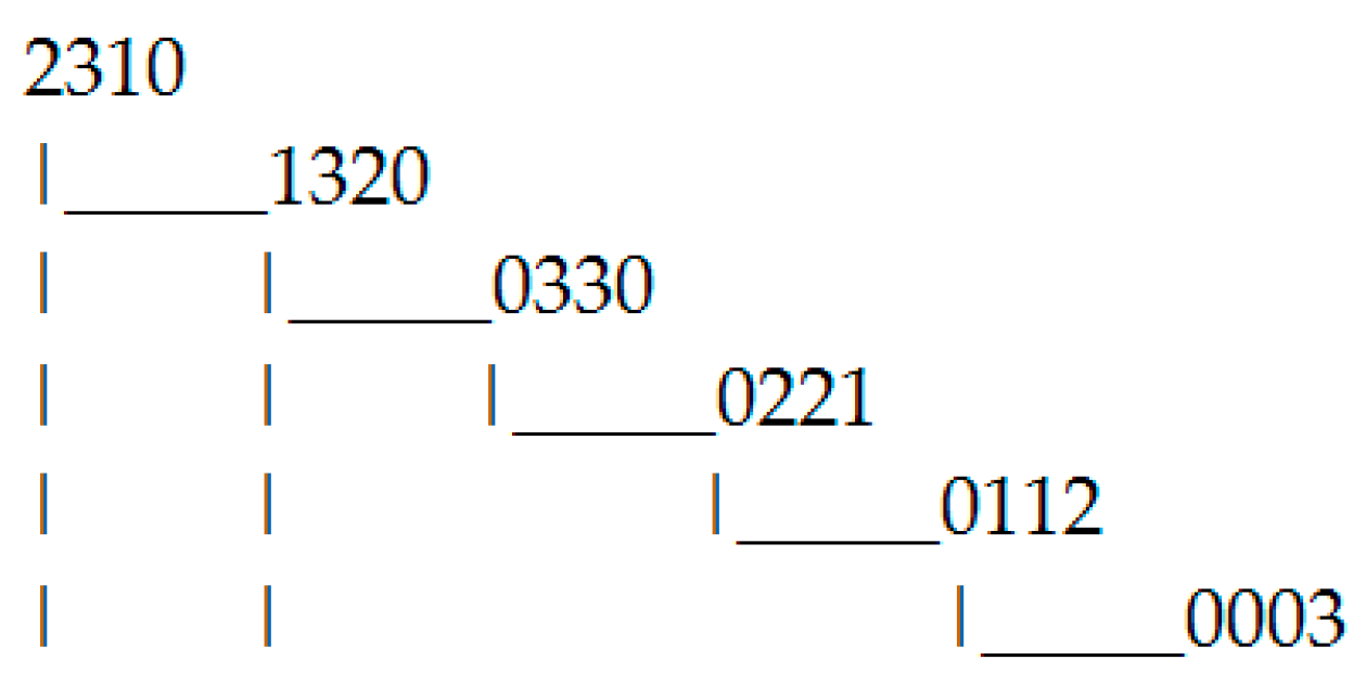
Let us construct a state tree taking into account the priorities (Figure 2).

For each found state and its corresponding control, we find the value of the functional (2) and write it into

Table 1. The values of the functional (2) for the neighborhood model in Figure 1, taking into account the priorities.

$\mathbf{t}$	$\mathbf{X}\left[\mathbf{t}+1\right]$				$\mathbf{D}\mathbf{t}$			$\mathbf{K}$
0	1	3	2	0	0	1	0	1.414214
1	0	3	3	0	0	2	0	1.414214
2	0	2	2	1	0	2	1	0.942809
3	0	1	1	2	0	2	2	0.471405
4	0	0	0	3	0	2	3	0

.

Thus, the optimal solution giving the minimal value of the functional (2) ${\mathrm{K}}_{\min }=0$ is $\mathrm{X}[5]={[0,0,0,3]}^{\mathrm{T}}$. The optimal control leading to this solution is equal to $\mathrm{D}4={[0,2,3]}^{\mathrm{T}}$, and the optimal path is ${\mathrm{P}}_{{\mathrm{K}}_{\min }}=\{2,2,3,3,3\}$.

The solution is obtained in five steps. In the absence of priorities and the non-determinacy measure, a similar task is solved in 18 steps.

From the above example, it can be seen that the optimal solution when comparing priority layers and using the non-determinacy measure can be obtained much faster (the state tree is shorter) than the method without using priorities.

6. Conclusions

Non-deterministic dynamic neighborhood models are considered in this paper. The notion of a non-determinacy measure is given, the use of which makes it possible to vary the non-determinacy of the neighborhood model; an algorithm for solving the reachability problem for a neighborhood model with variable non-determinacy and layer priorities is also given.

An example of solving the reachability problem is considered. It is shown that it is possible to obtain an optimal solution when comparing priority layers and using the non-determinacy measure, rather than without using priorities.

It is planned to further develop the theory of non-deterministic dynamic neighborhood models, namely, to develop the algorithms for their structural identification and control, as well as to apply the obtained results in order to model complex non-deterministic spatially distributed systems and study their properties.

References

- Blumin, S.L.; Shmyrin, A.M. Neighborhood Systems; LEGI: Lipetsk, Russia, 2005; p. 132. [Google Scholar]
- Blumin, S.L.; Shmyrin, A.M.; Shmyrina, O.A. Bilinear Neighborhood Systems; LEGI: Lipetsk, Russia, 2006; p. 131. [Google Scholar]
- Tomilin, A.A. Use of neighborhood-time modeling in the tasks of forming organizational structures. Large Syst. Control. 2007, 18, 91–106. [Google Scholar]
- Blumin, S.L.; Shmyrin, A.M.; Sedykh, I.A. Petri nets with variable non-determinism as neighborhood systems. Control Syst. Inf. Technol. 2008, 3.2, 228–233. [Google Scholar]
- Blumin, S.L.; Shmyrin, A.M.; Sedykh, I.A.; Filonenko, V.Y. Neighboring Modeling of Petri Nets; LEGI: Lipetsk, Russia, 2010; p. 124. [Google Scholar]
- Shmyrin, A.M.; Sedykh, I.A. Identification and control algorithms of functioning for neighborhood systems based on Petri nets. Autom. Remote Control 2010, 71, 1265–1274. [Google Scholar] [CrossRef]
- Sedykh, I.A. Parametric identification of a linear dynamic neighborhood model. In Proceedings of the International Scientific and Practical Conference “Innovative Science: Past, Present, Future”, Ufa, Russia, 1 April 2016; AERTERNA: Ufa, Russia, 2016; pp. 12–19. [Google Scholar]
- Shmyrin, A.M.; Sedykh, I.A. Discrete models in the class of neighborhood systems. Bull. Tambov Univ. 2012, 17, 867–871. [Google Scholar]
- Shmyrin, A.M.; Sedykh, I.A. Neural Networks Neighborhood Models. Glob. J. Pure Appl. Math. 2016, 12, 5039–5046. [Google Scholar]
- Shang, Y. Multi-agent coordination in directed moving neighborhood random networks. Chin. Phys. B 2010, 19, 070201. [Google Scholar]
- Shang, Y. Consensus in averager-copier-voter networks of moving dynamical agents. Chaos 2017, 27, 023116. [Google Scholar] [CrossRef] [PubMed]
Figure 1.
Neighborhood model structure: (a) first layer; (b) second layer; (c) third layer.
Figure 2.
The state tree for the neighborhood model in Figure 1, taking into account the priorities.