How to Express and to Measure Whether an Economic System Develops Intensively

Faculty of Economic Studies, University of Finance and Administration, Estonská 500, 101 00 Prague, Czech Republic
*
Author to whom correspondence should be addressed.
Systems 2018, 6(2), 24; https://doi.org/10.3390/systems6020024
Submission received: 18 April 2018
/
Revised: 11 June 2018
/
Accepted: 12 June 2018
/
Published: 14 June 2018
(This article belongs to the Special Issue Modelling of Economic Systems)
Abstract
:This article presents comprehensive typology of all possible relationships among inputs of an economic system, their productivity, and output. Each situation is given an exact name explaining how intensive and extensive factors contributes to the system development. The exact contributions of the factors can be counted by so-called dynamic intensity and extensity parameters. The article describes logic of the parameters, discusses their advantages and problems and assigns their values to the presented nomenclature of the developments. The parameters are further compared with growth accounting methods and their use is demonstrated on the development of macroeconomic system on the national economy level when it is counted how intensive and extensive parameters contribute to the Czech and German GDP development in the period 1991–2017. The analysis confirms that the parameters can be used as an alternative methods to growth accounting and that managers of any economic system should pay attention whether a system achieves positive value of the dynamic intensive parameters in long run.
1. Introduction
Every active system uses certain inputs and produces certain outputs. If it wants to be efficient, it strives either at minimizing the inputs used to produce the relevant outputs, or at maximizing the outputs from the relevant inputs, or at some combination of those optimization processes, as appropriate. Economic systems are usually aimed at meeting the needs of their members or other subjects [1]. There are essentially two basic paths for satisfying more needs that can be followed—purely extensive or purely intensive development. The former means extending the inputs without increasing their productivity. The latter is based on improving the quality and, thus, the productivity of the existing inputs without changing their quantity. The former will, sooner or later, inevitably run against the law of diminishing marginal productivity [2]—at some point in time, the additional units of input will produce insufficient value of output. Therefore, the productivity of inputs diminishes; furthermore, the quantity of inputs is always limited, so with time, the situation will occur when the inputs cannot be extended any further. In case of intensive development, the quality of the existing inputs can be improved to a certain extent only. To achieve further higher productivity, the existing inputs must change. This will, in turn, change their quantity. Just this perspective already clearly shows that solely pure developments are very rare in reality; nevertheless, they constitute important starting theoretical concepts. Historically [3], the number of needs met has been increasing. This is achieved through a combination of extensive and intensive development when both the quantity of inputs and their productivity increase. This not only increases the quantity of inputs, but the inputs themselves are subject to changes in their organization, productivity, etc., so that extensive development is also accompanied by intensive factors in some form. By contrast, technical progress in terms of new technologies makes it possible to use new inputs, which could not be used in the past, so that the production grows not only intensively, but also extensively.
If both extensive and intensive factors contribute to the development of a system simultaneously, it is useful to quantify their share in the development in an appropriate manner. In addition, production growth is not the only real situation. The production of any system may also decrease or stagnate. Also, in those cases it is useful to examine how the different factors (i.e., extensive or intensive) contribute to that development, e.g., whether they support it or moderate it. An interesting (albeit probably hypothetical) situation may occur where the quantity of inputs used decreases, but the system continues producing the same production output. It is evident that the extensive decrease must be compensated by intensive growth.
The first attempts to clearly quantify extensive and intensive factors in the national economic systems were made in the 1950s and 1960s when they gave rise to the growth accounting equation. However, this method has numerous limitations—for details see [4,5,6]. Consequently, this article, based on other literature [7,8,9,10,11,12,13,14,15] presents a new method of measuring the impact of both intensive and extensive factors on the development of economic systems. It is essential to emphasize [10,16] that these systems can be at any hierarchical level of the economy—i.e., from systems of national economy (countries or group of countries) to systems of business economy (companies or their parts). A sophisticated typology of economic development, which includes all possible scenarios of growth, stagnation, and decrease of both the output and the intensive or extensive factors, is indispensable for a universal measurement method. This requires finding not only an appropriate mathematical apparatus, but also an adequate manner of expressing the different development scenarios of the output, intensive, and extensive factors, as well as suitable names for these development scenarios.
The first goal of the article aims is to present all potential relations between the system inputs (i.e., the extensive factors) and their productivity (i.e., intensive factors) on one hand and the system outputs on the other hand. This issue is addressed in Section 2 of the article, which offers a typology of these relations; their graphical expression for pure and mixed developments; and names to describe all possible situations in the relations between the system inputs, their productivity, and the outputs. Another goal of the article is to show how the impact of intensive and extensive factors can be measured (quantified). This issue is the topic of Section 3, which presents dynamic parameters of intensity and extensity (the titles “dynamic intensity parameter” or “dynamic extensity parameter” are also used). At the same time, this section assigns parameter values to the different situations in the relations between the system inputs, their productivity, and the outputs. In addition, the section reflects on the questions which situations can be seen as a sign of a successful development of a system and which, contrarily, entail the risk of stagnation or downfall of the system. Section 4 compares the dynamic parameters of intensity and extensity with growth accounting. Section 5 presents specific parameter values for the national economic system—specifically for the GDP (output) development in the Czech Republic and Germany in the period 1991–2017. Section 6 discusses possible disadvantages of dynamic parameters of intensity and extensity. The conclusion summarizes the key findings.
2. Comprehensive Analysis of Relations between Inputs, Productivity of Inputs, and Outputs of a System
The initial expression of our analysis describes the relation between the system output (Y) as a product of the total factor productivity (TFP) and the total input factor (TIF), where TIF represents combination of a system input and TFP represents inputs productivity [5,17,18,19,20,21,22]
Y = TFP·TIF
The Equation (1) can be schematically illustrated with Figure 1. Any system needs various inputs. These inputs are combined, organized, arranged, and transformed into outputs by the system itself. Consequently, its TFP is affected by the inputs themselves, as well as by their organization, knowledge of the system, available technologies, and other factors. The combination of TFP and TIF results in the system output. In Equation (1), Y thus constitutes a dependent variable, while TFP and TIF constitute two independent variables. Each of them may develop fully autonomously, which makes them independent of each other; or they are interlinked—in line with real innovation processes. In both cases, it is useful to study the balance of their resulting effects. A change (increase or decrease) in the output (product) as well as its stagnation may be attributable to a change of only one of these variables, while the other variable remains unchanged, or both variables may have an effect. In that event, the effects may also counteract each other, which may even result in a full compensation of the impact of changes of those quantities. One variable rises and the other falls in such a way that the output (product) will not change. Everything is determined by a specific production structure, technology, management, etc. If the change in TIF is related to a change of the amounts of inputs—i.e., to a quantitative or, in other words, extensive change—then the change of TFP is related to a qualitative or intensive change.
TIF can be [1,5] for an economic system defined as a weighted geometric aggregation of two fundamental factors of production: labor L and capital K (where L > 0 and K > 0), which is a Cobb–Douglas type aggregation (for details see [23,24]).
TIF = Kα·L(1 − α)
To be able to quantify the impact of a change of TIF, i.e., TFP, on change of the system output, Equation (1) needs to be dynamized. We will do so by means of a change index
or by means of a rate of change
I(Y) = I(TFP)·I(TIF)
G(Y) ={[G(TFP) + 1]·[G(TIF) + 1]} − 1
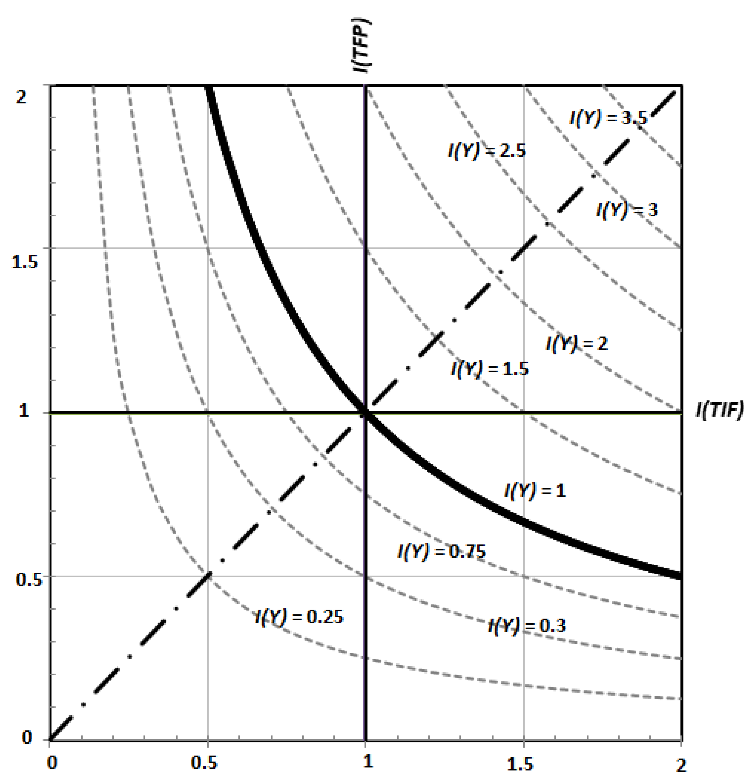
Equations (3) and (4), respectively, constitute a starting point to determine how the changing inputs (in our case represented by TIF), i.e., extensive factors, and the changing productivity (total factor productivity), i.e., intensive factors, contribute to the change of output (product). To be clear look at the Figure 2. In this figure, we plotted the isoquants for the system output index, i.e., I(Y)—these isoquants represent all values I(TFP) and I(TIF), which result in the same value I(Y). These hyperbolic isoquants can be expressed as
I(TFP) = I(Y)/I(TIF)
Equation (5) shows that the isoquants of constant system output development I(Y) are equilateral hyperbolas with variable curves and with constant elasticity equal to 1. The product stagnation hyperbola, which intersects the coordinate origin (1; 1), is of special importance. All isoquants above that hyperbola represent output growth—for instance, the isoquant with value 2 in Figure 2 illustrates all combinations of I(TIF) and I(TFP) that double the output. All isoquants below the output stagnation hyperbola represent a decrease in the system output.
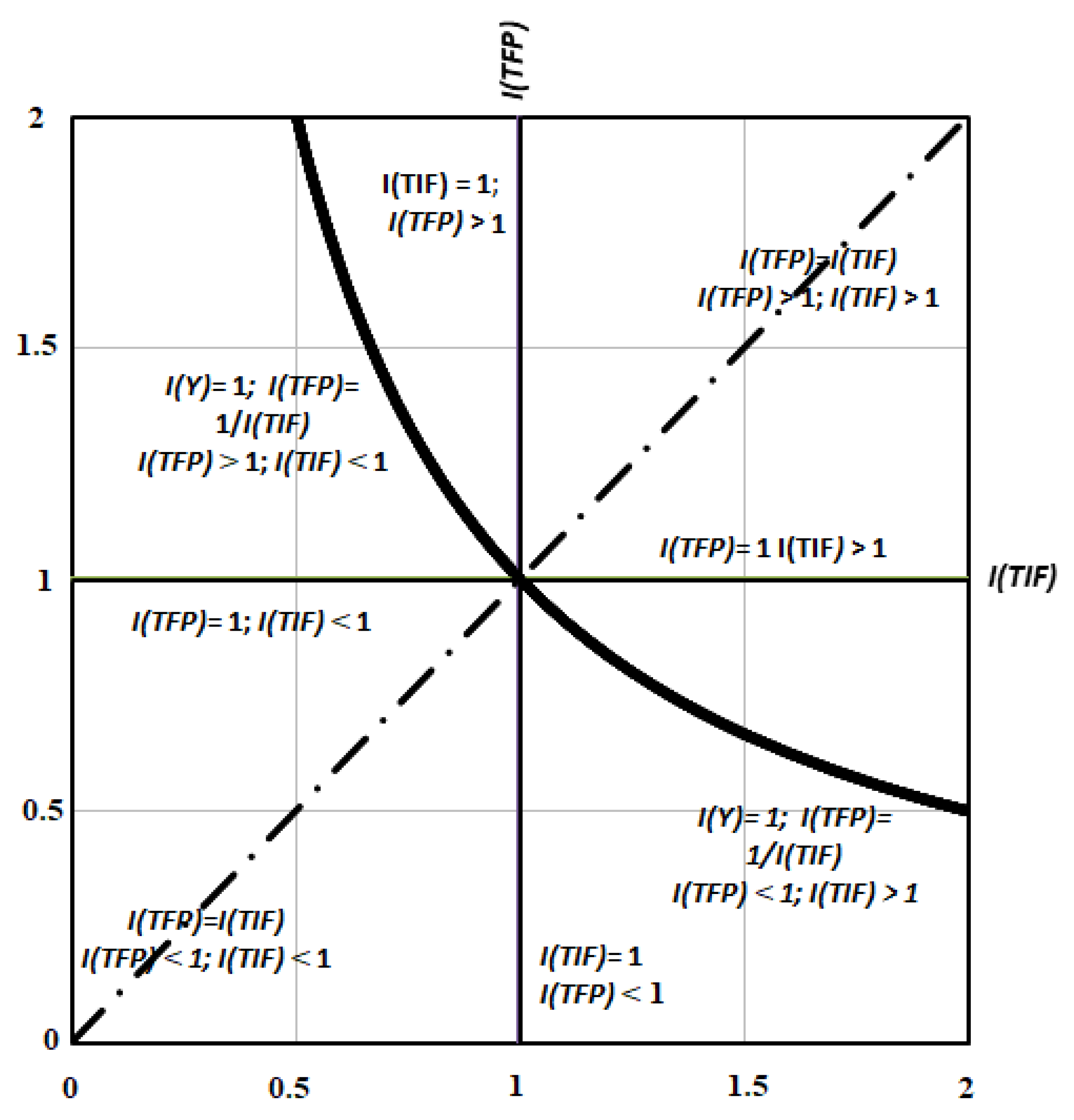
Figure 2 also indicates the basic types of relationships between the development of extensive and intensive factors on the one hand and the output development on the other hand. These basic types of relationships (basic development scenarios), which are precisely described in Figure 3 include the following:
- Pure developments, which are situated on coordinate axes of Figure 3. The product only grows or declines as a result of one of the factors under consideration, either purely extensively or purely intensively. The other one remains unchanged, i.e., I(TIF) = 1 (for a purely intensive change) or I(TFP) = 1 (for a purely extensive change). Pure developments can be further distinguished to pure growth and pure decline. Pure extensive growth (I(TIF) > 1 and I(TFP) = 1) is indicated by the positive ray of axis x, while pure extensive decline (I(TIF) < 1 and I(TFP) = 1) is indicated by the negative ray of axis x. Similarly: purely intensive growth (I(TFP) > 1 and I(TIF) = 1) is indicated by the positive ray of axis y, while purely intensive decline (I(TFP) < 1 and I(TIF) = 1) is indicated by the negative ray of axis y.
- Balanced developments. Both factors under consideration have the same effect, i.e., I(TIF) = I(TFP). In Figure 3, these developments are situated in quadrants I and III on a straight line at the angle of 45 degrees, which intersects the origin of coordinate axes. The developments can be further distinguished to intensive–extensive growth and intensive–extensive decline. The former is represented by the positive section of the straight line at the angle of 45 degrees, the later by negative section of this straight line.
- Compensatory developments. Both factors fully compensate each other into product stagnation, i.e., I(Y) = 1, and thus I(TFP) = 1/I(TIF). These developments lie on the hyperbolic isoquant of product stagnation (see above). The upper half of the hyperbola represents intensive–extensive compensation where I(TFP) > 1 and I(TIF) < 1. The lower half of hyperbola represents extensive–intensive compensation—where I(TFP) < 1 and I(TIF) > 1.
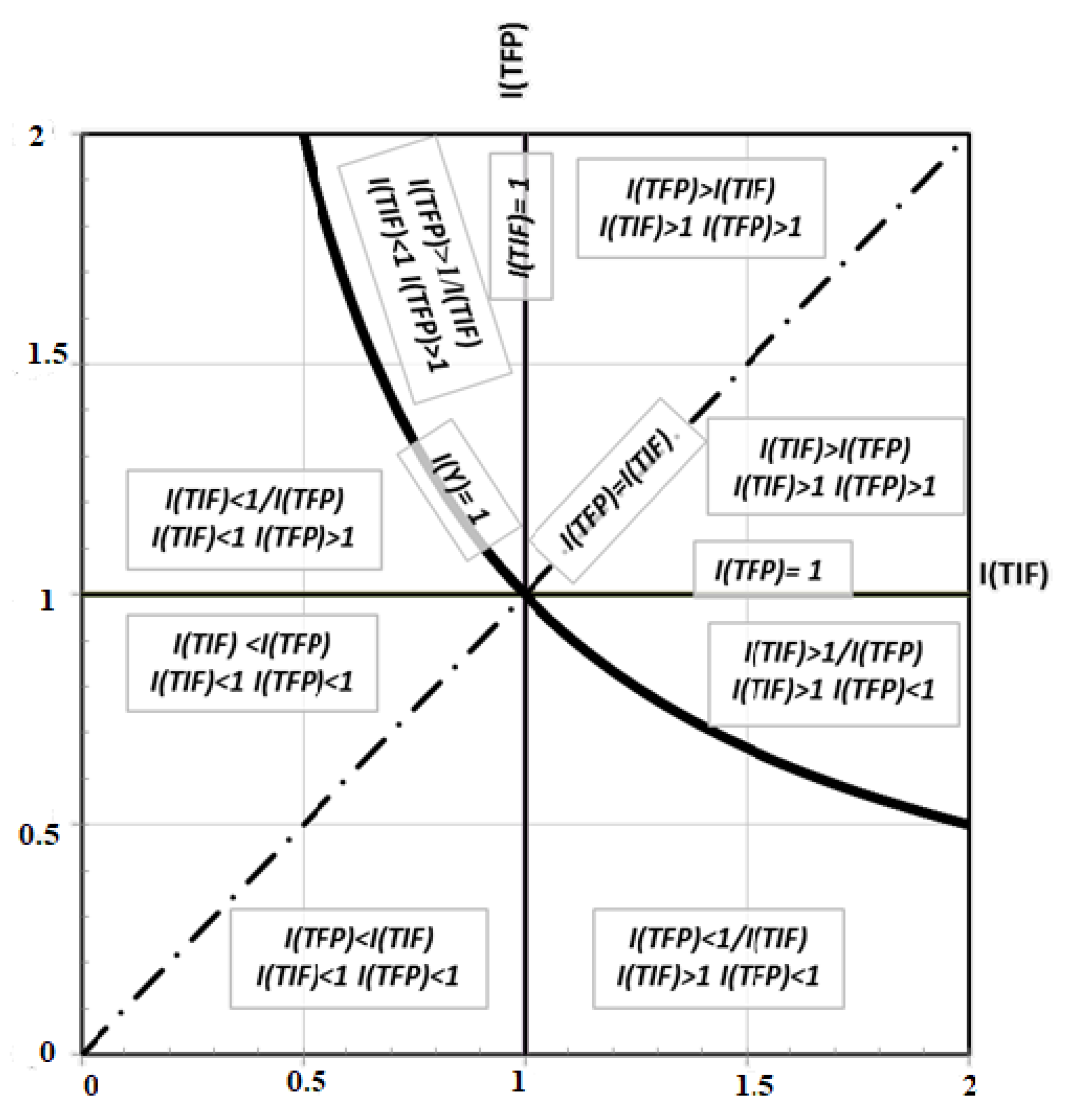
As already stated in the introduction, the basic types of developments are usually rare. It is not very likely that the system output would grow or decline purely intensively or purely extensively (i.e., slightly more likely indeed); that both factors (I(TIF) and I(TFP)) would have the same effect on system growth or decline; and the situation where the system does not change at all (I(Y) = 1) as a result of fully compensatory effects of both factors probably occurs rarely. Therefore, attention needs to be paid to combined types of development. This includes all the other situations. Graphically, in the charts concerned, such situations lie outside the coordinate axes, the 45-degree straight lines in quadrants I and III, intersecting the origin of the coordinate axes, as well as outside the hyperbolic stagnation isoquant. This applies to eight spaces, which can always be characterized by three inequations, which also determine whether or not the output grows, i.e., I(Y) > 1 or I(Y) < 1. The first of the three inequations determines the relationship between I(TFP) and I(TIF) or, for compensatory developments, between this quantity and an inverted value of the other. The second inequation determines whether the TIF rises or falls, i.e., I(TIF) > 1 or I(TIF) < 1. The third inequation determines whether the TFP rises or falls, i.e., I(TFP) > 1 or I(TFP) < 1. Thus, for example, the space in which I(Y) > 1 and at the same time I(TFP) > 1/I(TIF), with I(TFP) > 1 and I(TIF) < 1, represents combined developments shown in the plane between the positive direction of axis y and the upper section of the stagnation hyperbola. With these developments, the product grows although the TIF declines. This means that the rise in TFP not only compensates the decline in TIF but also causes the product to grow. The relationships between I(TFP) and I(TIF) for all basic and combined types of developments are plotted in Figure 4 and Table 1.
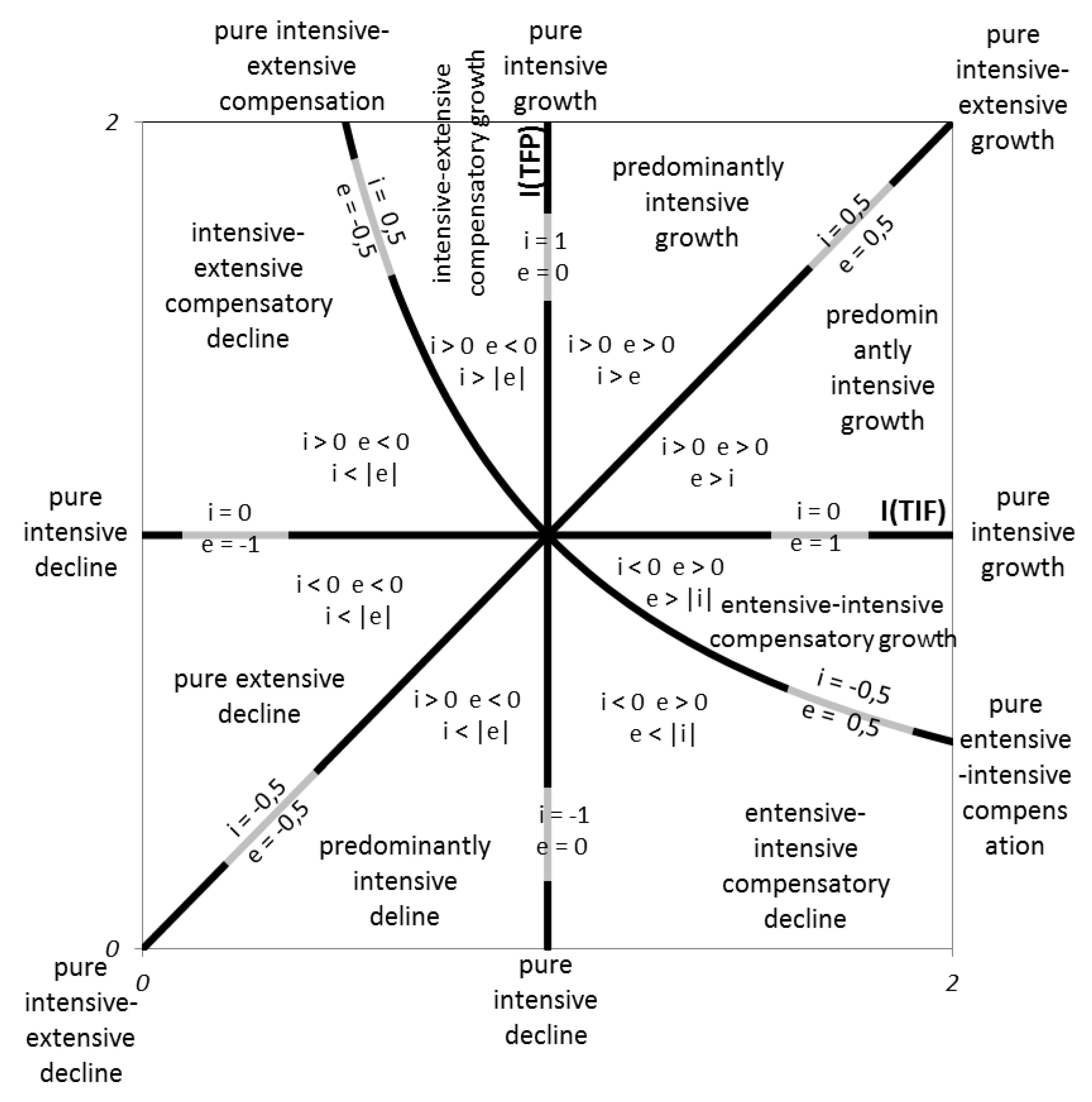
It would be worth assigning such names to the individual spaces shown in Figure 4 that, if possible, most accurately express what happens in reality. Therefore, we are presenting a comprehensive nomenclature of all basic and combined developments. We follow the following six principles, which we consistently apply below:
- The nomenclature must cover all types of developments.
- If the system product (output) grows, we use the word “growth”; if it declines, we use the word “decline”; if it remains unchanged, we use the words “pure compensation”.
- We refer to all basic developments as “pure”.
- When referring to consonant developments, i.e., those where both factors drive growth or both factors drive decline in system output, but they do so unequally, we use the word “predominantly”, and use the name of the predominant factor. This means that predominantly intensive growth indicates the situation where both factors (I(TIF) and I(TFP)) drive growth, but the impact of intensive factors is greater than that of extensive factors. Likewise, predominantly extensive decline depicts the situation where both factors (I(TIF) and I(TFP)) drive decline, but the impact of extensive factors is greater than that of intensive factors.
- When referring to dissonant developments, i.e., those where one factor drives growth and the other drives decline in system output, we use the word “compensation” or “compensatory”.
- If the names of combined compensatory or purely compensatory developments concurrently include the words “intensive” and “extensive”, we use—as the first of the words intensive and extensive—the one which drives growth, followed by the one that drives decline. For instance, the term intensive–extensive compensatory growth refers to the situation where the intensive factors grow so rapidly that they partly compensate a decline in the extensive factors, thus making the system grow in the end (see the situation above, where I(Y) > 1 and at the same time I(TFP) > 1/I(TIF)), with I(TIF) < 1 and at the same time I(TFP) > 1. Likewise, an intensive–extensive compensatory decline indicates the situation where the intensive factors grow while the extensive factors decline, making system output decline in the end. In this logic, a pure intensive–extensive compensation shows the situation where the intensive factors drive growth and the extensive factors concurrently drive decline, making the system output stagnate in the end (a pure extensive–intensive compensation defines the opposite situation, where the extensive factors drive growth, the intensive factors drive decline, making system output stagnate again).
3. Dynamic Parameters of Intensity and Extensity
For now, we described all the possible ways how a change in the intensive factors, a change in the extensive factors or their combination affect the change in product. However, we have not yet quantified the impact of the changes in intensive or extensive factors on that change. The so-called dynamic parameters of intensity and extensity are used for this quantification. These can be derived from expression (3). The expression must first be logarithmised. We obtain
ln I(Y) = ln I(TFP) + ln I(TIF)
The parameters are designed to ensure that their values correspond to the development typology we derived above. Specifically, if a change of any factor contributes to production growth, the relevant parameter should be positive (e.g., if a change of intensive factors contributes to growth, the dynamic parameter of intensity is positive), whereas if it leads to a decline in output, the parameter value is negative. If the given factor remains unchanged, the relevant parameter is equal to zero. The values of the parameters are between −1 and 1. The following applies to the sum of absolute values of relevant parameters
Therefore, the parameters express how much, in % (after multiplying by 100), the intensive or extensive factors contribute to the output growth or decline. For instance, if dynamic parameter of intensity has value 0.6 and dynamic parameter of extensity has value 0.4 it means the former contributes to growth of a system output by 60% and the later by 40%.
In order to achieve the above mentioned, when expressing the share of ln I(TFP) or ln I(TIF) in the total value (sum of ln I(TFP) + ln I(TIF)), we need to adjust the denominator and work with absolute values, with expressions |ln I(TFP)| a |ln I(TIF)| The dynamic parameter of intensity showing the share of impact of change in the intensive factors (I(TFP)) for all of the development types referred to above is
An analogical dynamic parameter of extensity expresses the share of the impact of extensive factors (I(TIF)) for all types of developments
More details concerning the parameters are available in [11,12]. The assignment of both parameters’ values to individual developments is specified in Table 1, where names according to the above mentioned nomenclature are also assigned to the respective situations.
The following should apply for the successful economic system (i.e., the system achieving to satisfy more needs): their output and consequently their difference between outputs and inputs are increasing over time, while this growth is caused mainly by intensive factors. In general, an economic system should aim at ensuring a positive parameter of intensity, while maximizing its value in the long run. We understand that, in many areas, crucial innovations have already been realized a long time ago, and current innovations are only marginal compared to such crucial ones; consequently, the dynamic parameter of intensity cannot come near the value of 1 in the case of a successful system, where production (output) are increasing. However, it is still true that this parameter should be positive. A negative value of this parameter in the long term (for three years or more) signals that the system is in difficulty.
Our classification demonstrates that a system’s performance may be positive and increasing even though the value of parameter i is negative. This situation is shown in row 6 of Table 1 and we called it extensive and de-intensive growth—the decline in intensive factors is offset by an increase in extensive factors. Similarly, the situation shown in row 8 is also dangerous, as intensive factors are declining, but extensive factors are increasing at the same rate, thereby offsetting the decline in intensive factors. In this case, the system’s output does not change. This may cause the management of the system to become complacent, believing that everything is in order. Neither extensive and de-intensive growth, nor extensive offsetting, are sustainable on a long-term basis. Sooner or later, the system will hit the input barrier and be unable to outweigh or offset the decline in intensive factors, a situation which may even result in its dissolution. Other situations described in Table 1 may also be alarming, such as the situation in row 1 with an increase only in extensive factors only or the situation in row 4, especially if the value of dynamic extensity parameter is in long term much higher rate than the value of dynamic intensity parameter. These situations represent a risk that the system will, sooner or later, also hit the barrier to further expansion of inputs—i.e., it will not be able to generate further growth in the existing manner.
A decline in intensive factors (a negative dynamic intensity parameter) is a signal that output may fall. Row 11 of Table 1 shows the situation where the growth in extensive factors cannot offset the decline in intensive factors, rows 12 and 14 show a decline in both intensive and extensive factors, while row 15 describes a decline in extensive factors and no change in intensive factors. All these situations adversely affect the system’s output. A system should pay the attention to all above mentioned dangerous or alarming situations and try such steps increasing the value of the dynamic intensity parameter. It must be emphasized that if the system is a company standard, methods of its evaluation as financial analysis (e.g., [1]) need not reveal that the company does not develop intensively (for details see [9]). Therefore, the parameters should be used as the additional source for company analysis.
4. Comparison Our Approach with Other Methods to Quantify Impact Intensive and Extensive Factors
As mentioned in the introduction, one of the most important attempts to quantify the impact of intense and extensive factors is growth accounting equation. It counts how growth rate of labor, growth rate of capital (both growth rates represent extensive factors), and growth rate of TFP (an intensive factor) contribute to growth rate of GDP. The key methodical difference between our methodology and growth accounting is that dynamic parameters are based on a simple multiplicative link (1) and at the next level on the weighted multiplicative link of labor and capital indices (2), whereas the primary approach to growth accounting (e.g., [5,20,23,25,26,27,28] is based on the additive weighted aggregation of labor and capital).
where MPPk is the marginal product of capital and MPPl is the marginal product of labor.
Y = MPPk K + MPPl L
The methodology of growth accounting is not reasonably able to quantify situations when either GDP or labor or capital decline or stagnate. Generally, it does not work with complex typologies of all types of developments. It can be further discussed (e.g., [17,29,30]) whether it is possible to separate the inputs on labor and capital without biasing the results, as usually no factor alone can contribute to output and its change.
If analysts (e.g., [31,32]) using growth accounting want to express the share in the impact of intensive factors if, they divide the TFP growth rate by the rate of GDP growth G(Y). For the share of the impact of intensive factors, we will thus obtain the expression
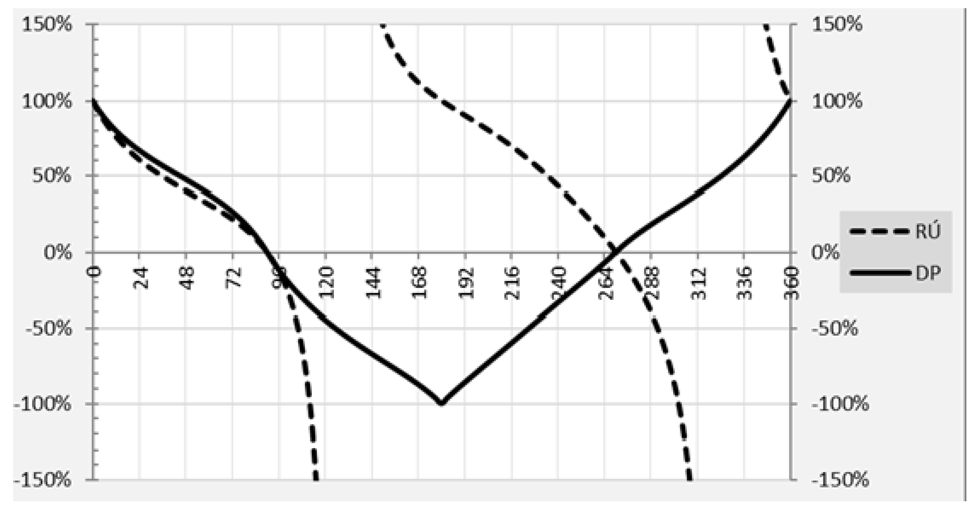
A disadvantage of expression (11) is that its values are not always meaningful for all possible types of development. Expressed in percentages, expression (11) delivers values of −∞ to +∞. With our presented methodology (i.e., the dynamic parameter of intensity), the values according to expression (11) are only consistent for purely intensive growth and purely extensive growth or approximately for very small positive growth rates within 1%. Much the same results would also be obtained for quadrant I, where growth takes place because of both considered factors. In quadrants other than I [0 to 90°], the values of expression (11) and of the dynamic parameter of intensity differ greatly. For purely intensive–extensive growth or decline (i.e., where both TFP and TIF equally grow or decline), expression (11) delivers values different from 50%, with the deviation rising with the rising rate (see Appendix Table A1). In addition, where one factor drives growth and the other equally drives decline, expression (11) delivers different results for the individual rates of growth or decline (see Appendix Table A2). Dynamic parameters of intensity and extensity describe the impact of TIF and TFP change more clearly than growth accounting. Therefore, the parameters can be an appropriate addition or alternative to growth accounting. Basic comparison the values of dynamic parameters with expression (11) is made in the Figure 6.
5. Results
To demonstrate the capability of the parameters, we use them from the macroeconomic point of view (it means for the macroeconomic systems) and calculated them for German and Czech GDP development for the period 1991–2017. The task was to find how intensive and extensive factors contribute to GDP development of both countries. The input data for the calculation—data of the input (G(K) and G(L)) development and data of output development ((G(Y))—was for both countries taken or count from [33,34]. The data for the year 2017 are preliminary. G(Y) and G(K) is expressed in in constant prices of the year 2010. The algorithm for the calculations shown below is the same for both analyzed countries.
- Using the three initial growth rates, we calculate the average growth rate for the entire period.
- We calculate the growth rate of capital labour equipment G(K/L) using the equation
- We calculate the growth rate of the aggregate input factor G(TIF) using the equation
- We calculate the growth rate of aggregate productivity G(TFP) using the equation
- The dynamic parameters of intensity and extensity and dynamic parameters of the share of the influence of the labor or capital development on the TIF development are calculated according to Equations (8) and (9).
All input data (G(Y), G(K), G(L)) and calculated results (G(K/L), G(TIF), G(TFP), i, e, k, l) are summarized in percentage form in Table 2 for Germany and in Table 3 for the Czech Republic.
The very similar economic development in Germany and the Czech Republic (CZ) is clear from Figure 7 describing GDP development in both countries at constant 2010 prices. This similarity is due to numerous interrelations between the two economies, which also has historical roots. Deviations are more essential in the 1990s, when the CZ was going through economic transformations including economic crisis at the second half of the period and Germany had to solve the consequences of the reunification in 1990. The CZ has higher growth rate period after the year 2000 as the consequence of its preparation on EU membership. The EU entrance was connected with capital inflow that brought to the country new modern technology. It also meant higher international involvement and cooperation, higher international division of labor and other positive factors. The result was a quite high Czech growth rate and high positive yearly values of dynamic intensity parameter. Both countries were hit by the deep crisis in 2009. The recovery from the crisis after 2009 also happens similarly.
As shown in the last lines of Table 2 and Table 3, the CZ achieved an only slightly higher average GDP growth rate for the whole period, i.e., 1.77% compared to 1.47% for Germany. The biggest difference is in the labor factor, which in the CZ is declining on average by a quarter of a percent year-on-year, while in Germany it is growing by half-a-percent. Intensity and extensity are also very similar, since in both cases there is predominantly extensive development, however with high intensity. The intensity in the CZ is 4 percentage points higher, reaching 42%, while in Germany it is 38%. The balance up to 100% in both countries is extensive development.
If we concentrate on the columns i and e in the Table 2 and Table 3, it is possible to see the year-on-year development in intensity and extensity is similar in both countries, especially after the period of transformation in the 1990s. The processes of transformation of the Czech economy and the impacts of German unification were nevertheless different in nature. Former East Germany can rely on wealthy West Germany that can easily export to East Germany its technology, knowledge, and other factors. People form East Germany could further move to west and to find here jobs that was connected with higher level of capital goods that increased their productivity. All these factors caused mainly positive values of dynamic intensity parameter (i). The position of the CZ was more difficult. Czech economic transformation meant deeper changes resulting in negative values of dynamic intensity parameter in the beginning of the transformation. Negative German values of dynamic intensity parameters in years 1998 and 1999 were mainly due to the entry of Germany into the euro area. Entry into the euro area is a process in which we can expect negative extensity.
The period 2000–2007 means positive values of dynamic intensity parameter for both countries in whole period (except year 2006 in the case of Germany and 2007 in the case of the CZ). Germany was able to succeed in liberalization of labor market (so called The Hartz Reform, see e.g., [35] for details). It also uses the fact that euro exchange rate is generally under-valuated in its case what is favorable for German export. The more intensive development in the CZ in the same period can be attributed to the preparation of the CZ for accession to the EU and the impacts of this serious step.
The crisis in year 2009 brought negative values of both parameters in the case of the CZ and negative value of German dynamic extensity parameter. The process of recovery from the crisis are connected with slightly different Czech and German values of both parameter. However, the values of parameters are affected by temporary demand shock and interpretation of their year values can be misleading (see Chapter 6 for details). When we shortly move to the to the analysis of the dynamic parameter of the share of the influence of the labor development on the development of TIF (l) and the dynamic parameter of the share of the influence of the capital development on the development of TIF (k) we find higher differences. They are due to different labor mobility (generally higher in Germany) and higher change of capital structure that was realized in the CZ and other factors.
6. Discussion
How accurate are the dynamic intensity and extensity parameters? And do they always describe exactly what happens in reality? The values of the parameters depend, of course, on input data. Our approach uses as the input data only growth rates of labor, capital, and GDP. The analysis looks at labor and capital as a homogeneous factor and it does not consider other features as education, skill, quality of capital goods, and so on. However, identical value of labor or capital change can result in different GDP development. For instance, if one country experiences growth of educated labor force (e.g., people with university education) and the second on growth of unskilled person. Although labor growth rates are equal in both countries GDP growth rates differ. Similarly, if one country is introducing modern technically-progressive capital goods and the second one increases number of obsolete ones, the change of GDP will be probably different even in the case when both changes of capital are expressed by same value. It is reasonable to expect that the change containing a qualitative character will result in higher TFP change of and thus in higher value of dynamic intensity parameter.
If we want to distinguish quality of inputs, it is possible to add to equation other factors or to divide labor and capital to more specific forms. Equation (3) then can be rewritten e.g. as
where i and j represents different forms of capital and labor.
The Equation (5) can then be rewritten as
Share of the influence of the specific factor (e.g., educated labor force) on TIF development can be then expressed as
The other possible disadvantage of the parameters is that interpretation of their values can be sometimes misleading. Especially in the case of sudden demand or supply shocks. Yearly values of both parameters are usually affected by a shock. For instance, the output in the case of negative demand shock decreases, but amount of inputs usually does not decrease in the same rate. The input decline is usually lower, or inputs can even stagnate or grow especially in the beginning of the shock when their development is not affected by the shock. The dynamic parameter of intensity is negative in such case. However, the country does not experience real technological regression. It is reasonable for firms not to reduce the amount of inputs in same rate as output decline. If the negative shock is temporary, it makes sense to keep the inputs in the firms and to avoid costs connected with input reduction and subsequent input increase. Oppositely, when the demand shock ends, inputs and output usually grow but the input change is lower that the output change. The value of dynamic intensity parameter is positive, but it does not mean real technological progress. Firms only started to use more inputs that had not been reduced during shock.
Negative supply shock due to sudden increase prices of inputs (e.g., oil) can cause misinterpretation too. The change of inputs is usually higher than change of output due to the shock. Value of inputs usually grows; value of output grows smaller, stagnates, or even declines. The result is negative value of dynamic intensity parameter which, however, does not again mean technological regression. The economy is not only able to respond appropriately in the short run to the shock. Generally, yearly values of dynamic intensity and extensity parameters express what happens on the aggregate level. Their negative values can be seen as a sign of some economic problems, but the essence of the problem must be further investigated. It is not possible to conclude without other research that yearly negative values mean real technological regression or real decline of inputs. Yearly negative value of dynamic extensive parameters can be further caused by change of depreciation methodology or by the fact the new capital good cost less than the removed ones.
Extraordinary yearly positive values of both parameters must be carefully analyzed too as they often describe the situation when an economy improves from previous negative development. The positive values thus balance what happened in the past. The value of the parameters can be also misleading in the case when all values (I(TIF), I(TFP), I(Y)) are close to 1—so they describe slight change. The small difference in their values in such situation can cause extraordinary value of any dynamic parameter—e.g., value of i is 98% and value of e is 2%. A big technological change seems to happen, but it does not. Long run values of both parameters counted e.g., for a 10-year period describe technological progress or regression more preciously. Long run development is not affected by temporary shocks, it contains higher aggregate values of I(TIF), I(TFP), and I(Y) and it is possible to analyze whether GDP development is really based on intensive or extensive factors.
It must be further emphasized that the logic of the parameters is based on the presented model. Its key relationship is the Equation (1) seeing system output as the product of system inputs and system productivity. It is, of course, questionable whether output can be expressed in this simple expression. Even if we use some weighted expression to calculate productivity (such expression can be derived e.g., from Equation (15)), it can still be argued that there is no linear relationship between inputs and outputs and that such relationship is more complex or complicated. Although our model is in accordance with mainstream scientific literature (see Section 2 for details) it is true that change of system output can be also caused by other factors that are not including in inputs and their productivity and thus cannot be assigned to the extensive or intensive change. A possible solution of the problem is offered in [21]—to see productivity change in a broad sense as any change causing any shift in production function. What caused the shift must be then carefully investigated before the real nature of the change is determined.
7. Conclusions
The article presents a complex typology of relationships between the development of total factor productivity (TFP) and total input factor (TIF) of any system on the one hand and output development on the other. This typology is based on a multiplicative link, where the output is defined as the product of TFP times TIF. The typology includes, inter alia, pure developments, where the output changes either only as a result of a TFP change or a TIF change, or the change of TFP is equal to TIF, i.e., with both factors equally counteracting each other, resulting in output stagnation. In addition, the article describes all mixed developments which make the output change (grow or decline) as a result of a current (growing or declining) change in TFP and TIF. This typology is used as the basis of the proposed dynamic parameters of intensity and extensity. These quantify the percentage share of the impact of intensive factors (I(TFP)) and extensive factors (I(TIF)) in output change. The values of these parameters range from −100% to 100% and are easy to interpret. The universality of our concept is compared to growth accounting, which does not separate the measurements of development intensity from the problem of substitution of technology for labor; explicitly, it does not address the problem of expressing intensive and extensive impacts, and is not sufficiently accurate for higher growth rates (over approximately 5%). Moreover, matters are complicated by the necessity of working with the weights of the impacts of growth sub-factors. In growth accounting, the expression of the shares of impacts of individual factors in output (GDP) change as a share of rates of growth G(TFP) or G(TIF) and G(Y) is also problematic, as these shares are not standardized into an easily interpretable interval, with their values ranging from −∞% to ∞%. Our methodology including dynamic parameters offers a logical indisputable system of all relationships between I(TFP), I(TIF), and I(Y), and assigns each situation a clear and meaningful title and values for both parameters. It can thus be seen as a possible alternative to growth accounting.
The calculations of the parameters for the development of Czech and German economy in the period 1991–2017 shows that the parameters give meaningful results that clearly depict the key events in the development of both countries. The values of parameters confirm similar economic development and the dependence of Czech economy on Germany. Larger differences are apparent in all the monitored characteristics in the 1990s, which were a period of fundamental transformation in the CZ, while Germany was dealing with the consequences of unification. The beginning of the millennium in Germany was mainly influenced by its entry into the euro area, while the CZ subsequently acceded to the EU. The pre-crisis period and the recovery from the crisis were very similar in both countries. The slightly higher intensity in the CZ for whole period 1991–2017 comes mainly from the convergence process.
Author Contributions
J.M. and P.W. developed complex nomenclature of all possible relationships among total input factor of an economic system, their productivity, and system output including names of all situation. They also developed dynamic intensity and extensity parameters, assigned their value to the presented nomenclature, and they discussed which values of parameters an economic system should achieve in long run. J.M. and J.K. counted values of the parameters for development of Czech and German GDP. J.K. and P.W. discussed advantages and shortages of the parameters.
Acknowledgments
The paper was created during solution the student project “Zdokonalení penzijního systému jako intenzifikační faktor ekonomiky” (“Improving pension system as one of the intensive economic factors”) that uses purpose-built support for specific university research of University of Finance and Administration.
Conflicts of Interest
The authors declare no conflict of interest.
Appendix A

Table A1.
Different values of Equation (11) and the dynamic parameter of intensity for purely intensive–extensive growth or decline (in %). Source: authors.
Table A1.
Different values of Equation (11) and the dynamic parameter of intensity for purely intensive–extensive growth or decline (in %). Source: authors.
| Purely Intensive–Extensive Growth | Purely Intensive–Extensive Decline | ||||||||
|---|---|---|---|---|---|---|---|---|---|
| G(SPF) | G(SIF) | G(Y) | if | i | G(SPF) | G(SIF) | G(Y) | if | i |
| 1 | 1 | 2 | 50 | 50 | −1 | −1 | −2 | 50 | −50 |
| 5 | 5 | 10 | 49 | 50 | −5 | −5 | −10 | 51 | −50 |
| 10 | 10 | 21 | 48 | 50 | −10 | −10 | −19 | 53 | −50 |
| 15 | 15 | 32 | 47 | 50 | −15 | −15 | −28 | 54 | −50 |
| 20 | 20 | 44 | 45 | 50 | −20 | −20 | −36 | 56 | −50 |
Table A2.
Different values of Equation (11) and the dynamic parameter of intensity for purely extensive–intensive compensation or purely intensive–extensive compensation (in %). Source: authors.
Table A2.
Different values of Equation (11) and the dynamic parameter of intensity for purely extensive–intensive compensation or purely intensive–extensive compensation (in %). Source: authors.
| Purely Extensive–Intensive Compensation | Purely Intensive–Extensive Compensation | ||||||||
|---|---|---|---|---|---|---|---|---|---|
| G(SPF) | G(SIF) | G(Y) | if | i | G(SPF) | G(SIF) | G(Y) | if | i |
| 1 | −1 | −0.01 | −10,000 | 50 | −1 | 1 | −0.01 | 10,000 | −50 |
| 5 | −5 | −0.25 | −2000 | 50 | −5 | 5 | −0.25 | 2000 | −50 |
| 10 | −10 | −1.00 | −1000 | 50 | −10 | 10 | −1.00 | 1000 | −50 |
| 15 | −15 | −2.25 | −667 | 50 | −15 | 15 | −2.25 | 667 | −50 |
| 20 | −20 | −4.00 | −500 | 50 | −20 | 20 | −4.00 | 500 | −50 |
References
- Froeb, L.M.; Ward, M. R: Managerial Economics, 4th ed.; Cengage Learning: London, UK, 2015. [Google Scholar]
- Mankiw, N.G. Principles of Economics; South-Western College Pub.: Nashville, TN, USA, 2017. [Google Scholar]
- Sandamo, A. Economic Evolving; Princeton University Press: Princeton, NJ, USA, 2011. [Google Scholar]
- Barro, R. Notes on Growth Accounting. J. Econ. Growth 1999, 2, 119–137. [Google Scholar] [CrossRef]
- La Grandville, O. Economic Growth: A Unified Approach; Cambridge University Press: Cambridge, UK, 2016. [Google Scholar]
- Romer, P. Endogenous Technological Change. J. Political Econ. 1990, 5, 71–102. [Google Scholar] [CrossRef]
- Cyhelský, L.; Mihola, J.; Wawrosz, P. Quality Indicators of Economic Development at All Level of the Economy. Statistika (Stat. Econ. J.) 2012, 2, 29–43. [Google Scholar]
- Hájek, M.; Mihola, J. Analýza vlivu souhrnné produktivity faktorů na ekonomický růst České republiky. Pol. Ekon. 2009, 6, 740–753. [Google Scholar]
- Kotěšovcová, J.; Mihola, J.; Wawrosz, P. Is the Most Innovative Firm in the World Really Innovative? Int. Adv. Econ. Res. 2015, 21, 41–54. [Google Scholar] [CrossRef]
- Kotěšovcová, J.; Mihola, J.; Wawrosz, P. The Complex Typology of the Relationship between GDP and Its Sources. Ekon. Čas. 2017, 10, 775–795. [Google Scholar]
- Mihola, J. Agregátní produkční funkce a podíl vlivu intenzivních faktorů. Statistika 2007, 2, 108–132. [Google Scholar]
- Mihola, J. Souhrnná produktivita faktorů—přímý výpočet. Statistika 2007, 6, 446–463. [Google Scholar]
- Mihola, J.; Wawrosz, P. Development Intensity of four Prominent Economies. Statistika (Stat. Econ. J.) 2013, 3, 26–40. [Google Scholar]
- Mihola, J.; Wawrosz, P. Alternativní metoda měření extenzivních a intenzivních faktorů změny HDP a její aplikace na HDP USA a Číny. Pol. Ekon. 2014, 5, 583–604. [Google Scholar] [CrossRef]
- Mihola, J.; Wawrosz, P. Analýza vývoje intenzity hrubého domácího produktu České republiky a Slovenské republiky. Ekon. Čas. 2015, 8, 775–795. [Google Scholar]
- Foster, L.; Haltiwanger, J.; Syverson, C. Reallocation, firm turnover and Efficiency: Selection on Productivity or Profitability? Am. Econ. Rev. 2008, 98, 394–425. [Google Scholar] [CrossRef]
- Čekmeová, P. Total Factor Productivity and its Determinants in the European Union. J. Int. Relationsh. (Bratislava) 2016, 1, 19–35. [Google Scholar]
- Hall, R.; Jones, C. Why some countries produce so much output per worker than others? Q. J. Econ. 1999, 114, 83–116. [Google Scholar] [CrossRef]
- Krugman, P. The Age of Diminishing Expectations. US Economic Policy in the 1990s; MIT Press: Cambridge, MA, USA, 1994. [Google Scholar]
- Solow, R.M. A Contribution to the Theory of Economic Growth. Q. J. Econ. 1956, 1, 65–94. [Google Scholar] [CrossRef]
- Solow, R.M. Technical Change and the Aggregate Production Function. Rev. Econ. Stat. 1957, 3, 312–320. [Google Scholar] [CrossRef]
- Swan, T.W. Economic Growth and Capital Accumulation. Econ. Rec. 1956, 2, 334–361. [Google Scholar] [CrossRef]
- Barro, R.; Sala-I-Martin, X. Economic Growth, 2nd ed.; MIT Press: Cambridge, MA, USA, 1999. [Google Scholar]
- Cobb, C.W.; Douglas, P.H. A Theory of Production. Am. Econ. Rev. 1928, 18, 139–165. [Google Scholar]
- Denison, E.F. The Source of Economic Growth in the United States and the Alternatives before Us; Committee for Economic Development: Washington, DC, USA, 1962. [Google Scholar]
- Jorgeson, D.; Griliches, Z. The explanation of productivity changes. Rev. Econ. Stud. 1967, 34, 249–280. [Google Scholar] [CrossRef]
- Kendrick, J.W. Productivity Trend in the United States; Princeton University Press: Princeton, NJ, USA, 1961. [Google Scholar]
- Gordon, R.J. The rise and fall of American growth. In The U.S. Standard Livening Since Civil War; Princeton University Press: Princeton, NJ, USA, 2016. [Google Scholar]
- Bisonyabut, N. Growth Accounting: Its Past, Present and Future. TDRI Q. Rev. 2012, 1, 12–18. [Google Scholar]
- Oulton, N. The Mystery of TFP. Int. Prod. Monit. 2016, 31, 68–87. [Google Scholar]
- Baran, K.A. The Determinants of Economic Growth in Hungary, Poland, Slovakia and the Czech Republic during the Years 1995–2010. Equilibrium 2013, 3, 7–26. [Google Scholar] [CrossRef]
- Helísek, M. Makroekonomie Základní kurs, 2nd ed.; Melandrium: Prague, Czech Republic, 2002. [Google Scholar]
- AMECO Database. Available online: https://ec.europa.eu/info/business-economy-euro/indicators-statistics/economic-databases/macro-economic-database-ameco/ameco-database_en (accessed on 25 June 2017).
- Statistical annex of European Economy, Spring 2017. Available online: https://ec.europa.eu/info/sites/info/files/statistical_annex_ee_spring_2017.pdf (accessed on 25 June 2017).
- Krebs, T.; Scheffel, M. Macroeconomic Evaluation of Labor Market Reform in Germany. IMF Econ. Rev. 2013, 4, 664–701. [Google Scholar] [CrossRef]
Figure 1.
System output as the product of system total input factor and system total factor productivity. Source: authors.
Figure 1.
System output as the product of system total input factor and system total factor productivity. Source: authors.

Figure 2.
Plot of the area for development typology of I(Y), I(TIF) and I(TFP. Source: authors. The scope of indices for both factors (I(TFP) and I(TIF)) is selected within the range of (0; 2) i.e., from the output decrease, through output stagnation, to output growth to a double.
Figure 2.
Plot of the area for development typology of I(Y), I(TIF) and I(TFP. Source: authors. The scope of indices for both factors (I(TFP) and I(TIF)) is selected within the range of (0; 2) i.e., from the output decrease, through output stagnation, to output growth to a double.

Figure 3.
Detailed description of basic types of development I(Y), I(TIF) and I(TFP). Source: authors.
Figure 3.
Detailed description of basic types of development I(Y), I(TIF) and I(TFP). Source: authors.

Figure 4.
Representation of basic and combined types of development I(Y), I(TIF), and I(TFP). Source: authors.
Figure 4.
Representation of basic and combined types of development I(Y), I(TIF), and I(TFP). Source: authors.

Figure 5.
The complex nomenclature of all basic and mixed relationships among I(Y), I(TIF), and I(TFP). Source: authors.
Figure 5.
The complex nomenclature of all basic and mixed relationships among I(Y), I(TIF), and I(TFP). Source: authors.

Figure 6.
Comparison of expressions of development intensity using expressions (5) and (11). Source: authors. RÚ = growth accounting values according to expression (11), DP = values of dynamic parameter of intensity according to expression (5). Quadrant assignments: 0 to 90: quadrant I (top right), 90 to 180: quadrant II (top left), 180 to 270: quadrant III (bottom left), 270 to 360: quadrant IV (bottom right).

Figure 7.
GDP development for the period 1991 to 2017 for Germany (DE) and the Czech Republic (CZ). Source: [34,35]; authors.

Table 1.
Overview of individual types of development I(TIF) and I(TFP) and values of dynamic parameters of intensity and extensity. Source: authors.
Table 1.
Overview of individual types of development I(TIF) and I(TFP) and values of dynamic parameters of intensity and extensity. Source: authors.
| Change of Extensive Factors (I(TIF)) | Change of Intensive Factors (I(TFP)) | Change of Output (I(Y)) | Values of Intensity (i) and Extensity (e) | Type of Development | |
|---|---|---|---|---|---|
| 11 | growth, (I(TIF) > 1) | unchanged, (I(TFP) = 1) | growth, (I(Y) > 1) | e = 1; i = 0 | pure extensive growth |
| 22 | unchanged, (I(TIF) = 1) | growth, (I(TFP) > 1) | growth, (I(Y) > 1) | e = 0; i = 1 | pure intensive growth |
| 33 | same growth as intensive ones, (I(TIF) > 1, I(TIF) = I(TFP)) | same growth as extensive ones, (I(TFP) > 1, I(TFP) = I(TIF)) | growth, (I(Y) > 1) | e = 0.5; i = 0.5 | pure intensive–extensive growth |
| 44 | faster growth than intensive ones, (I(TIF) > 1, I(TIF) > I(TFP)) | slower growth than extensive ones, (I(TFP) > 1, I(TFP) < I(TIF)) | growth, (I(Y) > 1) | e > 0; i > 0; e > i | predominantly extensive growth |
| 55 | slower growth than intensive ones, (I(TIF) > 1, I(TIF) < I(TFP)) | faster growth than extensive ones, (I(TFP) > 1, I(TFP) > I(TIF)) | growth, (I(Y) > 1) | e > 0; i > 0; i > e | predominantly intensive growth |
| 66 | is greater than inverted value of intensive ones, (I(TIF) > 1, I(TIF) > 1/I(TFP)) | is greater than inverted value of extensive ones, (I(TFP) < 1, I(TFP) > 1/I(TIF)) | growth, (I(Y) > 1) | e > 0; i < 0; e > |i| | extensive–intensive compensatory growth |
| 77 | is greater than inverted value of intensive ones, (I(TIF) < 1, I(TIF) > 1/I(TFP)) | is greater than inverted value of extensive ones, (I(TFP) > 1, I(TFP) > 1/I(TIF)) | growth, (I(Y) > 1) | e <0; i> 0; i > |e| | intensive–extensive compensatory growth |
| 88 | equal to inverted value of intensive ones, (I(TIF) > 1, I(TIF) = 1/I(TFP)) | equal to inverted value of extensive ones, (I(TFP) < 1, I(TFP) = 1/I(TIF)) | no change (stagnation), (I(Y) = 1) | e = 0.5; i = −0.5 | pure extensive–intensive compensation |
| 99 | equal to inverted value of intensive ones, (I(TIF) < 1, I(TIF) = 1/I(TFP)) | equal to inverted value of extensive ones, (I(TFP) > 1, I(TFP) = 1/I(TIF)) | no change (stagnation), (I(Y) = 1) | e = −0.5; i = 0.5 | pure intensive–extensive compensation |
| 110 | is less than inverted value of intensive ones, (I(TIF) < 1, I(TIF) < 1/I(TFP)) | is less than inverted value of extensive ones, (I(TFP) > 1, I(TFP) < 1/I(TIF)) | decline, (I(Y) < 1) | e < 0; i > 0; i < |e| | intensive–extensive compensatory decline |
| 111 | is less than inverted value of intensive ones, (I(TIF) > 1, I(TIF) < 1/I(TFP)) | is less than inverted value of extensive ones, (I(TFP) < 1, I(TFP) < 1/I(TIF)) | decline, (I(Y) < 1) | e > 0; i < 0; e < |i| | extensive–intensive compensatory decline |
| 112 | faster decline than intensive ones, (I(TIF) < 1, I(TIF) < I(TFP)) | slower decline than extensive ones, (I(TFP) < 1, I(TFP) > I(TIF)) | decline, (I(Y) < 1) | e < 0; i < 0; |e| > |i| | predominantly extensive decline |
| 113 | slower decline than intensive ones, (I(TIF) < 1, I(TIF) > I(TFP)) | faster decline than extensive ones, (I(TFP) < 1, I(TFP) < I(TIF)) | decline, (I(Y) < 1) | e < 0; i < 0; |i| > |e| | predominantly intensive decline |
| 114 | same decline as intensive ones, (I(TIF) < 1, I(TIF) = I(TFP)) | same decline as extensive ones, (I(TFP) < 1, I(TFP) = I(TIF)) | decline, (I(Y) < 1) | e = −0.5; i = −0.5 | pure intensive–extensive decline |
| 115 | declining, (I(TIF) < 1) | unchanged, (I(TFP) = 1) | decline, (I(Y) < 1) | e = −1; i = 0 | pure extensive decline |
| 116 | unchanged, (I(TIF) = 1) | declining, (I(TFP) < 1) | decline, (I(Y) < 1) | e = 0; i = −1 | pure intensive decline |
Table 2.
Values of dynamic intensity and extensity parameters and dynamic parameters of the share of the influence of the labor or capital development on the development of TIF for Germany. Source: [33,34]; authors.
| Year | G(Y) | G(L) | G(K) | G(K/L) | G(TIF) | G(TFP) | Intensity i | Extensity e | Share l | Share k |
|---|---|---|---|---|---|---|---|---|---|---|
| 1991 | 5.1 | 2.8 | 5.3 | 2.4 | 4.0 | 1.0 | 20 | 80 | 35 | 65 |
| 1992 | 1.9 | −1.3 | 4.1 | 5.5 | 1.4 | 0.5 | 28 | 72 | −25 | 75 |
| 1993 | −1 | −1.3 | −4.2 | −2.9 | −2.8 | 1.8 | 39 | −61 | −23 | −77 |
| 1994 | 2.5 | 0 | 3.6 | 3.6 | 1.8 | 0.7 | 28 | 72 | 0 | 100 |
| 1995 | 1.7 | 0.4 | 0 | −0.4 | 0.2 | 1.5 | 88 | 12 | 100 | 0 |
| 1996 | 0.8 | 0 | −0.5 | −0.5 | −0.3 | 1.1 | 81 | −19 | 0 | −100 |
| 1997 | 1.8 | −0.1 | 0.8 | 0.9 | 0.3 | 1.4 | 80 | 20 | −11 | 89 |
| 1998 | 2 | 1.2 | 3.9 | 2.7 | 2.5 | −0.5 | −17 | 83 | 24 | 76 |
| 1999 | 2 | 1.6 | 4.6 | 3.0 | 3.1 | −1.1 | −26 | 74 | 26 | 74 |
| 2000 | 3 | 2.3 | 2.3 | 0.0 | 2.3 | 0.7 | 23 | 77 | 50 | 50 |
| 2001 | 1.7 | −0.3 | −2.5 | −2.2 | −1.4 | 3.2 | 69 | −31 | −11 | −89 |
| 2002 | 0 | −0.4 | −5.8 | −5.4 | −3.1 | 3.2 | 50 | −50 | −6 | −94 |
| 2003 | −0.7 | −1.1 | −1.3 | −0.2 | −1.2 | 0.5 | 29 | −71 | −46 | −54 |
| 2004 | 1.2 | 0.3 | 0 | −0.3 | 0.1 | 1.0 | 87 | 13 | 100 | 0 |
| 2005 | 0.7 | 0 | 0.7 | 0.7 | 0.3 | 0.3 | 50 | 50 | 0 | 100 |
| 2006 | 3.7 | 0.8 | 7.5 | 6.6 | 4.1 | −0.4 | −9 | 91 | 10 | 90 |
| 2007 | 3.3 | 1.7 | 4.1 | 2.4 | 2.9 | 0.4 | 12 | 88 | 30 | 70 |
| 2008 | 1.1 | 1.3 | 1.5 | 0.2 | 1.4 | −0.3 | −18 | 82 | 46 | 54 |
| 2009 | −5.6 | 0.1 | −10.1 | −10.2 | −5.1 | −0.5 | −8 | −92 | 1 | −99 |
| 2010 | 4.1 | 0.3 | 5.4 | 5.1 | 2.8 | 1.2 | 31 | 69 | 5 | 95 |
| 2011 | 3.7 | 1.4 | 7.2 | 5.7 | 4.3 | −0.5 | −11 | 89 | 17 | 83 |
| 2012 | 0.4 | 1.2 | −0.4 | −1.6 | 0.4 | 0.0 | 1 | 99 | 75 | −25 |
| 2013 | 0.3 | 0.6 | −1.3 | −1.9 | −0.4 | 0.7 | 65 | −35 | 31 | −69 |
| 2014 | 1.6 | 0.9 | 3.5 | 2.6 | 2.2 | −0.6 | −21 | 79 | 21 | 79 |
| 2015 | 1.7 | 0.8 | 2.2 | 1.4 | 1.5 | 0.2 | 12 | 88 | 27 | 73 |
| 2016 | 1.6 | 1.1 | 2.5 | 1.4 | 1.8 | −0.2 | −10 | 90 | 31 | 69 |
| 2017 | 1.6 | 0.8 | 2.7 | 1.9 | 1.7 | −0.1 | −8 | 92 | 23 | 77 |
| 1991–2017 | 1.47 | 0.55 | 1.25 | 0.7 | 0.9 | 0.6 | 38 | 62 | 31 | 69 |
Table 3.
Values of dynamic intensity and extensity parameters and dynamic parameters of the share of the influence of the labor or capital development on the development of TIF for the Czech Republic. Source [33,34]; authors.
| Year | G(Y) | G(L) | G(K) | G(K/L) | G(TIF) | G(TFP) | Intensity i | Extensity e | Share l | Share k |
|---|---|---|---|---|---|---|---|---|---|---|
| 1991 | −11.6 | −5.5 | −27.3 | −23.1 | −17.1 | 6.6 | 26 | −74 | −15 | −85 |
| 1992 | −0.5 | −2.6 | 16.5 | 19.6 | 6.5 | −6.6 | −52 | 48 | −15 | 85 |
| 1993 | 0.1 | −1.6 | 0.2 | 1.8 | −0.7 | 0.8 | 53 | −47 | −89 | 11 |
| 1994 | 2.9 | 1.1 | 11.7 | 10.5 | 6.3 | −3.2 | −35 | 65 | 9 | 91 |
| 1995 | 6.2 | 0.7 | 23.3 | 22.4 | 11.4 | −4.7 | −31 | 69 | 3 | 97 |
| 1996 | 4.3 | 0.5 | 9.8 | 9.3 | 5.0 | −0.7 | −13 | 87 | 5 | 95 |
| 1997 | −0.7 | −0.7 | −5.2 | −4.5 | −3.0 | 2.3 | 43 | −57 | −12 | −88 |
| 1998 | −0.3 | −1.7 | −1.1 | 0.6 | −1.4 | 1.1 | 44 | −56 | −61 | −39 |
| 1999 | 1.4 | −2.2 | −2.6 | −0.4 | −2.4 | 3.9 | 61 | −39 | −46 | −54 |
| 2000 | 4.3 | −0.8 | 8.4 | 9.3 | 3.7 | 0.6 | 14 | 86 | −9 | 91 |
| 2001 | 3.1 | −0.3 | 5.6 | 5.9 | 2.6 | 0.5 | 16 | 84 | −5 | 95 |
| 2002 | 1.6 | 0.6 | 2.2 | 1.6 | 1.4 | 0.2 | 13 | 87 | 22 | 78 |
| 2003 | 3.6 | −0.8 | 1.8 | 2.6 | 0.5 | 3.1 | 86 | 14 | −31 | 69 |
| 2004 | 4.9 | −0.2 | 3.9 | 4.1 | 1.8 | 3.0 | 62 | 38 | −5 | 95 |
| 2005 | 6.4 | 1.9 | 6.4 | 4.4 | 4.1 | 2.2 | 35 | 65 | 23 | 77 |
| 2006 | 6.9 | 1.3 | 5.9 | 4.5 | 3.6 | 3.2 | 47 | 53 | 18 | 82 |
| 2007 | 5.5 | 2.1 | 13.5 | 11.2 | 7.6 | −2.0 | −21 | 79 | 14 | 86 |
| 2008 | 2.7 | 2.2 | 2.5 | 0.3 | 2.3 | 0.3 | 13 | 87 | 47 | 53 |
| 2009 | −4.8 | −1.8 | −10.1 | −8.5 | −6.0 | 1.3 | 17 | −83 | −15 | −85 |
| 2010 | 2.3 | −1 | 1.3 | 2.3 | 0.1 | 2.2 | 94 | 6 | −44 | 56 |
| 2011 | 2 | −0.3 | 1.1 | 1.4 | 0.4 | 1.6 | 80 | 20 | −22 | 78 |
| 2012 | −0.9 | 0.4 | −3.2 | −3.6 | −1.4 | 0.5 | 27 | −73 | 11 | −89 |
| 2013 | −0.5 | 0.3 | −2.7 | −3.0 | −1.2 | 0.7 | 37 | −63 | 10 | −90 |
| 2014 | 2 | 0.6 | 2 | 1.4 | 1.3 | 0.7 | 35 | 65 | 23 | 77 |
| 2015 | 4.2 | 1.2 | 7.3 | 6.0 | 4.2 | 0.0 | 0 | 100 | 14 | 86 |
| 2016 | 2.1 | 0.4 | −0.5 | −0.9 | −0.1 | 2.2 | 98 | −2 | 44 | -56 |
| 2017 | 2.6 | 0.3 | 3 | 2.7 | 1.6 | 0.9 | 37 | 63 | 9 | 91 |
| 1991–2017 | 1.77 | −0.23 | 2.30 | 2.5 | 1.0 | 0.7 | 42 | 58 | −9 | 91 |
© 2018 by the authors. Licensee MDPI, Basel, Switzerland. This article is an open access article distributed under the terms and conditions of the Creative Commons Attribution (CC BY) license (http://creativecommons.org/licenses/by/4.0/).
Share and Cite
MDPI and ACS Style
Wawrosz, P.; Mihola, J.; Kotěšovcová, J. How to Express and to Measure Whether an Economic System Develops Intensively. Systems 2018, 6, 24. https://doi.org/10.3390/systems6020024
AMA Style
Wawrosz P, Mihola J, Kotěšovcová J. How to Express and to Measure Whether an Economic System Develops Intensively. Systems. 2018; 6(2):24. https://doi.org/10.3390/systems6020024
Chicago/Turabian StyleWawrosz, Petr, Jiří Mihola, and Jana Kotěšovcová. 2018. "How to Express and to Measure Whether an Economic System Develops Intensively" Systems 6, no. 2: 24. https://doi.org/10.3390/systems6020024
Note that from the first issue of 2016, this journal uses article numbers instead of page numbers. See further details here.