1. Introduction
The growing demand for higher speed and more energy-efficient electronics has forced IC designers to put considerable effort in decreasing the delay and energy consumption of VLSI systems using different circuit and architectural techniques. Although the widely-used technique of pipelining is reliable and effective, it is not flexible and the clock frequency is always limited to the critical path of the system. Some techniques add more flexibility to the design and bypass the critical path of the system, thus increasing performance. Other circuit techniques aim to reduce the added margins to the clock frequency due to process, voltage, and thermal variations, etc.
After an introduction about sources of variation, the next section of this survey introduces the performance improvement techniques proposed in prior research. These techniques are termed speculative speedup techniques as they make a best guess at what improvements can be made to a circuit using only data given to them at the beginning of each clock cycle such as operands and temperature. In Section 3 we explain error-recovery techniques that correct a pipelined instruction's operation by either stalling or re-executing it. Next, Section 4 talks about higher level error-protection techniques including both architectural and algorithm-level methods. Finally, Section 5 discusses the challenges of different techniques under the extreme process variation effects of sub-threshold operation.
1.1. Sources of Variation in CMOS Circuits
There are many sources of variation that plague CMOS circuits today. These variations can be lumped into two categories: static and dynamic. Static variations, primarily process variations [
1], do not change over time and typically affect the worst-case path of each die. Dynamic variations, such as changes in temperature [
2–
5], voltage [
2–
5], and aging [
6], change over time and require in-situ methods to combat degradation of performance.
1.1.1. Static Variations
Static variations in fabricated dies result in degradation of maximum frequency and increased power consumption. These variations are more problematic in sub-100
nm technologies and get worse as process nodes get smaller. Due to the local and global process variation effects in deep sub-micron technologies, the speed of the transistors can vary dramatically from die-to-die or device-to-device. While some designers use techniques to reduce the timing margins and improve speed, others use the same techniques to save dynamic energy by reducing
Vdd and working at nominal or slower speeds. Research has shown that minimum energy is typically achieved when
Vdd enters the near/sub-threshold region, where about a 10× reduction in energy per computation is achievable [
7]. In these cases, the impact of static variations become much more extreme and can be very difficult to predict in large CMOS dies [
8].
1.1.2. Dynamic Variations
Dynamic variations are usually categorized by the way they vary over time. Some sources of variation such as supply voltage fluctuations may vary frequently (on the order of a few clock cycles) [
9] while others such as aging vary over large periods of time (such as several years) [
6]. Because of their dynamic and difficult to predict nature, it becomes much more difficult to design resilient systems to combat these variations.
1.1.3. Characteristics of Variation
It is important to note that different variation sources have different characteristics that can affect which error detection and recovery methods are used. The two primary classifications of variations are random and systematic.
Random variations such as those of line edge roughness effects, and voltage or random dopant fluctuations are not predictable and can result in a wide range of unpredictable variations. Furthermore, random variations can be categorized as both static and dynamic. An example of static random variations is that of random dopant fluctuations which affects transistor threshold voltage Vth. An examples of dynamic random variations would be voltage fluctuations. For example, we usually do not know which way the voltage will change, and even if we do know how it will change over time it is hard to say how it will precisely effect a particular circuit.
Systematic variations, those due to variations in input operands or photolithographic and etching uncertainties [
10] always result in predictable change. These variations can be easily characterized and modeled as they are well understood and predictable.
As described above, variation can be classified into four flavors, dynamic/random, dynamic/systematic, static/random, and static/systematic.
Table 1 summarizes the applicability of the error detection techniques discussed later in this paper for each of these categories.
2. Speculative Speed-Up and Error Detection Techniques
Speculative speed-up techniques reduce voltage and frequency margining using methods that make a best guess of the correct circuit output or when the correct output will arrive. These methods usually add a small area and power overhead, but due to their speculative nature they often must confirm their guess and can sometimes suffer a delay penalty if they speculated incorrectly. In an application where the speculative circuit is usually correct, speed-up or energy reduction is achieved. All speculative methods must be paired with some type of error recovery method to ensure the correct operation of a circuit in the presence of errors. These error recovery methods are described in Section 3.
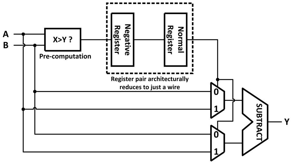
2.1. Architectural Retiming
Architectural Retiming gets its name because it both reschedules operations in time and modifies the structure of the circuit to preserve its functionality. It works by eliminating the latency introduced into a circuit by pipeline registers using the concept of a negative register (
Figure 1). A negative register is an architectural device that contains correct information before the completion of the logic itself. This can be implemented using pre-computation or prediction [
11]. With pre-computation, the negative register is synthesized as a function that pre-computes the input to the normal pipeline register using signals from previous pipeline stages. With prediction, the negative register's output is predicted one clock cycle before the arrival of its input using a finite state machine. When a negative register is paired with a normal register the result is architecturally just a wire and does not slow the critical path (assuming predictions are correct).
Architectural Retiming allows for a circuit to continue computation, rather than waiting for the end of a clock cycle, when the result of a pipeline stage finishes early. Pre-computation generates a bypass, an architectural transformation that increases the circuit performance, but it can only do so if there is enough information in the circuit to allow for pre-computing the value one cycle ahead of time. If the information is not available, the circuit can rely on an oracle to predict the value instead, these are usually synthesized with some sort of idea of what the logic will be doing and can be application specific. If a prediction is performed, it is necessary to verify the predicted value one cycle after the prediction when the actual value is computed. If the prediction is correct, the system can proceed with the next prediction. If the prediction was incorrect, the mis-predicted value must be flushed and the circuit should be restored to the previous state. This results in at least one cycle latency penalty. The applications of this technique are limited and the area and power overhead of the pre-computation or the prediction circuit is high.
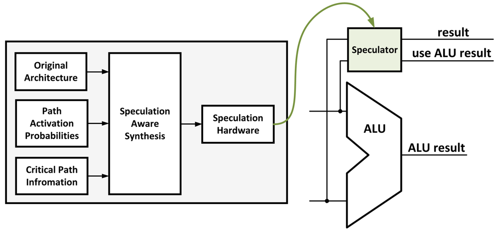
2.2. Circuit-Level Speculation
Circuit-Level Speculation [
12] is a method introduced to reduce the critical path of the circuit using approximation, implementing only a portion of a circuit. The approximated implementation of the circuit is the most heavily used part of the original circuit based on simulation results. A redundant full circuit is implemented and works in parallel to verify the approximated result in the next cycle (
Figure 2). Although this method results in a potentially large speed-up, it also requires a larger area and thus more power consumption. For example, when implementing a partial adder in the critical path, a complete adder has to work in parallel as well as an additional adder to compare the results in the next cycle. The energy overhead of this technique makes it infeasible for use in low-power applications. The circuit may also suffer a delay penalty if the approximated result does not match the complete result.
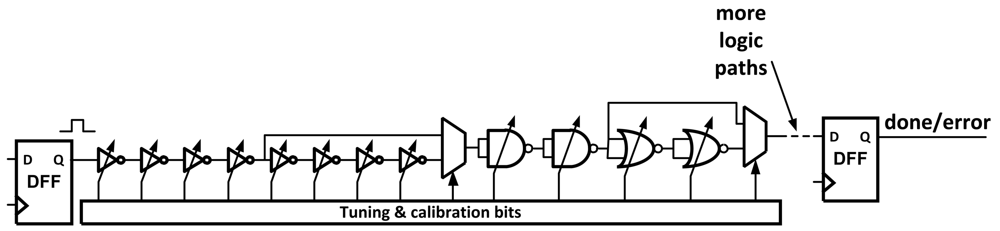
2.3. Tunable Replica Circuits
One method for finding errors due to voltage and frequency changes is the use of Tunable Replica Circuits (TRCs) [
9]. These circuits are composed of a number of digital cells, such as inverters, NAND, NOR, adders, and metal wires that are tunable to a given delay time (
Figure 3). The replicas are effected by process variations and aging in a similar way to the critical path. Once the replica is tuned to the critical path, it will replicate the path delay as it changes due to these variations. The TRCs can be used to report the critical path delay using a thermometer code or perform dynamic error detection.
TRCs are able to detect errors without introducing additional components or time delays to the data path. After being tuned once, the TRCs will mirror slightly worse than the critical delay path to ensure that any timing violation will be observed.
TRCs do suffer from a few drawbacks. Because the circuit is only a worst case replica, it is possible that they will trigger error responses when there was not a timing violation in the actual data path. The circuits themselves also take up area and power. Finally, TRCs cannot adapt to unique delay paths, only a simple worst case. This can make them hard to calibrate correctly under extreme variations as the TRC's timing margin needs to be large enough to guarantee all errors will be caught correctly.
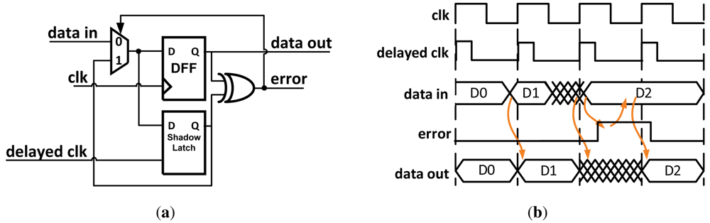
2.4. Razor Flip-Flops
Razor [
13] works by pairing each flip-flop within the data path with a shadow latch which is controlled by a delayed clock. As shown in
Figure 4, after the data propagates through the shadow latch the output of both of the blocks is XOR'd together. If the combinational logic meets the setup time of the flip-flop, the correct data is latched in both the data path flip-flop and the shadow latch and no error signal is set. Different values in the flip-flop and shadow latch indicates an erroneous result was propagated, and when an error is detected a logic-high signal is broadcast to an error recovery circuit as described in Section 3. The possibility exists that the datapath flip-flop could become metastable if setup or hold-time violations occur. Razor uses extra circuitry to determine if the flip-flop is metastable. If so, it is treated as an error and appropriately corrected.
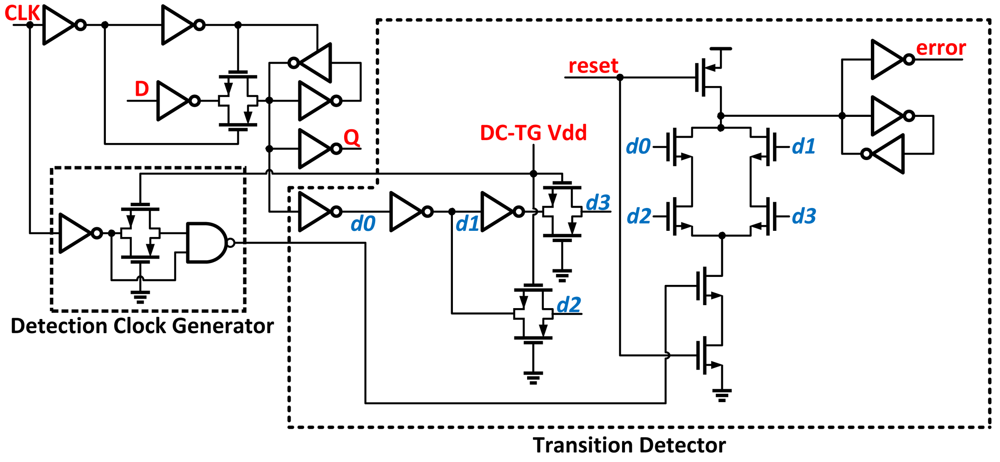
Razor II [
14] uses a positive level-sensitive latch combined with a transition detector to perform error detection
Figure 5. Errors are detected by monitoring transitions at the output of the latch during the high clock phase. If a data transition occurs during the high clock phase, the transition detector uses a series of inverters combined with transmission gates to generate a series of pulses that serve as the inputs to a dynamic OR gate. If the data arrives past the set-up time of the latch, the detection clock discharges the output node and an error is flagged. Replacing the datapath flip-flop from Razor with a level-sensitive latch eliminates the need for metastability detection circuitry. By removing the master-slave flip-flip and metastability detector, this version shows improved power and area over Razor.
When using Razor, it is important to be aware of the trade-offs that exist in achieving correct utilization of the timing window that enables Razor to properly detect errors. If a short path exists in the combinational logic and reaches the error latch before the delayed clock-edge of the computation preceding it, a false error signal could occur. To correct this, buffers are inserted in the fast paths to ensure that all paths can still be correctly caught. While this can help to guarantee a minimum timing constraint (hold time) of the shadow latch is met, it will also lead to additional area and power.
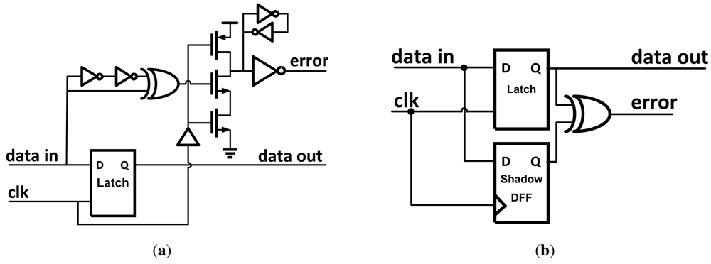
2.5. Transition Detectors
A number of other methods exist that also serve as capable error detection methods. The transition detector with time-borrowing (TDTB) [
4] is similar to Razor II in that it uses a dynamic gate to sense transitions at the output of a level-sensitive latch. Shown in
Figure 6(a), the TDTB differs from Razor II by using an XOR gate to generate the detection clock pulse, and the dynamic gate used in the transition detector uses fewer transistors.
Double sampling with time-borrowing (DSTB) [
4] is similar to the previous circuit but with the transition detection portion replaced with a shadow flip-flop [
Figure 6(b)]. Like Razor, the DSTB double samples the input data and compares the data path latch and shadow flip-flop to generate an error signal. The advantages of DSTB are that it also eliminates the metastability problem with Razor by having the flip-flop in the error path and retaining the time-borrowing feature from the transition detector. Clock energy overhead is lower than Razor since the data path latch is sized smaller than the flip-flop used in Razor. Aside from this, DSTB retains similar issues to Razor.
The static and dynamic stability checkers are introduced in [
15]. In the static stability checker, the data is again monitored during the high clock phase using a sequence of logic gates. If the input data transitions at all during the high clock phase, an error signal is generated. The dynamic stability checker uses a series of three inverters to discharge a dynamic node in the event of a data transition during the high clock phase, generating an error signal. In [
16] soft error tolerance is achieved by using a combination of time and hardware redundancy. This results in less hardware being used, but increases the time needed to check for errors.
3. Error Recovery Techniques
Once an error has been detected, a method needs to be in place to allow for the error to be dealt with properly. In a pipeline, later instructions may depend on the data generated by an earlier, errant instruction. Therefore these methods need to both assure the error is fixed (either by waiting enough time for the error to be corrected or re-executing the errant instruction) and make sure the erroneous instruction does not propagate the error.
Many pipeline error recovery techniques have been explored in the past. The most researched of these techniques are: Clock Gating [
2,
13], Counterflow Pipelining [
13], Micro-Rollback [
13], and Multiple Issue [
3]. The following section discusses each approach and their advantages and drawbacks.
3.1. Clock Gating
Clock Gating is conceptually the simplest technique to implement of all error recovery methods. Its original purpose was for saving power on unused blocks on a systems level by not clocking them when they are not used. This technique can also be adapted to error recovery by pausing all pipeline stages while waiting for the slow stage to either finish computation or to allow for the instruction to be re-executed. The pausing action ensures that later instructions do not continue to their next pipeline stage until the errant instruction is corrected. It is most commonly paired with Razor flip-flops as it only works if the pipeline can be stalled before the next clock edge, before the pipeline registers are set to get new data which can be achieved in slow systems. The Clock Gating concept is illustrated in
Figure 7.
The primary advantage to this method is that it requires very little architectural changes as well as minimal area addition to a design compared with other methods. However, in order for this method to work properly, a stall signal needs to propagate to all pipeline stages in a very short amount of time (50% of one clock cycle when Razor circuits are used). This can be difficult to achieve across large CMOS dies where pipeline stages are several millimeters apart. Furthermore, this is completely impractical to implement in complicated microprocessors because it may take several clock cycles just to propagate the clock signal through a clock distribution network which cannot be halted in only one cycle.
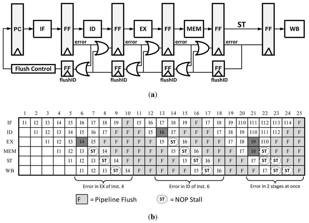
3.2. Counterflow Pipelining
Traditional Counterflow Pipelining is a microarchitecture technique that uses a bidirectional pipeline, allowing instructions to flow forward and results to flow backward. This technique made it easier to implement operand forward, register renaming, and most importantly pipeline flushing [
13,
17]. In order to modify this technique for error recovery, a traditional pipeline is modified such that only the flush signals are bi-directional. This concept is depicted in
Figure 8. In the event of an error, flush registers begin to propagate the error signal until it reaches the flush control unit. At that point the Program Counter (PC) is updated with a corrected instruction pointer and the pipeline continues operation. Because the flush registers clear the pipeline in both directions as the error is propagated, there is no need to do anything other than resume execution after the error has finished propagating. An illustration the Counterflow Pipeline instruction flow can be found in
Figure 8(b).
This method only requires local information to determine a stall, there is no global stall signal that needs to be computed and transmitted such as in clock gating. However, depending on how this method is implemented the area/power overhead can get quite large. For example, there need to be several PC values stored in the Flush control unit or in the flushID registers themselves; this overhead can get large in a 64-bit CPU with high pipeline depth. Unlike Clock Gating, this method takes several more cycles to recover from an error as the error propagates back one stage per cycle and the pipeline needs to be flushed.
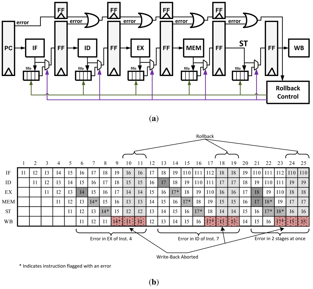
3.3. Micro-Rollback
Micro-Rollback is a technique that saves a queue of previous instructions and operands at each pipeline stage [
18]. After a successful operation, each stage saves the results as they are passed to the next stage. If an error is detected, instructions can be restarted at their last known correct state in the pipeline. Once an error is detected a signal is propagated with the instruction as it continues through the pipeline. Once the instruction reaches the write-back stage, rollback logic is activated to stop the instruction from being written and sends a signal to all of the pipeline stages to roll back and retry the instruction. The Micro-Rollback architecture is illustrated in
Figure 9(a). In its original design, instructions were simply replayed with the hope of the error being resolved at a later time. This is not very robust but with small architectural modifications this method can be redesigned to replay instructions twice or three times to ensure no error is produced a second time.
Using this technique makes the recovery process several cycles long. However, it reduces the error propagation/control overhead at each pipeline stage as required in the previous two techniques, leading to a faster clock speed. Unfortunately because of the addition of the queues, energy consumption may grow by 15% or more [
13].
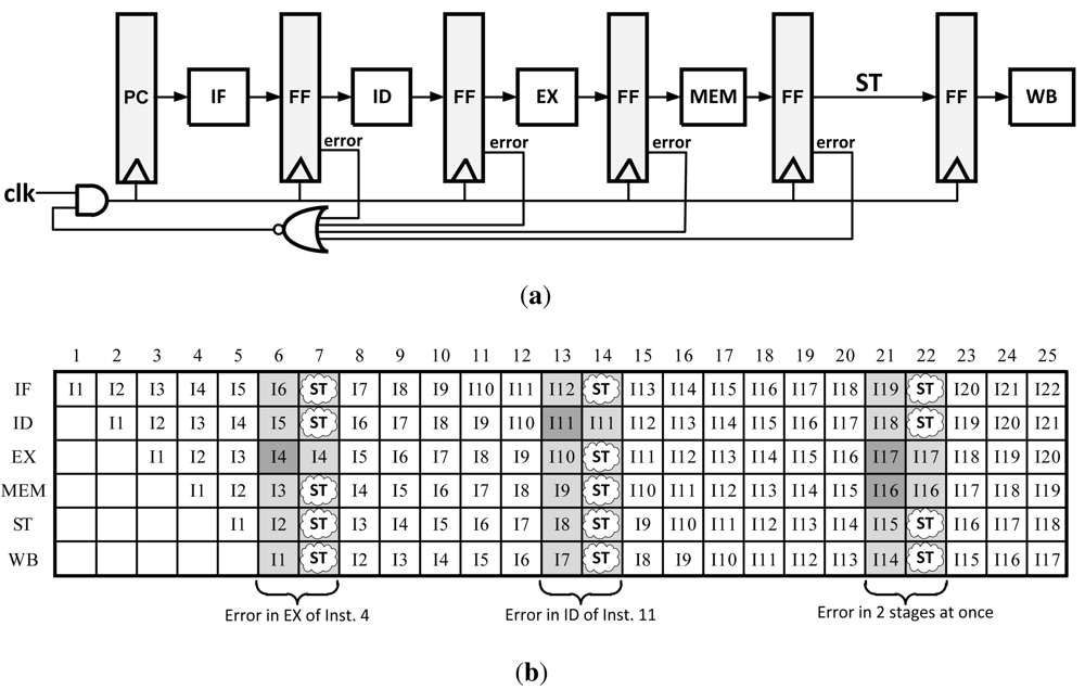
3.4. Multiple Issue
This method, shown in
Figure 10, has the simplest architecture of all the correction schemes. Similar to Micro-Rollback, errors propagate to the write-back stage, but instead of rolling back to a specific state, the entire pipeline is flushed and the erroneous instruction is replayed multiple times in succession to ensure completion of the previously failed operation. The amount of replayed instructions can vary depending on the expected delay of the erroneous stage. For example, in
Figure 10(b) the instruction is replayed three times. This is the most popular method proposed to be used in systems where corrected data cannot be captured after an execution cycle (such as in TRCs).
One advantage to this method is that it requires very small overhead in control logic, which results in less area and power. There is however a significant delay when a failed instruction is found, as the pipeline has to be flushed and the instruction replayed three times. Depending on the frequency of errors, this may result in a large average energy overhead per instruction as they take up many more clock cycles to complete. However, if these errors happen infrequently there is minimal penalty.
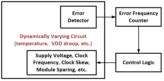
3.5. Adaptive Scaling Methods
Once an error (or errors) has been detected it may be beneficial to decrease the clock frequency or increase
Vdd to ensure that the frequency of errors decreases in the future. Adaptive scaling methods such as Dynamic Variation Monitors (DVM) [
19,
20] usually combine some type of error detector such as TRCs or RAZOR circuits with time-to-digital converters, error counters, or some type of prediction logic. If it has determined that errors are occurring too frequently, different circuit parameters such as
Vdd, core frequency, and clock skew are scaled accordingly. In the case of dynamic
Vdd droops this scaling can happen at a finer time-granularity. Courser tuning for slower changing variations such as instruction/data or temperature dependent delays can also be achieved.
Figure 11 illustrates this feedback process on the systems level.
3.6. Checkpoint-Restart
Checkpoint-restart (or checkpoint-rollback) is a common recovery technique. System state is occasionally preserved in a checkpoint. When an error is detected, state is rolled back to the most recent checkpoint and execution is restarted. Checkpoint-restart is traditionally a software technique, and its high overhead limits its applicability to very low error rates. Researchers proposed that the hardware structures of processors that support speculative execution can also be used for low-overhead checkpoint-restart [
21,
22]. Even with speculation hardware support, the overhead is still tens of cycles requiring a fairly low error rate to be effective.
3.7. Summary of Recovery Methods
Table 2 shows the advantages and disadvantages for each recovery method. It is clear that certain methods may prove to be better than others depending on the requirements of the pipeline and other system constraints. As far as complexity is concerned, it is clear that the Multiple Issue method performs the best, as Clock Gating is almost never practical in large systems. However, in a system where errors are more frequent and maximum clock speed is a concern, methods such as Counterflow Pipelining may be more beneficial.
4. Higher Level Error-Protection Techniques
Although this paper's main focus is on circuit level techniques, in this section we survey mechanisms in architecture and algorithm levels. Using these higher level approaches usually will not rely on error protection in levels beneath. Thus, it will allow achieving error protection while using commodity (non-protected) components. For example, architectural level techniques will provide error protection while using non-protected circuits, and algorithm level approaches can offer error protection while operating on commodity (non-protected) hardware.
Some if not all of the approaches described in this section have been initially designed in the context of system fault tolerance. As such, one of the basic assumptions of these approaches is fault randomness and independence. It makes these approaches suitable to handle random variation but limits their effectiveness in handling systematic variation.
4.1. Architecture Level Error-Protection Techniques
All architectural error protection approaches rely on some form of replication. Some techniques are using exact replication and therefore are more generic, while others provide error protection using simplified duplicated instances.
4.1.1. Dual Modular Redundancy
One of the simplest forms of architectural level error-protection is Dual Modular Redundancy (DMR). The protected module is replicated such that both the original module and its copy share their input signals [
Figure 12(a)]. Outputs are compared and a mismatch indicates an error. In case of an error, the system has to restore its last verified state and re-execute from that point. While having the advantage of design simplicity in using exact replication, this approach's disadvantages include high area and power/energy overheads. In addition it requires a roll-back and replay mechanism to recover in case of an error.
4.1.2. Triple Modular Redundancy
Triple Modular Redundancy (TMR) is similar to DMR, but this approach utilizes two replicated instances in addition to the original module [
Figure 12(b)]. The outputs of the three instances are compared and a majority voter mechanism is used to select the outcome signals. Based on the assumption that only one of the instances (at most) will fail at any given point, this approach eliminates the need for a roll-back and replay mechanism used in DMR, allowing instant recovery. One disadvantage is that it increases the area and power/energy overheads by adding the third instance of the module as well as increasing the critical path by adding the voter mechanism.
A generalized version of TMR is N-Modular Redundancy (NMR) also known as M of N redundancy. In this configuration, N instances of the module process the same inputs in parallel, and then use a majority voting scheme where M is the minimum number of modules required to get a majority count out of N modules. To summarize, NMR introduces xN power/area overhead and can tolerate at most N–M modules to fail.
4.1.3. Simplified Redundancy
To avoid the high overhead of the replicated module introduced in NMR schemes, it is possible to use a simplified version of the original module instead [
Figure 12(c)]. Several techniques based on this approach have been proposed. In [
23], the researchers propose using a simple (in-order) core as a checker for a complex control-intensive superscalar processor. The authors show that using a simple core as a checker significantly reduces the overheads compared to DMR while providing reasonable coverage.
A simplified checker approach can be used with arithmetic circuits as well. The key is to check the arithmetic operation with a similar operation of reduced bit-width. This is possible by transforming the operands into a reduced space with a transformation that is preserved under the arithmetical operations (+, −, ×, /). A common transformation used for this purpose is the residue code [
24]. The residue code works by transforming the operands, by calculating the remainder of their division by a constant A. Thus the outcome of the main arithmetic circuit can be verified by comparing its transformation (remainder of their division by a constant A in case of residue code) with the result of the checker circuit [
Figure 12(c)]. Although calculating a remainder can be a complicated operation, using 2
n − 1 as the constant A allows for calculating the reminder using simple logic and avoiding the expensive division. Using A = 3 will protect from all single bit flip errors, but might not detect some multiple bit flips. Error coverage can be increased using larger values of A.
Although the residue code is applicable to integer arithmetic only, there are some approaches to use it for floating point arithmetic by protecting various stages of floating point computations separately [
25]. In addition, other codes can be used in the context of floating point, like Berger codes [
26]. However, the disadvantage of the Berger codes is their lower coverage.
4.2. Architectural Data Protection
The same principles of redundancy can be applied in the context of data transport and storage structures. While it is possible to transport (or store) multiple copies of the same data to provide error protection, it is also possible to use a simplified (reduced) copy of the original data for protection purposes.
The simplest approach is known as a parity bit. By storing or transporting an additional bit whose value is equal to a XOR of all the bits of the data, a single bit flip error can be detected. This approach introduces very low overhead of a single additional bit. However, it can detect only a single bit flip and may not detect multiple bit errors.
While the parity bit approach provides a method for error detection only, the error-correcting codes (ECC) approach allows for the correction of the detected error, achieved by increasing the amount of redundant bits. Various approaches are available in the literature, varying the amount of error coverage and the overhead (
Table 3). The decoding and encoding logic for the simple codes shown in
Table 3 is negligible compared to the overhead of redundant storage and bandwidth [
27].
4.3. Software Level Error-Protection Techniques
Maintaining some level of error-protection while using non-protected hardware can be achieved using software level error-protection techniques. Being applied at the high level of software, these approaches are the most flexible in terms the trade-off between the error coverage and the overhead. However, these techniques are very limited in the amount of coverage they can provide.
4.3.1. Assertion Based Error-Protection
A very efficient way to detect errors in computation is to add assertions and invariant checks based on algorithmic knowledge [
33–
35]. This approach can be effective in some cases [
36], however, the error coverage that can be achieved in the general case is relatively low. In addition, assertions often require expert knowledge and utilize algorithm-specific traits, both of which are not always available.
4.3.2. Algorithmic Based Fault Tolerance (ABFT)
Using a modified version of the algorithm that operates on redundancy encoded data to verify the main result can be used for errors detection. In addition, in specific cases it can also allow error correction. This approach has relatively low overhead and potentially can provide high error coverage.
Various algorithms implementing ABFT are available in the literature [
37–
43]. However, the disadvantage is that this technique should be tailored specifically for each algorithm, requiring time-consuming algorithm development. Moreover, this approach is not applicable to an arbitrary program.
4.3.3. Arithmetic Codes
Perhaps the simplest example of an arithmetic code is the AN code [
24] (also known as linear residue code, product code, and residue-class code) applicable for addition (and subtraction) operations on integers. The operands are encoded by multiplying them by constant A. Based on the arithmetic properties of addition (subtraction), the result should also be a multiple of A. Thus, it allows validating the result, signaling error in case it is not a multiple of A.
4.3.4. Instruction Replication Techniques
Instruction replication, which introduces computational redundancy by duplicating all instructions in software, is arguably the most general software-level technique. While very general and amenable to automation [
44–
47], instruction replication has potentially high performance and energy overheads. Attempts have been made to minimize this overhead by executing instructions back-to-back in the same functional unit. This approach might be sufficient to detect particle-strike type errors but a different approach is necessary to detect variation-induced errors, such as executing at different times to detect voltage-variation related errors or on different functional units to address static variations.
5. Error Detection and Recovery in the Sub/Near-Threshold Regime
Sub-threshold operation differs from super-threshold mainly because the sub-threshold on-current depends exponentially on threshold voltage (
Vth) and
Vdd, while in super-threshold this dependence is linear [
48]. In [
48] it is shown that the variation of the on-current can be given by:
where
n is the sub-threshold swing factor (inversely proportional to
Vdd),
Vt is the thermal voltage, and standard deviation in the threshold voltage,
Vth, is proportional to
. This means there will be more variation in the sub-threshold on-current. Therefore, the delay in sub-threshold circuits will decrease dramatically first because of the exponential decrease in the speed of the transistors in this region, and second because of the added margins to the clock period due to exacerbated process variation.
When operating in the sub-threshold region, it is important to maximize operating speed while being aware of the increased delay variation (
Figure 13). Maximizing the speed will also help to limit the leakage energy of the circuit, making sub-threshold operation an even better alternative over super-threshold operation with respect to energy consumption. Unfortunately, few methods described in this review can properly operate in sub-threshold. The circuits themselves are also susceptible to increased process variation in sub-threshold, which can lead to unreliable operation. These slower speeds lead designers to push sub-threshold processors to a more parallel approach. For example, in [
8] the authors use multiple execution lanes to regain the throughput lost by the increased delays of sub-threshold operation.
The following subsections will discuss the viability of the techniques under review to operate in the sub-threshold region. We begin by discussing speculative error detection techniques and continue on with error recovery techniques. Finally, we will discuss specific techniques that have been designed for the purpose of sub-threshold operation.
5.1. Speculative Error Detection Techniques in Sub-Threshold
One of the biggest hurdles facing designers of sub-threshold error detectors is the uncertainty of the critical path. When designs are synthesized for super-threshold, accurate timing libraries are used to ensure the critical path is known and can be tested on-die. With the increased variations of sub-threshold the critical path may actually change as the voltage is lowered. This characteristic of sub-threshold operation makes speculative error detection techniques nearly impossible to operate efficiently.
First off, in order to use a speculative approach, a circuit must be well characterized. This would have to be done on a chip-by-chip basis as delays can change wildly from die-to-die. This process, just for a simple 32-bit multiplier, would take several decades. There may be some promise in using a reconfigurable speculative approach if a circuit could be accurately characterized on-die.
Non-speculative error-detection methods are the most promising for working in sub-threshold correctly. Methods like Telescopic units require that the critical path is well known and have the same issue as speculative techniques. However, more adaptive methods like TRC circuits have potential to operate correctly in sub-threshold. Moving sub-threshold circuits to a more asynchronous mode of operation probably is most promising for the variation tolerance needed in this region of operation. Razor circuits, if designed properly, can operate in sub-threshold. Section 5.3 discusses an implementation of a sub-threshold Razor system.
5.2. Error Recovery Techniques in Sub-Threshold
One of the most important factors to use when comparing any technique for sub-threshold operation is the energy overhead required to use it, especially the use of flip-flops as they consume an ill-proportionate amount of energy in sub-threshold. When comparing error-detection methods, there are two options that have minimal energy overheads. The most practical option is Multiple Issue as it has the lowest energy overhead while being a realistic option for robust error recovery. However, just as this method has a small energy/cycle overhead, it takes many more cycles to complete the recovery process. Depending on the frequency of errors this method may be completely impractical as the whole pipeline is leaking for 2N + 2 clock cycles. In order to determine which error recovery method is truly the best for sub-threshold, two factors must be taken in to account. Static energy overhead versus recovery time should be the metric used. The designer should determine the percentage of errors they expect to tolerate before using this metric, as energy per throughput could change dramatically as the frequency of errors is changed.
5.3. Sub-Threshold Timing Error Detection
One idea that exists in [
49] is to re-design the Transition Detector with Time-Borrowing (TDTB) circuit [
4]. By carefully sizing the transistors, they limit the
Vthvariation and obtain the optimal drive strength ratio of NMOS to PMOS for low-
Vdd operation. They also add extra logic to ensure correct functionality and use high-voltage threshold (hvt) transistors to reduce leakage as flip-flops are one of the largest contributors to sub-threshold leakage. This paper also uses a good method of measuring the effectiveness of an error detection circuit by generating a graph showing the upper and lower frequency limits that errors can successfully be detected at each voltage. As research into sub-threshold error detection continues, this will be a good metric to compare error detection methods against each other.
6. Conclusions
Variations of all forms must be dealt with in all time-constrained digital systems today. This paper summarized techniques to improve both the variation tolerance of these circuits as well as their throughput. Speculative techniques make a best guess of circuit delay based on known timing to improve throughput and potentially postulate timing induced errors. Non-speculative techniques are used primarily to detect errors as they happen or to sense the completion of a circuit on the fly. Once errors have been detected properly, error recovery methods are used to either stall or rollback the pipeline to ensure incorrect instructions are computed correctly. Furthermore, high-level techniques were explored that can improve robustness without the need for robust circuits.
Robust error detection and recovery can be challenging especially when operating in the sub-threshold region. Many of the techniques summarized in this review have great potential for robust operation under extremely variable conditions. The most valuable techniques that we believe will continue to be used in highly variable conditions are: well-designed Razor Circuits and recovery methods similar to the Multiple Issue method, paired with higher-level techniques such as error-correcting codes.


