Multivariate Weibull Distribution for Wind Speed and Wind Power Behavior Assessment


Abstract
:1. Introduction
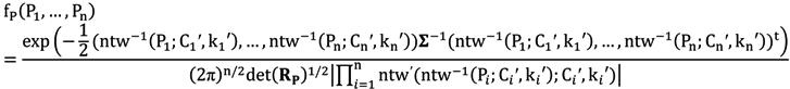
2. Multivariate Weibull Distribution
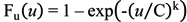
- (1)
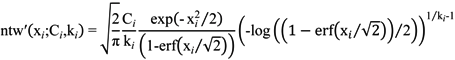
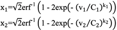
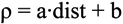
- The key point of the procedure is to define a change of variable from a Standard Normal to a Weibull distributed one. This transformation must be differentiable and the inverse function has to exist. The Standard Normal distributed variable is created in order to use its known features and transfer them to the Weibull one;
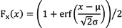
- (2)
- Establish as many changes as the number of variables, n, considering the different Weibull parameters for each case;
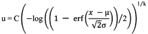
- (3)
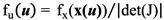
- Obtain the multivariate Weibull PDF from the multivariate Standard Normal PDF applying the change of variable.
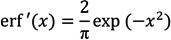
2.1. Normal to Weibull Change of Variables
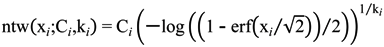


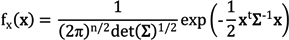
2.2. Multivariate Normal to Weibull Change


2.3. Multivariate Wind Speed Distribution
2.4. Multivariate Wind Power Distribution


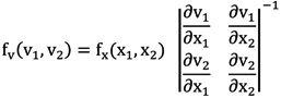
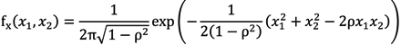
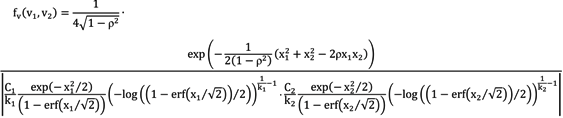
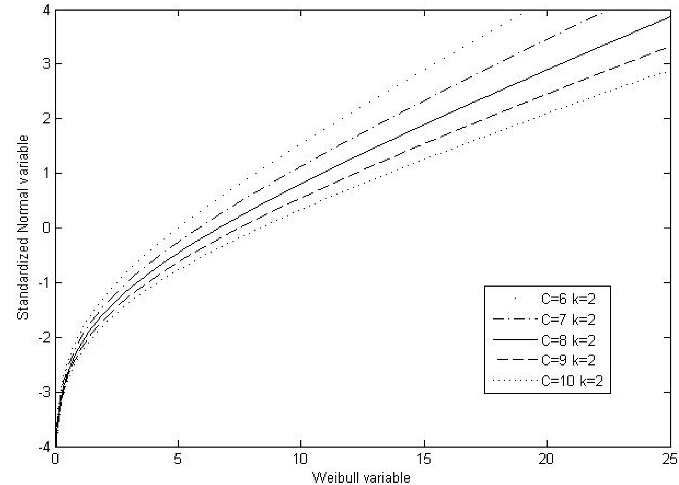
3. Bivariate Weibull Distribution
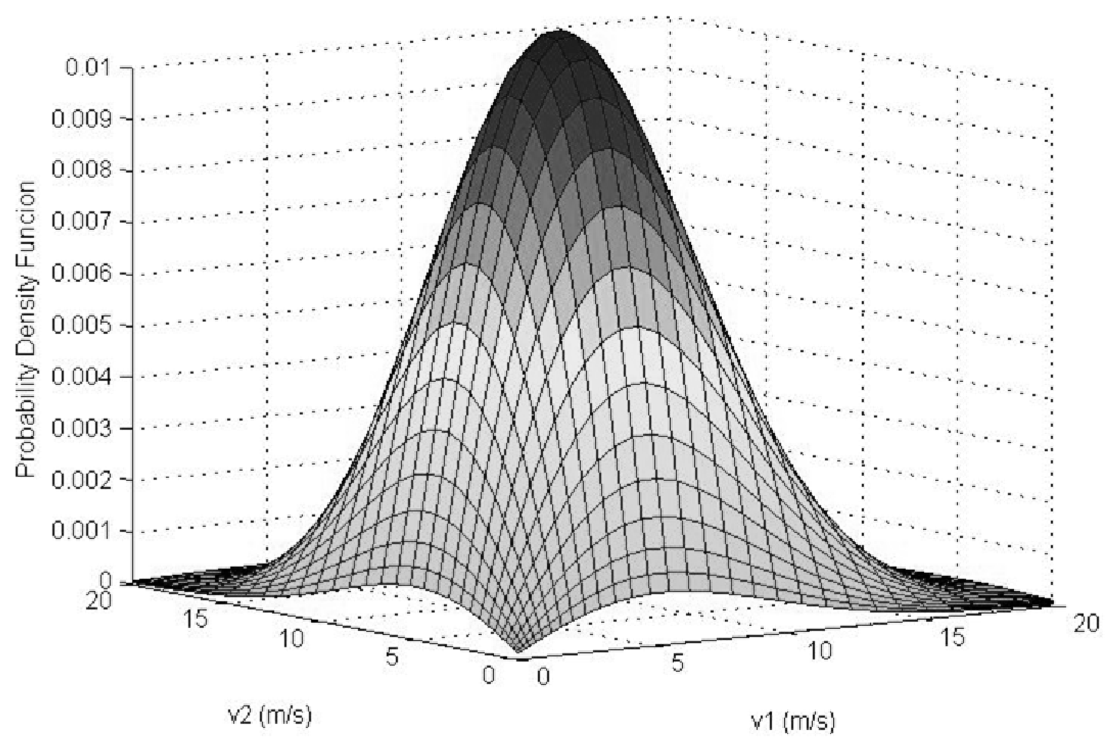
3.1. Bivariate Weibull Distribution Applied to Wind Speed

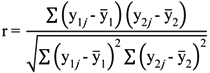
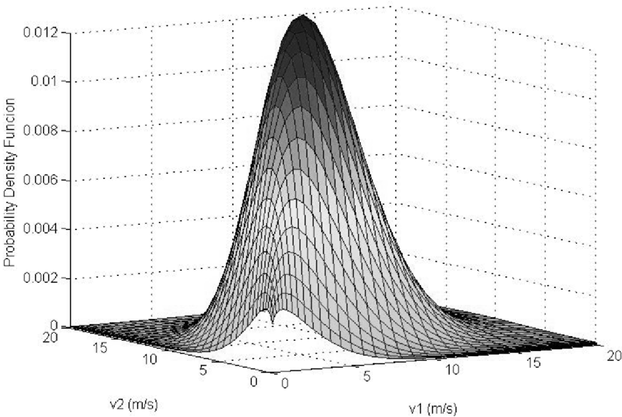
3.2. Correlation Coefficient Inference

H1:

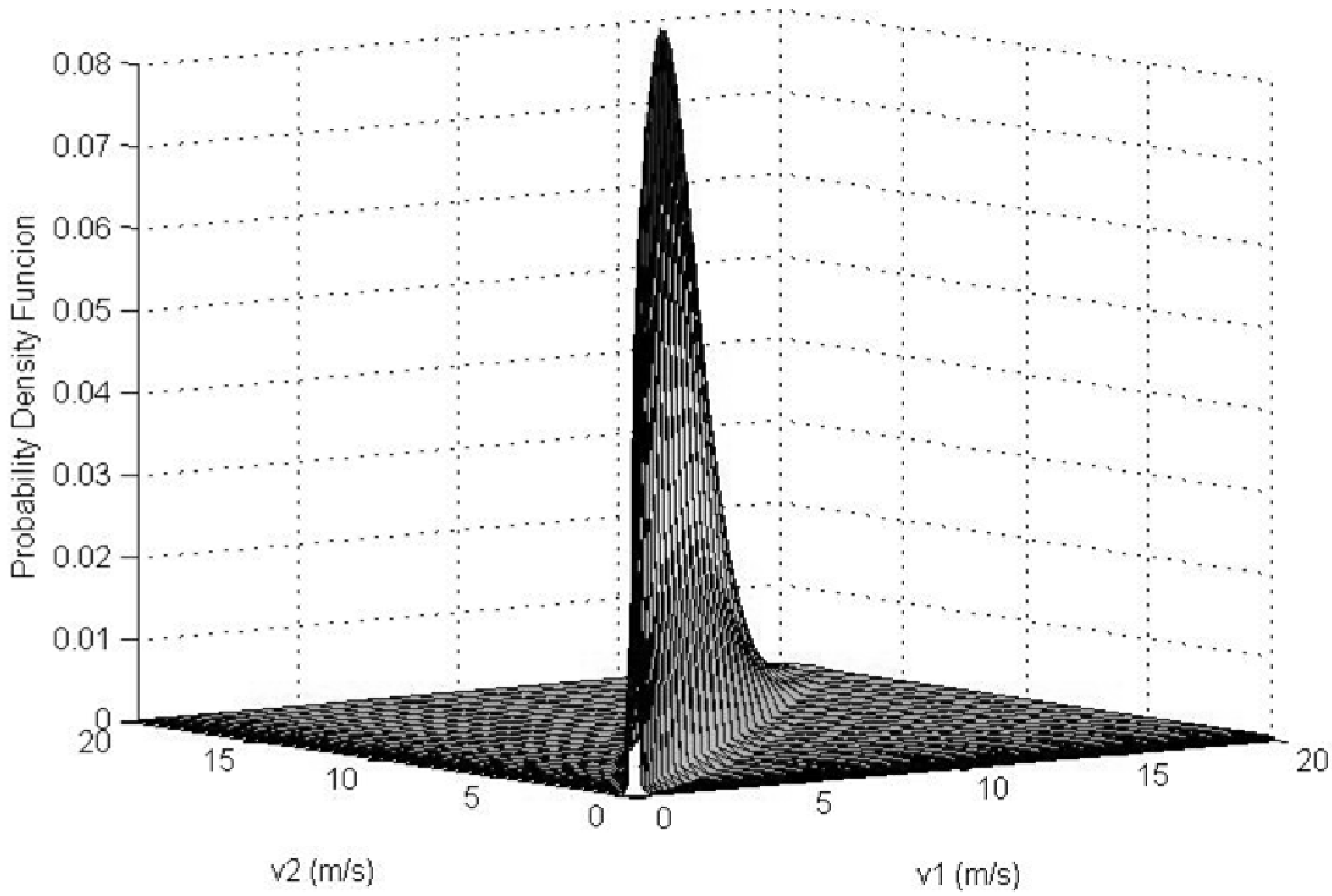
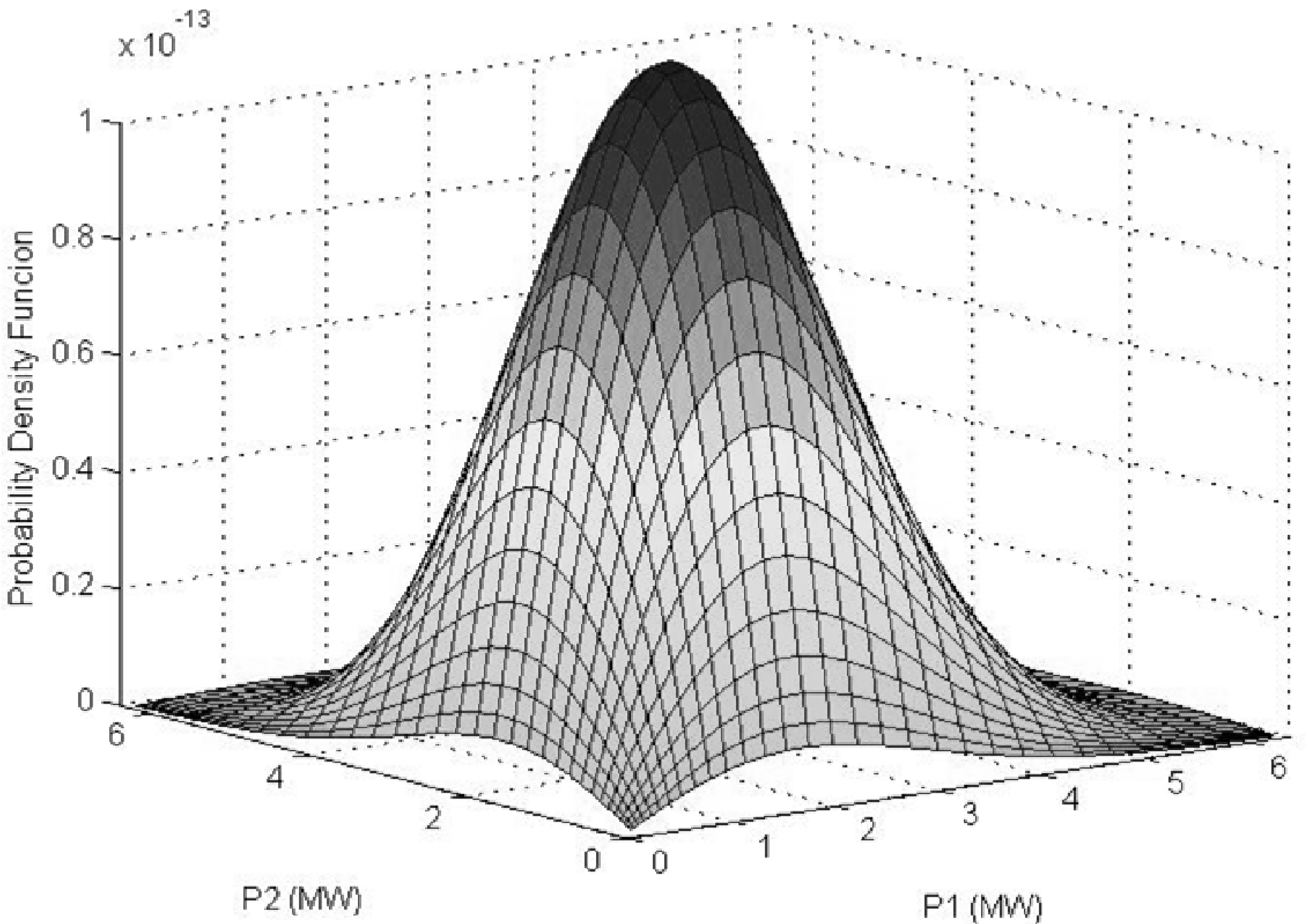
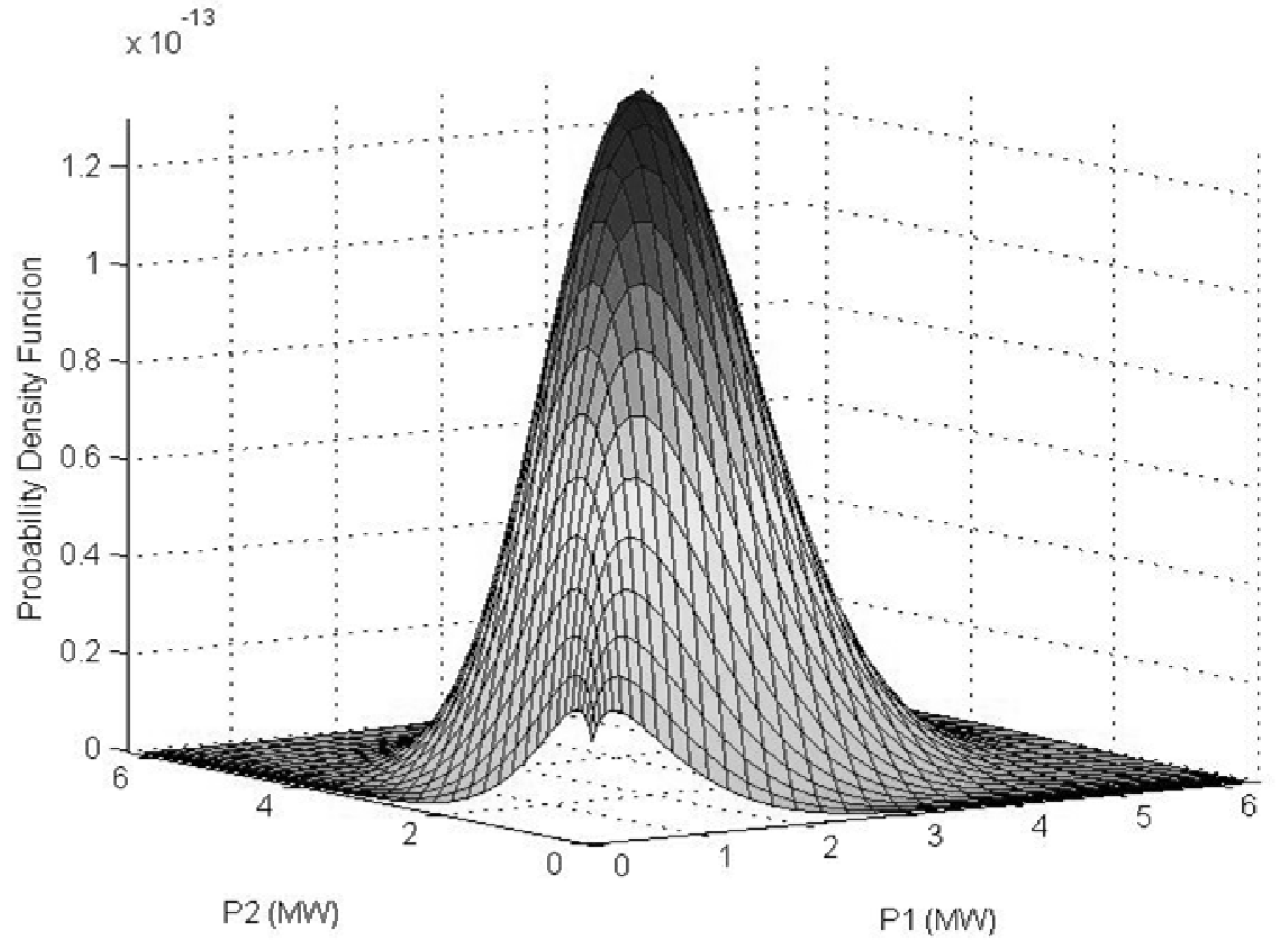
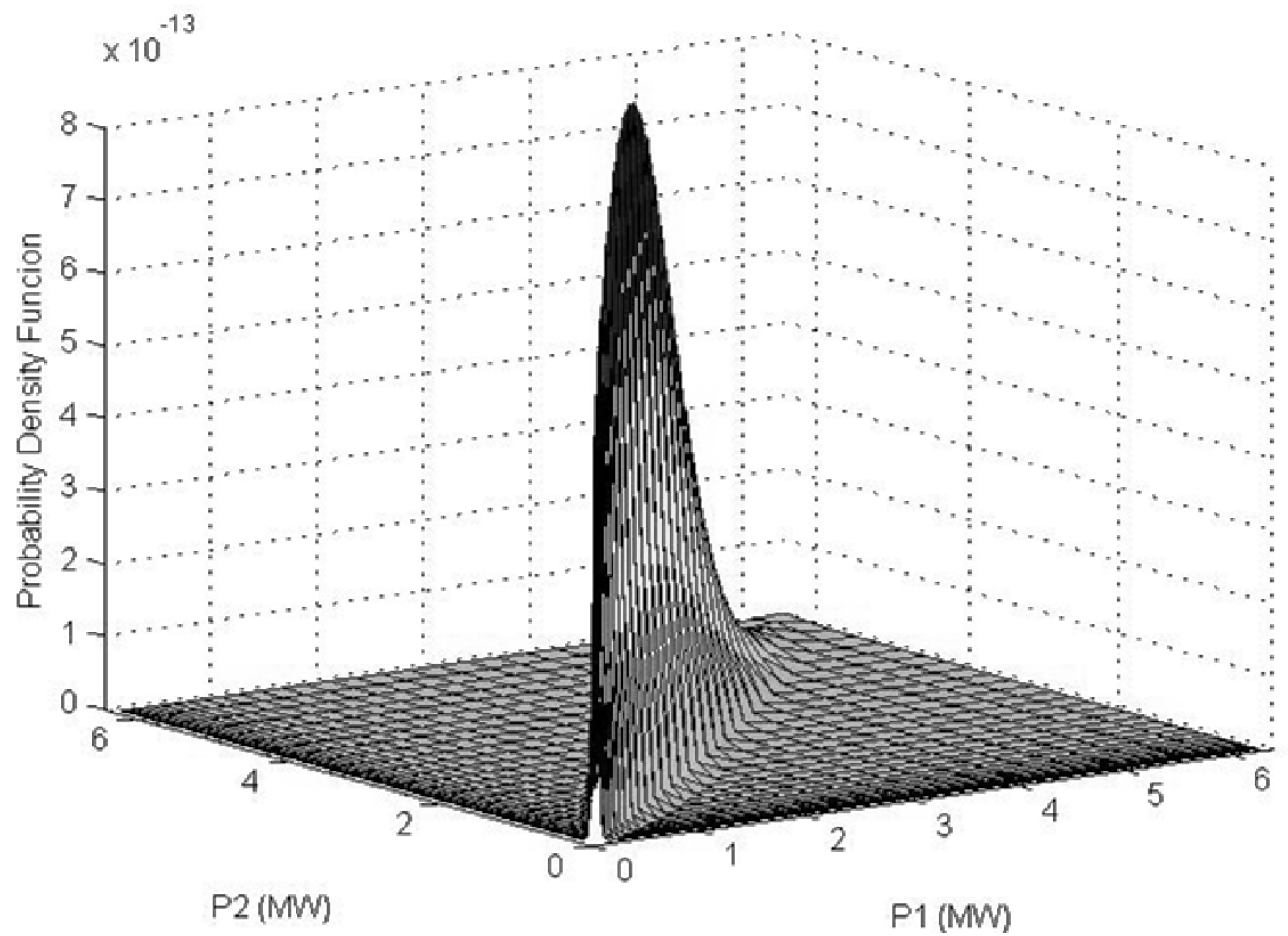
3.3. Bivariate Weibull Distribution Applied to Wind Power


4. Case Study


| Variable | Obtained value | Minimum value | Maximum value |
|---|---|---|---|
| r | 0.6202 | 0.5601 | 0.6394 |
| z | 0.7253 | 0.6330 | 0.7571 |
5. Conclusions
Appendix


 . Moreover, if µ1 = µ2 =…= µ and σ1 = σ2 =…= σ, then yji will follow a
  distribution. And, in the Standard case, if µ = 0 and σ = 1, then yji will be a
  distribution.
 , therefore in the particular case µ1 = µ2 =…= 0, σ1 = σ2=…= 1, yji will be distributed by a N(0,1) distribution.
Conflicts of Interest
References
- Weibull, W. A statistical distribution function of wide applicability. J. Appl. Mech. Trans. ASME 1951, 18((3)), 293–297. [Google Scholar]
- Devore, J.L. Probability and Statistics; Brooks/Cole: Belmont, CA, USA, 2010. [Google Scholar]
- Milton, J.S.; Arnold, J.C. Introduction to Probability and Statistics; McGraw-Hill: New York, NY, USA, 2002. [Google Scholar]
- Pham, H. Handbook of Engineering Statistics; Springer: Piscataway, NJ, USA, 2006. [Google Scholar]
- Murthy, D.N.P.; Xie, M.; Jiang, R. Weibull Models; John Wiley: Hoboken, NJ, USA, 2004. [Google Scholar]
- Marshall, A.W.; Olkin, I. A multivariate exponential distribution. J. Am. Stat. Assoc. 1967, 62, 30–44. [Google Scholar] [CrossRef]
- Lee, L. Multivariate distributions having Weibull properties. J. Multivar. Anal. 1979, 9((2)), 267–277. [Google Scholar] [CrossRef]
- Roy, D.; Mukherjee, S.P. Some characterizations of bivariate life distributions. J. Multivar. Anal. 1989, 28, 1–8. [Google Scholar]
- Crowder, M. A multivariate distribution with weibull connections. J. R. Statist. Soc. B 1989, 51((1)), 93–107. [Google Scholar]
- Lu, J.; Bhattacharyya, G.K. Some new constructions of bivariate Weibull models. Ann. Inst. Statist. Math. 1990, 42((3)), 543–559. [Google Scholar]
- Patra, K.; Dey, D.K. A multivariate mixture of Weibull distributions in reliability modeling. Stat. Probab. Letters 1999, 45, 225–235. [Google Scholar]
- Liu, P.L.; Kiureghian, A.D. Multivariate distribution models with prescribed marginals and covariances. Probab. Eng. Mech. 1986, 1((2)), 105–112. [Google Scholar]
- Morales, J.M.; Baringo, L.; Conejo, A.J.; Minguez, R. Probabilistic power flow with correlated wind sources. IET Gener. Transm. Distrib. 2010, 4, 641–651. [Google Scholar] [CrossRef]
- Troen, I.; Petersen, E.L. European Wind Atlas; Riso National Laboratory: Roskilde, Denmark, 1989. [Google Scholar]
- Wind turbines. Part 1: design requirements; IEC 61400-1; IEC Standards: Geneve, Switzerland, 2005.
- Freris, L.L. Wind Energy Conversion Systems; Prentice Hall: London, UK, 1990. [Google Scholar]
- Stuart, A.; Ord, K. Kendall’s Advanced Theory of Statistics; Oxford University Press Inc.: New York, NY, USA, 1994. [Google Scholar]
- Bronshtein, I.; Semendiaev, K. Handbook of Mathematics; Springer: New York, NY, USA, 2007. [Google Scholar]
- Lu, X.; McElroy, M.; Kiviluoma, J. Global potential for wind-generated electricity. Proc. Natl. Acad. Sci. USA 2009, 106, 10933–10938. [Google Scholar] [CrossRef]
- Correia, P.F.; Ferreira de Jesús, J.M. Simulation of correlated wind speed and power variates in wind parks. Electr. Power Syst. Res. 2010, 80((5)), 592–598. [Google Scholar] [CrossRef]
- Segura-Heras, I.; Escrivá-Escrivá, G.; Alcázar-Ortega, M. Wind farm electrical power production model for load flow analysis. Renew. Energy 2011, 36((3)), 1008–1013. [Google Scholar]
- Vallée, F.; Lobry, J.; Deblecker, O. System reliability assessment method for wind power integration. IEEE Trans. Power Syst. 2008, 23((3)), 1288–1297. [Google Scholar]
- Jobson, J.D. Applied Multivariate Data Analysis, Volume I: Regression and Experimental Design; Springer: New York, NY, USA, 1991. [Google Scholar]
- Johnson, R.A.; Wichern, D.W. Applied Mutivariate Statistical Analysis; Prentice Hall: Upper Saddle River, NJ, USA, 2007. [Google Scholar]
- Kleinbaum, D.G.; Kupper, L.L.; Muller, K.E.; Nizam, A. Applied Regression Analysis and Multivariable Methods; Thomson Brooks/Cole: Pacific Grove, CA, USA, 1998. [Google Scholar]
- Meteogalicia Homepage. Available online: http://www.meteogalicia.es (accessed on 1 November 2012).
- Freris, L.L.; Infield, D. Renewable Energy in Power Systems; John Wiley & Sons: Chichester, UK, 2008. [Google Scholar]
- Metropolis, N.; Ulam, S. The Monte Carlo Method. J. Am. Stat. Assoc. 1949, 44, 335–341. [Google Scholar] [CrossRef]
- Rubinstein, R.Y. Simulation and the Monte Carlo Method; Wiley Interscience: Hoboken, NJ, USA, 2008. [Google Scholar]
- Gentle, J.E. Random Number Generation and Monte Carlo Methods; Springer: New York, NY, USA, 2005. [Google Scholar]
© 2013 by the authors; licensee MDPI, Basel, Switzerland. This article is an open access article distributed under the terms and conditions of the Creative Commons Attribution license (http://creativecommons.org/licenses/by/3.0/).
Share and Cite
Villanueva, D.; Feijóo, A.; Pazos, J.L. Multivariate Weibull Distribution for Wind Speed and Wind Power Behavior Assessment. Resources 2013, 2, 370-384. https://doi.org/10.3390/resources2030370
Villanueva D, Feijóo A, Pazos JL. Multivariate Weibull Distribution for Wind Speed and Wind Power Behavior Assessment. Resources. 2013; 2(3):370-384. https://doi.org/10.3390/resources2030370
Chicago/Turabian StyleVillanueva, Daniel, Andrés Feijóo, and José L. Pazos. 2013. "Multivariate Weibull Distribution for Wind Speed and Wind Power Behavior Assessment" Resources 2, no. 3: 370-384. https://doi.org/10.3390/resources2030370