An Introduction to Environmentally-Extended Input-Output Analysis

Energy and Resources Group, University of California, Berkeley, 310 Barrows Hall, Berkeley, CA 94720-3050, USA
Resources 2013, 2(4), 489-503; https://doi.org/10.3390/resources2040489
Submission received: 10 July 2013
/
Revised: 24 August 2013
/
Accepted: 17 September 2013
/
Published: 30 September 2013
Abstract
:Environmentally-extended input-output (EEIO) analysis provides a simple and robust method for evaluating the linkages between economic consumption activities and environmental impacts, including the harvest and degradation of natural resources. EEIO is now widely used to evaluate the upstream, consumption-based drivers of downstream environmental impacts and to evaluate the environmental impacts embodied in goods and services that are traded between nations. While the mathematics of input-output analysis are not complex, straightforward explanations of this approach for those without mathematical backgrounds remain difficult to find. This manuscript provides a conceptual and intuitive introduction to the goals of EEIO, the principles and mathematics behind EEIO analysis and the strengths and limitations of the EEIO approach. The wider adoption of EEIO approaches will help researchers and policy makers to better measure, and potentially decrease, the ultimate drivers of environmental degradation.
Keywords:
input-output; environment; ecology; economics; biodiversity; indicator; consumption; sector1. Introduction
As human impacts on the natural environment continue to grow, methods that can identify the ultimate, upstream causes of these impacts are becoming increasingly important. Environmentally-extended input-output analysis (EEIO) is a long-established technique that continues to grow in popularity as a method for evaluating the relationship between economic activities and downstream environmental impacts. Among other applications, EEIO-based approaches have been recently used for analysis of the global carbon [1,2,3,4,5], water [6,7], ecological [8,9,10], nitrogen [11] and biodiversity/wildlife footprints [12,13]. This technique can be used to identify the economic drivers of any environmental impact, including the emission of pollutants, the degradation or harvest of natural resources and the loss of biodiversity.
While the basic mathematics of EEIO are not complex, simple, intuitive explanations of this technique for those without mathematical backgrounds remain difficult to find. This manuscript reviews the goals of EEIO, the principles and mathematics behind basic EEIO analysis and the strengths and limitations of the EEIO approach.
Readers who are interested in additional information on EEIO are encouraged to begin by consulting the comprehensive textbooks by Miller and Blair [14] and ten Raa [15], as well as the Eurostat Manual of Supply, Use, and Input-Output Tables [16]. Information on the development of new, global-scale input-output databases that are useful for EEIO applications can be found in several reviews [17,18] and in a recent special issue of the journal, Economic Systems Research ([19] and associated papers).
2. The Goals of EEIO
In the environmental literature, EEIO is generally used to accomplish one or both of two major goals:
- To calculate the hidden, upstream, indirect or embodied (these words are often used interchangeably) environmental impacts associated with a downstream consumption activity, such as the total carbon emissions that occur when a person purchases and consumes a hamburger;
- To calculate the amount of embodied environmental impact in goods traded between nations, such as how much nitrogen is released into the environment in the United States and then “exported” in wheat that is shipped to Denmark.
Traditionally, analysis of upstream environmental impacts and embodied impacts in traded products has been completed using process-based lifecycle analysis focused on individual products and a chosen upstream environmental impact. These traditional methods have several limitations, described below, that are addressed by EEIO approaches. EEIO approaches have other, different limitations, however, that are described in the Discussion section.
Throughout the examples below, the term “upstream” should be understood to refer to impacts associated with the various activities of sectors and industries that produce products that are eventually sold to end consumers. In some cases, there may be substantial impacts that occur directly at the level of the end consumer. For example, the carbon dioxide emission associated with the production of steel used to build a car would be an upstream impact, while the direct emission of carbon dioxide by a consumer who burns gasoline would be be a “zeroth layer” or direct impact. These direct impacts do not require the analysis described below and should instead be inventoried and assigned to the responsible consumers separately from the EEIO analysis.
All of the examples and analysis below employ a “consumer responsibility” philosophy, in which ultimate responsibility for environmental impacts is assigned to the end consumer who purchases a good or service [20]. This approach is the most common in the EEIO literature.
2.1. Total Impact Assessment of a Consumption Activity
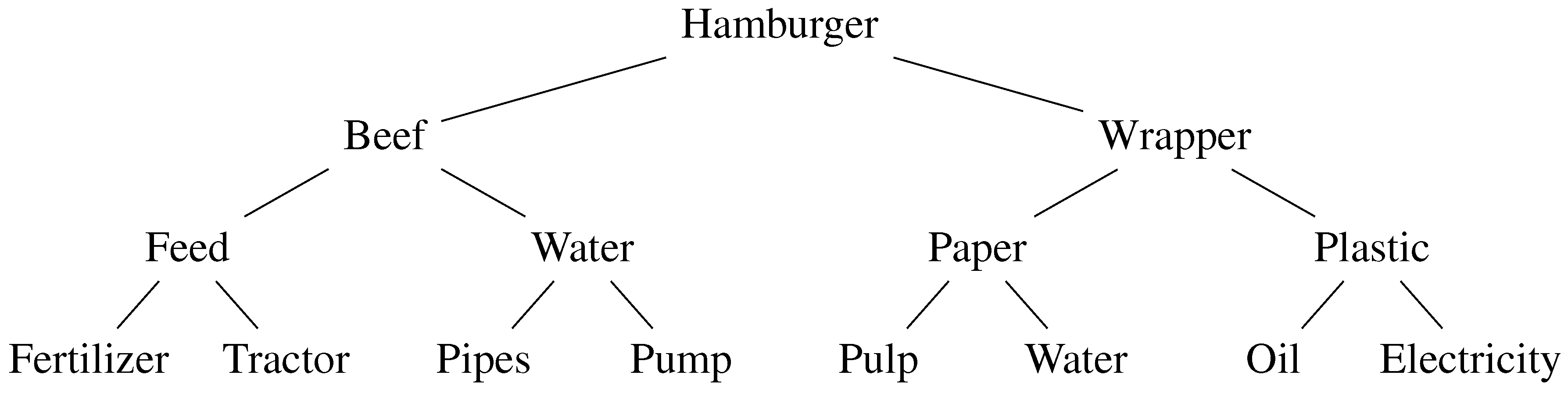
Consider, as an example, a consumer in the United States who purchases a hamburger and would like to know the total, upstream carbon emissions (or any other type of upstream environmental impact) that result from the production and sale of that hamburger. Following the hamburger backwards through the production process might result in a tree like that in Figure 1.
Figure 1.
Sample “production tree” showing upstream inputs required to provide a hamburger to a final consumer.
Figure 1.
Sample “production tree” showing upstream inputs required to provide a hamburger to a final consumer.

The creation of each of the products upstream from the hamburger (for example, the pipes used to transport the water, the fertilizer applied to the feed crop, etc.) requires an associated carbon emission. In principle, by adding up the carbon emissions associated with each upstream product, the total carbon emissions associated with the hamburger can be calculated. In practice, however, this approach has several limitations.
- This tree, in theory, continues back for an infinite number of production layers, but the number of upstream products that can be enumerated and analyzed is limited. If the analysis stops after only the first or second level, the estimate of the total emissions will suffer from truncation error and will almost certainly be an underestimate [21];
- Businesses may not make information about their production recipes publicly available, and it may thus be impossible to determine what particular inputs are used to produce an upstream product (for example, the hamburger wrapper) using this method;
- There may be cycles, or loops, in the tree. For example, the generation of electricity on the bottom right of the tree may itself require water, which requires pipes, which requires electricity again, and so on;
- Issues of double counting may arise. For example, some of the water used in the production of the paper may be recycled and used for watering crops afterwards. How should the carbon emissions associated with the transport and pumping of this water be divided between the paper and the crops? What if some of the pulp is made from recycled paper?
2.2. Embodied Impacts in Trade
In a similar fashion, consider, as an example, wheat that is grown in the United States and exported to other nations. Growing wheat involves the runoff of nitrogen within the US, and the question arises of how much that “virtual nitrogen” is exported from the US (or, equivalently, which nation’s consumers ultimately drive the runoff of nitrogen within the United States by eating finished products, such as bread). A similar tree (Figure 2) can be used to evaluate the flow of embodied environmental impacts in goods traded between nations.
Figure 2.
Sample diagram of trade flows of a product, wheat and two derived secondary products, bread and meat, between nations.
Figure 2.
Sample diagram of trade flows of a product, wheat and two derived secondary products, bread and meat, between nations.

This analysis has often been completed using a product coefficient approach ([22,23] and the discussion and references therein) that relies on product flow data from sources such as the Food and Agriculture Organization FAOSTAT database [24] or the United Nations Commodity Trade Statistics Database (COMTRADE) [25]. Because of the nation-of-origin tracking used in these databases, this approach is able to accurately measure imports and exports of raw products between nations (the link from the United States to Denmark in this example). However, several additional complications make these coefficient-based analyses difficult and potentially inaccurate.
- Trade statistics do not include information on second-step (or beyond) trade in processed products. For example, although FAOSTAT may correctly report the tonnage of wheat exported from the United States to Denmark, this does not necessarily mean that this amount of US wheat was eventually consumed in Denmark. If the wheat is processed into bread and exported to Germany, the “responsibility” for the associated environmental impacts of wheat production in the US should be allocated to German, not Danish, consumers. While data on exports of bread from Denmark to Germany are available, FAOSTAT and COMTRADE do not directly report the relationship between US wheat and bread consumed in Germany;
- Using identical logic to the above, products that are used as animal feed cannot be easily tracked by traditional coefficient-based analyses (livestock meat can be considered a secondary product, like bread, in this case);
- Traditional product-based approaches do not account for trade in services between nations. Consider, for example, the case of paper instead of wheat. If paper is used in a call center in India that exists to service the demands of US consumers, the upstream impacts of the production of this paper should arguably be allocated to US consumers, without whom the call center would not exist. This trade in services cannot be captured by traditional, product-based physical analyses;
- One-by-one evaluation of the flows of embodied environmental impacts embodied in several hundred or thousand products traded between several hundred nations rapidly becomes prohibitive.
3. Concept and Mathematics of EEIO
The basic concept of EEIO is to replace the manually-constructed trees of the previous section with a input-output matrix that shows flows, usually monetary, but sometimes physical, between economic sectors. In principle, for example, by measuring the amount of money that the beef sector spends in the feed (or agriculture) sector and measuring the carbon emissions per dollar of product sold by the feed sector, the amount of carbon emissions in the agriculture sector that are ultimately driven by the production of beef can be estimated. More generally, this approach can track flows of embodied impacts in products and services between many sectors of the economy simultaneously. By tracking the dollar value of German purchases of bread from Denmark and Danish purchases of wheat from the United States, the flows of these embodied impacts between nations can also be tracked.
The example below describes an open model, where the demand for goods and services by final consumers (such as households) is exogenous and separate from the activities of the production sectors, in which any and all products produced by the economy are consumed within the same economic system (i.e., there are no imports or exports). This is the most common approach used in global-scale EEIO analysis. For alternative model formulations, see Miller and Blair [14].
3.1. Definitions
Consider a world in which there are two economic sectors, agriculture (Ag) and manufacturing (Ma). These two sectors sell goods and services to each other and also to a population of final consumers who purchase the final, finished products sold by each of the sectors. This world can be described using the input-output table shown in Table 1.

Table 1.
Input-output table for two-sector world containing agriculture (Ag) and manufacturing (Ma) sectors. Other columns and rows give final demand (FD), value added (VA), total output (TO) and total input (TI).
| Ag | Ma | FD | TO | |
|---|---|---|---|---|
| Ag | 8 | 5 | 3 | 16 |
| Ma | 4 | 2 | 6 | 12 |
| VA | 4 | 5 | ||
| TI | 16 | 12 |
This table depicts all of the yearly monetary transactions between actors in the economy. The main square in the center of the table shows the inputs to each sector in the columns and the outputs, to each sector in the rows. In this example, businesses in the Ag sector purchase $4 worth of goods and services from the Ma sector and $8 worth of goods and services from other businesses in the Ag sector.
To the right of this central square are columns labeled FD, for final demand, and TO, for total output. FD gives the amount of money that final consumers spent to buy finished products from each sector. Although in most input-output tables, final demand consists of demands from households, government and businesses (gross fixed capital formation), this example considers only the summed final demand from these three sources, which will be referred to below simply as household demand. The total output of each sector is the total amount of goods and services sold, both to other businesses and to final consumers. The bottom square has rows for VA, or value added, and TI, for total inputs. Value added is the profit or economic benefit that sectors receive each year. Note that the total inputs into each sector equals the total outputs for that sector.
Next, imagine that the environmental impacts associated with all of the production activities of each sector in this year are known. For example, presume that an emissions inventory of this economy found that activities in the Ag sector resulted in the emission of 8 t of carbon, and activities in the manufacturing sector resulted in the emission of 4 t of carbon. The Ag sector, for example, may release 8 t C from soils in the process of generating all of its economic output for the year, while the manufacturing sector may burn 4 t C worth of fuel in its factories. Equivalently, an initial inventory showing that the Ag sector occupies 8 ha of land, and in the Ma sector, 4 ha could be used, as could a measure of any other quantifiable metric of environmental impact.
These emissions figures, along with knowledge of the total output of each sector, can be used to calculate a direct intensity vector, f, that gives the emissions associated with $1 of output from each sector. Ag has a direct intensity of 8 t C/$16 total output, or 0.5 t C/$. Ma has a direct intensity of 0.33 t C/$, and the direct intensity vector describes the emissions intensity for the two sectors in this economy.
If there were no intermediate sales between businesses in this economy and all products were purchased directly by final consumers, this would be the final step of the analysis. Ag products would have an intensity of 0.5 t C/$, and consumers would have had a final demand of $16 (the entire output of the Ag sector, since in this hypothetical case, consumers purchase the entire output of the sector), meaning that consumer purchases from the Ag sector drove the emission of 8 t C. Equivalent logic applies to the Ma sector. In terms of the input-output table, this would correspond to the case in which the entire main square of the table was filled with zeros.
However, because some of the products of each sector are sold to other businesses and not directly to final consumers, this simple calculation will not work here. A naive approach might be to multiply (elementwise) the direct intensity vector by a vector of actual final demand, , which results in a total emission estimate of , or only 3.5 t C worth of total emissions, with 1.5 t C from the Ag sector and 2 t C from the Ma sector.
Clearly, this approach is incorrect, as there are 8.5 t of “missing” carbon emissions. As explained below, these emissions are not missing at all—they are embodied in the intermediate products that businesses sold to each other. The value of EEIO lies precisely in its ability to capture the interrelationships between sectors in the economy and to sort out, in a simple and consistent manner, how these embodied emissions in intermediate products sold from business-to-business eventually become finished products and reach final consumers. EEIO thus provides a method for tracking how embodied impacts “move” from sector to sector, or nation to nation, in various forms of raw and finished products.
3.2. Mathematics: Preliminaries
The mathematics of EEIO are relatively simple, although basic matrix algebra is needed. The overall approach is explained graphically below, however, in an attempt to make the purpose and result of the matrix algebra more intuitive. To complete an EEIO analysis, two pieces of raw data are required: a measurement of the direct environmental impacts associated with each sector and a balanced input-output table in which the total inputs to each sector equal the total outputs from that sector. The example from the previous section is continued below, in which the measure of environmental impact is the emissions of carbon.
The first step, as previously described, is to divide (elementwise) the direct emissions for each sector by the total output for that sector to calculate a direct intensity vector, f, that gives the tonnes of carbon emitted by businesses in each sector to produce one dollar of output. In this vector, the first element refers to the first sector (Ag) and the second element to the second sector (Ma).
The second step is to create the technical coefficient matrix, commonly denoted as the A matrix [14], which gives the amount of input that a given sector must receive from every other sector in order to create one dollar of output. This matrix can be constructed by dividing each column in the central square of the input-output matrix, which gives the total dollar inputs into a sector, by the total output for that sector.
This matrix shows, for example, that the Ag sector requires $0.25 of inputs (that is, purchases) from the Ma sector for each dollar of output that it creates. This was found by taking the total inputs from the Ma sector into the Ag sector ($4) and dividing by the total output of the Ag sector ($16). All other cells of the A matrix are calculated in the same manner.
The next step is to consider how the flow of products between sectors and to final consumers can be tracked. Imagine that a consumer purchases a $1 shirt from a clothing business that is part of the Ma sector. What are the total upstream emissions associated with this shirt? This problem can be solved by successively moving upstream through layers of sales between sectors in this economy to find the total dollar output that was required from each sector, accounting for intermediate purchases between sectors, to create the shirt.
At the first layer, creating the shirt entailed $1 of direct output from the Ma sector, since this was how much the shirt cost. Thus, at a minimum, at least $1 of output from Ma is required. If the analysis was stopped at this first layer, this shirt would be estimated to require a carbon emission of 0.33 t C, which is simply the dollar output from the Ma sector ($1) multiplied by the direct intensity vector value for the Ma sector.
However, the input-output table (Table 1) shows that this shirt company had to purchase goods and services from other businesses in order to make the shirt. For example, it may have purchased cotton from a business in the Ag sector and plastic wrap from another business in the Ma sector. What was the total value of all of these purchases of inputs? Or equivalently, how much additional output “one layer behind” the shirt factory was required of each sector in the economy to support the production of the shirt?
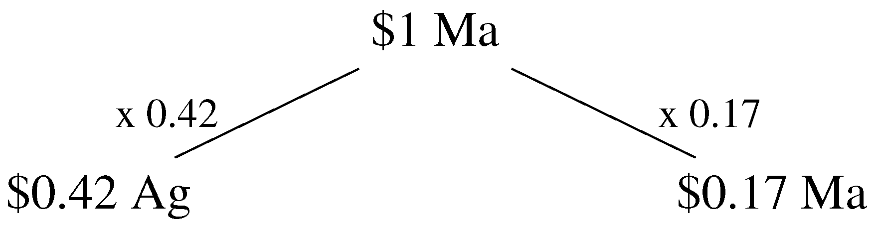
This question can be answered by examining the A matrix. The second column of the A matrix states that for a business in the Ma sector to create $1 of output, it must purchase as input $0.42 worth of goods and services from the Ag sector (the cotton business) and $0.17 worth of goods and services from the Ma sector (the plastic wrap business). Producing a $1 shirt thus required the additional output, at the second layer, of $0.42 from the Ag sector and $0.17 from the Ma sector (Figure 3).
Figure 3.
Sector output at production layers 1 and 2 required for the Ma sector to sell a $1 product to a final consumer.
Figure 3.
Sector output at production layers 1 and 2 required for the Ma sector to sell a $1 product to a final consumer.

The second layer emissions associated with the shirt can be calculated by multiplying these second layer output values by the appropriate direct intensity vector values, giving an additional t C of required emissions beyond the 0.33 t C of emissions associated with the first layer. The total estimate of the carbon emissions associated with this shirt are now t C, through the first and second layers of production.
This logic continues to the third layer, as the $0.17 of additional output from the Ma sector at layer two required more output from both the Ag and Ma sectors, once again in the proportions specified by the second column of the A matrix. Similarly, the $0.42 of output from the Ag sector at layer two requires additional output from the Ag and Ma sectors in the proportions specified by the first column of the A matrix, which gives the required inputs for one dollar of output from the Ag sector (Figure 4).
Figure 4.
Sector output at production layers 1, 2 and 3 required for the Ma sector to sell a $1 product to a final consumer.
Figure 4.
Sector output at production layers 1, 2 and 3 required for the Ma sector to sell a $1 product to a final consumer.
This third layer of production thus adds a total of dollars of required additional output from the Ag sector and dollars of required output from the Ma sector. As with the second layer, the total additional emissions required from this third layer of production can be calculated using these totals and the associated values from the direct intensity vector. The additional emissions from this third layer are t C, above and beyond those already counted in the first and second layers.
This process continues to an infinite number of upstream layers, although it should be clear that the contribution of successively higher (farther upstream) layers diminishes. In principle, the process above could be continued to calculate the carbon emissions associated with each layer of production. This would rapidly become infeasible, however, for large input-output tables, as the number of tree branches grows as the number of sectors to the power of the layer number. Fortunately, however, there is a faster way to perform this calculation, as explained in the next section.
3.3. Mathematics: Total Intensity Vector
Consider now how to calculate the total carbon emissions, from all layers of production, required to produce $1 of output from all sectors for sale to a final consumer (the same goal as the shirt example above). This new vector, giving the total carbon emissions associated with $1 of output to final demand, is known as the total intensity vector, F.
To begin, consider the first layer. At this layer, $1 of output to final demand involves just the directly emitted 0.5 t C for the Ag sector and 0.33 t C for the Ma sector. The total intensity vector, considering only the first layer, is thus the same as the direct intensity vector. In matrix form, the total intensity vector can thus be written as the product of the direct intensity vector and an identity matrix.
As with the direct intensity vector, the first element of this vector refers to the first sector (Ag) and the second element refers to the second sector (Ma).
Now, consider the second layer. For $1 of output to final demand from the Ma sector, for example, an additional $0.42 of output from the Ag sector (and 0.20 t C) and $0.17 of output from the Ma sector (and 0.06 t C) is required (see the previous section for explanation), for a total of 0.26 additional t C. Examining the A matrix, it becomes clear that this total can also easily be calculated by multiplying the direct intensity vector by the second column of the A matrix. In fact, this operation performs exactly the same steps of arithmetic as seen in the shirt example above, giving the same final answer. By the same logic, using the full A matrix, including the first column, also calculates the layer two emissions associated with $1 of output to final demand from the Ag sector, which are 0.33 t C.
Now, consider the third layer. The correct answer for the layer three output needed to produce $1 of output from the Ma sector is $0.28 from the Ag sector and $0.13 from the Ma sector. Although it may not be initially obvious, the equivalent algebra is carried out by squaring the A matrix, and these figures appear in the second column of the resulting matrix.
The second column of this squared matrix gives the dollar output from the Ag (first row) and Ma (second row) sectors required at the third layer, across all branches of the tree at this layer, to produce $1 of output to final demand from the Ma sector. Similar to the case of the second layer, this matrix can simply be multiplied by the direct intensity vector to find the layer three emissions associated with $1 of output from both sectors.
Similar to the previous production tree diagrams, this process can, in principle, be continued for higher layers. However, there is an additional manipulation that will allow the results for all layers to be calculated and summed in one step.
Examining the results for the first three layers, it can be seen that the total intensity vector across all layers, F, can be written as a sum of the intensity vectors for each layer, i, , and that each intensity vector is itself the product of f and either I (in the case of layer one) or A raised to a power.
The portion of this equation in brackets is a geometric series whose sum can be expressed as the function —that is, the infinite sum in the brackets is equal to this term. In reference to Wassily Leontief, who is considered to be the founder of input-output analysis [26], this new matrix is often known as the Leontief inverse matrix, L.
This is the equation most commonly used in applications of environmentally-extended input-output analysis. The actual matrix manipulation itself can be carried out in any numerical software package, including spreadsheet programs like Microsoft Excel, if the input-output matrices are relatively small.
Using the example data, F can be calculated to be equal to [1.6 1.2], which states that each dollar of output to final demand from the Ag sector requires 1.6 t of upstream carbon emissions (1.2 t C for the Ma sector).
3.4. Final Analyses
The total intensity vector, F, reports the total amount of upstream emissions (or other upstream environmental impact) that occur anywhere in the economy, in any sector, to ultimately produce $1 of output to final consumers from a given sector. In the case of carbon, this is often known as the emissions intensity of a sector. In terms of the earlier example, the upstream carbon emissions associated with the purchase of hamburger can be calculated by simply multiplying the price paid for the hamburger by the total intensity of the hamburger sector (or perhaps, more realistically, the bovine meat product sector).
The total upstream emissions caused each year by all of the sales to final consumers made by a sector can also be calculated. In the hamburger example, this would also be equivalent to the total emissions footprint of the hamburger sector or the total emissions that are ultimately driven by consumers purchasing and eating hamburgers. To do this, the total intensity vector (total emissions per dollar of final demand) is multiplied (elementwise) by the final demand vector (dollars of consumer purchases).
In the simple, two sector world, the emissions inventory counted total emissions of 12 t C, with 8 t C direct emissions from the Ag sector and 4 t C direct emissions from the Ma sector. However, after a more detailed analysis, consumer purchases from the Ag sector are found to be responsible for driving only 4.8 t C of upstream emissions, while purchases from the Ma sector are responsible for driving 7.2 t C of emissions.
The resulting vector E is sometimes referred to as a consumption-based inventory, as it counts all of the emissions required for a given sector to sell goods and services to end consumers. The original direct emissions inventory is then referred to as a production-based inventory.
Note that the total emissions from both sectors in the consumption-based and production-based inventories are the same (12 t C). This EEIO analysis can thus be interpreted as a process of reallocating responsibility for a known quantity of emissions (or impact, more generally) from a producer-orientation to a consumer-orientation. This result shows that there is effectively a net transfer of embodied carbon from the Ag to the Ma sectors in this economy. In other words, 3.2 t C emitted by the Ag sector are actually emitted to support the sales of goods and services from the Ma sector to final consumers. In theory, if the Ma sector did not exist, the Ag sector would only need to emit 4.8 t C in order to meet consumer demands for agricultural products.
Evaluating flows of embodied impacts between nations involves a very straightforward extension of the methods above. Imagine that there is a large input-output table in which there are, for example, 10 different nations, each with 25 different sectors, for a total of 250 sectors. Each sector in this large table can be identified by both a nation and a category, such as US manufacturing, US construction, Danish manufacturing, etc. The cells in this large input-output table now show not only the purchases between sectors within a nation, but also the purchases between sectors of different nations, a measure of import and export between nations. This table is known as a multi-regional input-output table [10,19].
In the multi-regional case, the F vector now gives the total upstream emissions from any sector in the world, not just sectors of the “home nation”, that are needed for a given sector within a given nation to sell its goods and services to end consumers. If the total intensity vector, F, is multiplied (elementwise) by a long vector of final demand of all of the households in Country A, , the result gives the total upstream impacts, in all nations, driven by the consumption of the residents of Country A. These summarized results can be disaggregated in many ways, including to measure bilateral trade between nations. When evaluated in this manner, the final emissions vector, , is often referred to as the total “footprint” of a nation, which represents the sum total of all upstream emissions required to produce all of the goods and services purchased by consumers in a nation from all sectors in a given year.
4. Discussion of Strengths and Weaknesses of EEIO Analysis
EEIO analysis provides a simple and rapid method that can be used to evaluate the upstream environmental impacts associated with downstream economic consumption, as well as the embodied environmental impacts in traded goods. This approach effectively addresses each of the major, previously described shortcomings of traditional process-based methods. In particular, EEIO is able to:
- Follow “product trees” back for an infinite number of steps;
- Use publicly available input-output tables to infer the production recipes used for the creation of goods and services;
- Address the existence of loops or cycles in production practices, which occur when a product is used in the production of itself;
- Avoid double counting by allocating, in a mutually exclusive manner, environmental impacts between sectors;
- Capture trade in secondary, processed products, including feed fed to livestock;
- Capture trade in services (if a monetary input-output table is used).
EEIO approaches also have several well-known limitations. Below are short descriptions of the most salient considerations for scientists who might apply EEIO techniques.
- Perhaps the most important assumption of EEIO is known as homogeneity, or the assumption that each sector in the economy products a single, homogeneous good or service. In other words, $1 sold by the Ag sector to every other sector and $1 sold by the Ag sector to final consumers is assumed to represent the same product or, at a minimum, carry an identical embodied environmental impact. This assumption becomes better as the resolution of the input-output table (i.e., the number of sectors) increases. Ideally, there should be one sector associated with each individual unique product created in the economy, although this level of detail is never realized;
- The sector resolution of input-output tables may be low, both leading to issues with homogeneity and with practical application. For example, the Global Trade and Analysis Project (GTAP) database, which is frequently used to create multi-regional input-output tables [27], has sectors for rice, wheat, and all other cereal grains. It is thus not possible, using this table, to specifically track the environmental impacts associated with soy beans, for example. It is similarly not possible to specifically track the impacts associated with a particular business within a sector using the simple methods described above;
- Input-output tables may not capture all activities in the economy. For example, they may exclude unpaid work and, as mentioned previously, will not generally include “zeroth layer” impacts, or direct impacts by consumers that do not involve purchases from economic sectors (i.e., burning gasoline in one’s car or cutting down and burning firewood on one’s own property). These issues may be especially important in low-income nations and for activities like land clearing, where much environmental impact may be “off the books”. The impacts of these activities should be inventoried and assigned directly to the relevant actors, without the use of input-output analysis;
- Input-output analyses are linear models that assume a constant, fixed proportion of inputs is used to create a sector’s output;
- The accuracy of global input-output tables is limited by disparities in the collection and standardization of raw data in different nations;
- Input-output tables are generally not available for every nation and may be published with large time lags (i.e., every five years);
- The accurate assessment of environmental impacts themselves, and the assignment of these impacts to sectors, is often difficult [28,29]. Inventories of environmental impacts, especially at large spatial scales, such as nations, often reflect a mix of empirically measured data and modeled estimates, both of which can introduce biases and uncertainties into EEIO analyses.
The extent and importance of these limitations will depend on the particular input-output database used for analysis. There are now several well-known multi-regional input-output databases and models that can be used for EEIO analysis at the global scale, including Eora [30,31], EXIOBASE [32,33], the Global Trade and Analysis Project (GTAP) [27,34,35], and the World Input-Output Database (WIOD) [36]. Newer databases have made a particular effort to address many of the limitations mentioned above, especially with regard to sector resolution.
5. Conclusions
Despite their limitations, applications of environmentally-extended input-output analysis continue to grow in popularity. By enabling the rapid assessment of the upstream drivers of environmental impacts, as well as the impacts embodied in trade between nations, this approach is enabling a new generation of analyses that take a consumption-focused, rather than a production-focused, perspective on the causes of global environmental degradation and resource use. This approach will be particularly critical for efforts to track the flow of resources and pollutants through an increasingly globalized economy and for finding ways to reduce the impacts of ever-growing human consumption demands. As newer and more detailed input-output tables continue to be created and as analysts move beyond traditional impacts, like carbon emissions, to evaluating impacts on water, land, resource use and biodiversity, environmentally-extended input-output analysis only stands to continue to gain in prominence and importance for years to come.
Acknowledgments
Support from the National Science Foundation (Graduate Research Fellowship Grant No. DGE 0946797) is gratefully acknowledged.
Conflicts of Interest
The author declares no conflict of interest.
References
- Peters, G.P.; Hertwich, E.G. CO2 embodied in international trade with implications for global climate policy. Environ. Sci. Technol. 2008, 42, 1401–1407. [Google Scholar] [CrossRef] [PubMed]
- Wiedmann, T. Editorial: Carbon footprint and input-output analysis—An introduction. Econ. Syst. Res. 2009, 21, 175–186. [Google Scholar] [CrossRef]
- Minx, J.; Wiedmann, T.; Wood, R.; Peters, G.; Lenzen, M.; Owen, A.; Scott, K.; Barrett, J.; Hubacek, K.; Baiocchi, G.; et al. Input-output analysis and carbon footprinting: An overview of applications. Econ. Syst. Res. 2009, 21, 187–216. [Google Scholar] [CrossRef]
- Davis, S.J.; Caldeira, K. Consumption-based accounting of CO2 emissions. Proc. Natl. Acad. Sci. USA 2010, 107, 5687–5692. [Google Scholar] [CrossRef] [PubMed]
- Davis, S.; Peters, G.; Caldeira, K. The supply chain of CO2 emissions. Proc. Natl. Acad. Sci. USA 2011, 108, 18554–18559. [Google Scholar] [CrossRef] [PubMed]
- Hoekstra, A.Y.; Chapagain, A.K. Water footprints of nations: Water use by people as a function of their consumption pattern. Water Resour. Manag. 2006, 21, 35–48. [Google Scholar] [CrossRef]
- Hoekstra, A.Y.; Mekonnen, M.M. The water footprint of humanity. Proc. Natl. Acad. Sci. USA 2012, 109, 3232–3237. [Google Scholar] [CrossRef] [PubMed]
- Bicknell, K.; Ball, R.J.; Cullen, R.; Bigsby, H.R. New methodology for the ecological footprint with an application to the New Zealand economy. Ecol. Econ. 1998, 27, 149–160. [Google Scholar] [CrossRef]
- Wiedmann, T.; Minx, J.; Barrett, J.; Wackernagel, M. Allocating ecological footprints to final consumption categories with input-output analysis. Ecol. Econ. 2006, 56, 28–48. [Google Scholar] [CrossRef]
- Galli, A.; Weinzettel, J.; Cranston, G.; Ercin, E. A Footprint Family extended MRIO model to support Europe’s transition to a One Planet Economy. Sci. Total Environ. 2013, 461–462, 813–818. [Google Scholar] [CrossRef] [PubMed]
- Leach, A.M.; Galloway, J.N.; Bleeker, A.; Erisman, J.W.; Kohn, R.; Kitzes, J. A nitrogen footprint model to help consumers understand their role in nitrogen losses to the environment. Environ. Dev. 2012, 1, 40–66. [Google Scholar] [CrossRef]
- Lenzen, M.; Moran, D.; Kanemoto, K.; Foran, B.; Lobefaro, L.; Geschke, A. International trade drives biodiversity threats in developing nations. Nature 2012, 486, 109–112. [Google Scholar] [CrossRef] [PubMed]
- Kitzes, J.A. Quantitative Ecology and the Conservation of Biodiversity: Species Richness, Abundance, and Extinction in Human-Altered Landscapes. Ph.D. Thesis, University of California, Berkeley, CA, USA, December 2012. [Google Scholar]
- Miller, R.; Blair, P. Input-Output Analysis: Foundations and Extensions, 2nd ed.; Cambridge University Press: Cambridge, UK, 2009; p. 750. [Google Scholar]
- Ten Raa, T. The Economics of Input-Output Analysis; Cambridge University Press: Cambridge, UK, 2005; p. 197. [Google Scholar]
- EUROSTAT. Eurostat Manual of Supply, Use and Input-Output Tables; Official Publications of the European Communities: Luxembourg, 2008. [Google Scholar]
- Wiedmann, T.; Lenzen, M.; Turner, K.; Barrett, J. Examining the global environmental impact of regional consumption activities—Part 2: Review of input-output models for the assessment of environmental impacts embodied in trade. Ecol. Econ. 2007, 61, 15–26. [Google Scholar] [CrossRef]
- Wiedmann, T.; Wilting, H.C.; Lenzen, M.; Lutter, S.; Palm, V. Quo Vadis MRIO? Methodological, data and institutional requirements for multi-region input-output analysis. Ecol. Econ. 2011, 70, 1937–1945. [Google Scholar] [CrossRef]
- Tukker, A.; Dietzenbacher, E. Global multiregional input-output frameworks: An introduction and outlook. Econ. Syst. Res. 2013, 25, 1–19. [Google Scholar] [CrossRef]
- Lenzen, M.; Murray, J.; Sack, F.; Wiedmann, T. Shared producer and consumer responsibility—Theory and practice. Ecol. Econ. 2007, 61, 27–42. [Google Scholar] [CrossRef]
- Lenzen, M. Errors in conventional and input-output-based life-cycle inventories. J. Ind. Ecol. 2000, 4, 127–148. [Google Scholar] [CrossRef]
- Moran, D.D.; Wackernagel, M.C.; Kitzes, J.A.; Heumann, B.W.; Phan, D.; Goldfinger, S.H. Trading spaces: Calculating embodied ecological footprints in international trade using a Product Land Use Matrix (PLUM). Ecol. Econ. 2009, 68, 1938–1951. [Google Scholar] [CrossRef]
- Tukker, A.; Koning, A.D.; Wood, R.; Moll, S.; Bouwmeester, M.C. Price corrected domestic technology assumption—A method to assess pollution embodied in trade using primary official statistics only. With a case on CO2 emissions embodied in imports to Europe. Environ. Sci. Technol. 2013, 47, 1775–1783. [Google Scholar] [CrossRef] [PubMed]
- Food and Agriculture Organization. Available online: http://faostat.fao.org/ (Accessed on 15 September 2013).
- United Nations Statistical Division. United Nations Commodity Trade Statistics Database. Available online: http://comtrade.un.org/ (accessed on 15 September 2013).
- Leontief, W. Quantitative input-output relations in the economic system of the United States. Rev. Econ. Stat. 1936, 18, 105–125. [Google Scholar] [CrossRef]
- Andrew, R.M.; Peters, G.P. A multi-region input-output table based on the global trade analysis project database (GTAP-MRIO). Econ. Syst. Res. 2013, 25, 99–121. [Google Scholar] [CrossRef]
- Jury, C.; Rugani, B.; Hild, P.; May, M.; Benetto, E. Analysis of complementary methodologies to assess the environmental impact of Luxembourg’s net consumption. Environ. Sci. Policy 2013, 27, 68–80. [Google Scholar] [CrossRef]
- Zhang, Y.; Singh, S.; Bakshi, B.R. Accounting for ecosystem services in life cycle assessment. Part I: A critical review. Environ. Sci. Technol. 2010, 44, 2232–2242. [Google Scholar] [CrossRef] [PubMed]
- Lenzen, M.; Kanemoto, K.; Moran, D.; Geschke, A. Mapping the structure of the world economy. Environ. Sci. Technol. 2012, 46, 8374–8381. [Google Scholar] [CrossRef] [PubMed]
- Lenzen, M.; Moran, D.; Kanemoto, K.; Geschke, A. Building EORA: A global multi-region inputoutput database at high country and sector resolution. Econ. Syst. Res. 2013, 25, 20–49. [Google Scholar] [CrossRef]
- Tukker, A.; Poliakov, E.; Heijungs, R.; Hawkins, T.; Neuwahl, F.; Rueda-Cantuche, J.M.; Giljum, S.; Moll, S.; Oosterhaven, J.; Bouwmeester, M. Towards a global multi-regional environmentally extended input-output database. Ecol. Econ. 2009, 68, 1928–1937. [Google Scholar] [CrossRef]
- Tukker, A.; de Koning, A.; Wood, R.; Hawkins, T.; Lutter, S.; Acosta, J.; Rueda Cantuche, J.M.; Bouwmeester, M.; Oosterhaven, J.; Drosdowski, T.; et al. EXIOPOL—Development and illustrative analyses of a detailed global MR EE SUT/IOT. Econ. Syst. Res. 2013, 25, 50–70. [Google Scholar] [CrossRef]
- Peters, G. From production-based to consumption-based national emission inventories. Ecol. Econ. 2008, 65, 13–23. [Google Scholar] [CrossRef]
- Peters, G.P.; Andrew, R.; Lennox, J. Constructing an environmentally-extended multi-regional inputoutput table using the GTAP database. Econ. Syst. Res. 2011, 23, 131–152. [Google Scholar]
- Dietzenbacher, E.; Los, B.; Stehrer, R.; Timmer, M.; de Vries, G. The construction of world input-output tables in the WIOD project. Econ. Syst. Res. 2013, 25, 71–98. [Google Scholar]
© 2013 by the authors; licensee MDPI, Basel, Switzerland. This article is an open access article distributed under the terms and conditions of the Creative Commons Attribution license (http://creativecommons.org/licenses/by/3.0/).
Share and Cite
MDPI and ACS Style
Kitzes, J. An Introduction to Environmentally-Extended Input-Output Analysis. Resources 2013, 2, 489-503. https://doi.org/10.3390/resources2040489
AMA Style
Kitzes J. An Introduction to Environmentally-Extended Input-Output Analysis. Resources. 2013; 2(4):489-503. https://doi.org/10.3390/resources2040489
Chicago/Turabian StyleKitzes, Justin. 2013. "An Introduction to Environmentally-Extended Input-Output Analysis" Resources 2, no. 4: 489-503. https://doi.org/10.3390/resources2040489